M4.1 - Transformer Cost Model: Parameters, Activations, FLOPs, and Memory Traffic

0x00 One Model Does Not Have One Cost

A neural-network description once fit comfortably into a short sentence: name the architecture, count its learned parameters, and report how many arithmetic operations one forward pass requires. Parameter count became a useful common language because it describes a stable property of the learned state. It does not depend on which GPU happens to load the checkpoint, and it gives a first approximation of how much capacity and weight storage the model carries.

That shorthand remains useful. It is not a cost model.

The same Transformer can appear in several technically correct statements:

the architecture contains this many learned scalars
the checkpoint occupies this many bytes on storage
one training rank owns this much persistent state
the forward/backward schedule reaches this live-memory peak
one prefill executes this much arithmetic
one decode step transfers this much persistent state
this runtime reaches this latency and throughput on this workload

Those statements do not measure the same object. None can replace all the others, and two of them can change in opposite directions. Sharding can reduce the persistent state owned by one rank while leaving the global learned state unchanged. Activation recomputation can lower the live-memory peak while adding arithmetic. Quantization can reduce representation bytes while introducing metadata, packing rules, and a different executable kernel contract. A fused kernel can reduce memory traffic without changing the mathematical operation count.

Transformer Series A16 - Resource Consumption introduced the right bottom-up instinct: begin with units and data types, then count parameters, memory, activations, operations, and bottlenecks. M4.1 keeps that staircase but makes each step conditional on an explicit execution contract. Modern models add grouped-query attention, gated MLPs, tied or untied vocabulary heads, mixed-precision state, sharded ownership, recomputation, persistent K/V state, fused operators, allocator reserve, and backend-dependent workspaces. The coefficient remembered from one policy can therefore be wrong even when its algebra was correct for the original policy.

0x00A From A Graph To An Executed System

M1.1 established the whole-model execution path:

token IDs
  -> embedding rows
    -> repeated Transformer blocks
      -> normalization and vocabulary projection
        -> logits and a next-token decision

M3.10 then showed that the graph is not executed with one universal shape:

training:
    process a declared batch and sequence distribution
    retain or reconstruct state required by backward
    update persistent optimization state

prefill:
    process the prompt rows
    create the request's initial K/V state
    produce logits under a declared output policy

decode:
    process a small query frontier
    read the retained prefix state
    append state for the next generation step

The architecture tells us which transformations exist. The workload tells us which tensor extents reach them. The numerical policy tells us how each state class is represented. The schedule tells us what must be alive at the same time. The parallel plan tells us which rank owns or temporarily materializes each object. The runtime tells us how logical work becomes physical transfers, kernel launches, synchronization, and elapsed time.

Cost accounting starts only after those layers are separated.

0x00B Why Correct Ledgers Can Disagree

Consider one declared decoder architecture. Its learned tensors can remain unchanged while its workload moves from training to prefill to decode. Its global state can remain unchanged while a parallel strategy changes per-rank ownership. Its mathematical graph can remain equivalent while a fused kernel changes intermediate materialization. Its output can remain within a declared quality contract while a quantized artifact changes the bytes and operations used to produce it.

The first discipline is therefore linguistic. Parameter count means the number of declared learned scalar entries. It is not automatically checkpoint size, device residency, training peak, operation count, traffic, latency, or energy. FLOPs describe an operation convention over an execution path. They do not say whether the hardware repeatedly fetched the same bytes or reused them on chip. Allocated tensor bytes do not automatically include allocator reserve, library workspaces, communication staging, or memory held outside the framework’s allocator.

A disagreement is informative when both sides publish their boundaries. It is misleading when one unlabeled number is allowed to stand for the whole system. For example:

global learned state != per-rank resident state
serialized bytes     != live device bytes
logical tensor bytes != measured memory transactions
analytic FLOPs        != achieved hardware operations
single-request time   != batched serving throughput
emitted output state  != every temporary branch state

This distinction is also why source-paper numbers cannot be transplanted by name alone. A scaling study may exclude one parameter class from its variable N; a systems paper may report model FLOPs utilization under another operation set; a memory paper may assume a particular optimizer, sequence-parallel plan, or recomputation schedule. M4.7 compares the empirical consequences of those study contracts. M4.1 first makes the accounting object visible.

0x00C Owner Question And Thesis

M4.1 owns the following question:

Given an immutable Transformer architecture, execution phase, numerical-state policy, parallel ownership plan, operation convention, and measurement boundary, which learned scalars, resident bytes, live tensors, arithmetic operations, communication payloads, and logical memory transfers does one declared workload require?

The article’s thesis is stricter than “count everything”:

A Transformer has no context-free cost. A useful cost model is a versioned accounting program. It starts from the executable graph and workload, derives several non-interchangeable ledgers, records the assumptions that produced each one, and reconciles predictions against an independently observed checkpoint, allocator, profiler, or run record.

The word program matters. A result should be reproducible from a manifest, not reconstructed from an unexplained multiplier. The following declaration is the method signature used by the rest of the article:

C = (
  graph and architecture manifest,
  workload and execution phase,
  numerical and persistent-state policy,
  liveness and parallel ownership,
  operation and transfer convention,
  observation and reconciliation boundary
)

0x00D The Six Accounting Contracts

Contract One: Graph And Architecture Manifest

The graph contract names the exact model family and revision being counted. It records the number of layers and residual width; query and K/V head counts; head dimension; MLP type and intermediate width; normalization layout; vocabulary size; embedding/head tying; bias policy; positional mechanism; and any experts, adapters, projectors, or other learned branches.

This contract prevents architectural folklore from replacing the executable object. “A Llama-like model” is not enough to determine whether the head is tied, whether biases exist, how K/V width is represented, or which extra state is stored. The model configuration and checkpoint schema are the source of truth. The next section turns this contract into the article’s running manifest.

Contract Two: Workload And Execution Phase

The workload contract declares whether the graph is used for training, evaluation, prefill, or decode. It records global and microbatch sizes, gradient accumulation, sequence lengths or their ragged distribution, cached length, active request count, mask policy, logits policy, and whether the boundary includes forward, backward, recomputation, and an optimizer step.

This is why “one forward pass” is still incomplete. A full-row training forward, a prompt prefill, and one-row decode can invoke the same weights with different tensor shapes, reuse, persistent state, and output materialization.

Contract Three: Numerical And Persistent-State Policy

Every state class needs its own count, data type, placement, replication, and lifetime. The inventory can include parameters, higher-precision master parameters, gradients, optimizer moments, quantization metadata, checkpoints, K/V payload, communication staging, and kernel workspace.

The state classes cannot be collapsed into one bytes-per-parameter rule before the policy is known. A training policy with optimizer moments is a different accounting object from a read-only inference artifact. A packed low-bit tensor is a different physical object from its logical dequantized view. M4.1 counts the declared representations; M8.1 derives quantized codes, scales, zero points, packing, accumulation, and kernel compatibility.

Contract Four: Liveness And Parallel Ownership

State that exists somewhere is not necessarily state that one rank owns, and state owned by one rank is not necessarily live at the peak. This contract distinguishes global logical state, per-rank persistent state, transient materialization, saved-for-backward activations, recomputed activations, communication staging, kernel workspace, allocated bytes, and allocator reserve.

The distinction is grounded in real systems. ZeRO changes ownership of optimizer, gradient, and parameter state across data- parallel workers. Activation checkpointing and selective recomputation, studied for large Transformers by Korthikanti et al., change which intermediates remain live and which forward work is repeated. Neither technique changes the model merely because one device reports a lower peak.

Contract Five: Operation And Transfer Convention

An arithmetic ledger states whether a fused multiply-add counts as one operation or two FLOPs, which graph regions are included, whether the boundary is forward-only or training-total, and how attention, embeddings, logits, normalization, activation functions, recomputation, optimizer work, and communication are treated.

A transfer ledger separately states whether it counts logical tensor payload, an ideal compulsory lower bound, communication payload, wire traffic, or measured memory transactions. These are related quantities, not aliases. M4.1 will derive logical work and byte boundaries. M4.2 owns the GPU execution hierarchy, cache behavior, occupancy, launch geometry, roofline interpretation, and profiler counters that turn those boundaries into hardware evidence.

Contract Six: Observation And Reconciliation Boundary

An analytical estimate becomes testable only when the observation is also versioned. The record binds source revision, model/config/checkpoint identity, phase, input shape, dtype, topology, runtime/backend, allocator visibility, raw timing or counter artifact, and the synchronization rules around the measurement.

Different instruments see different scopes. A framework allocator snapshot may not see memory allocated directly by a library. A kernel profiler observes a selected execution range rather than the whole service. A wall-clock request can include queueing, preprocessing, synchronization, and network time that do not appear in the operator ledger. Reconciliation does not force those numbers to match. It explains the residual between a prediction and the correctly bounded observation.

The contracts form a dependency chain rather than six optional footnotes:

graph
  + workload
    -> logical tensor objects

logical objects
  + numerical state
  + liveness and ownership
    -> resident and peak-byte ledgers

logical objects
  + operation and transfer conventions
    -> arithmetic, communication, and byte ledgers

analytical ledgers
  + observation boundary
    -> prediction, measurement, residual, explanation

0x00E What M4.1 Owns, Consumes, And Defers

Boundary	M4.1 contract
Owns	architecture/workload manifests; parameter and learned-state counts; numerical-state inventory; tensor shape and liveness accounting; analytical peak memory; forward/backward/recomputation operation ledgers; declared per-rank ownership; logical transfer and communication payloads; one rectangular prefill/decode K/V boundary; analytic-versus-observed reconciliation
Consumes	M3’s executable decoder block and phase flow; the actual model configuration and checkpoint schema; M8’s deeper numerical-format definitions; source-paper counting conventions later compared by M4.7
Defers to M4.2	GPU execution hierarchy, cache transactions, occupancy, complete roofline derivation, kernel dispatch, and profiler-counter interpretation
Defers to M4.3-M4.6	online-softmax derivation and the successive FlashAttention execution schedules
Defers to M4.7-M4.9	fitting empirical scaling relations, extrapolation, over-training, and lifecycle allocation decisions
Defers to M5	ragged request allocation, K/V paging and reuse, retention, offload, scheduling, and prefill/decode disaggregation
Defers to M8	quantizer derivation, packed artifact ABI, low-bit kernel integration, deployment evaluation, release, and rollback

M4.1 may expose the tensor shapes and logical state that those later articles consume. It must not silently absorb their mechanisms. In particular, its K/V section can derive a rectangular payload; M5.1 owns the lifecycle of that state once requests become ragged, mutable, shared, or paged.

0x00F Reading Contract For The Derivations

Every substantial number in the completed article should answer six questions:

1. What exact object is being counted?
2. Which manifest fields determine its shape or multiplicity?
3. What is the unit?
4. Which accounting convention produced the value?
5. Which state, operation, or runtime effects are intentionally omitted?
6. Is the value analytical, source-reported, or independently observed?

The next section retains one running configuration so that later derivations can use the same declared object. For now, it is a handoff, not a claim that every Transformer has those dimensions or policies.

0x01 Immutable Manifest, Symbols, And Source-To-Tensor Trace

The six contracts from 0x00 need concrete records before they can produce a number. A loose sentence such as “assume a 7B Llama” is not enough. It leaves open the exact checkpoint revision, vocabulary, K/V width, MLP width, tying, biases, numerical state, sequence shape, parallel ownership, and measurement boundary.

M4.1 therefore separates two kinds of information:

architecture manifest:
    what the released graph and learned tensor schema are

execution records:
    how that graph is used, represented, owned, counted, and observed

Immutable means that an estimate is bound to a versioned record. It does not mean every field is universal or that a Python object can never mutate. If a head count, dtype, sequence length, tying policy, or parallel strategy changes, the accounting code creates a new manifest or policy record instead of silently overwriting the evidence attached to an old result.

0x01A Architecture Manifest: A Llama-Like Teaching Fixture

The running architecture is a dense decoder-only, GQA, SwiGLU, Pre-RMSNorm teaching fixture. Its dimensions resemble one modern Llama-class configuration, but they are not a claim about every Llama release, vendor conversion, or runtime artifact. The configuration and checkpoint being audited remain authoritative. The field names follow the pinned Transformers LlamaConfig contract used by the M3 source audit; the values below belong to M4.1’s fixture.

ArchitectureManifest(
    manifest_id          = "m4.1-dense-gqa-swiglu-v1",
    family               = "decoder-only Llama-like teaching fixture",
    implementation_ref   = "separate PyTorch-style projections",

    num_layers           = 32,
    hidden_size          = 4096,
    num_attention_heads  = 32,
    num_key_value_heads  = 8,
    head_dim             = 128,
    intermediate_size    = 14336,
    vocab_size           = 128256,

    attention_layout     = "separate q_proj/k_proj/v_proj/o_proj",
    mlp_layout           = "SwiGLU gate_proj/up_proj/down_proj",
    norm_layout          = "Pre-RMSNorm, two per block plus final norm",
    position_layout      = "RoPE, no learned position table in this fixture",
    attention_bias       = false,
    mlp_bias             = false,
    tie_word_embeddings  = false,
    extra_trainable_sets = (),
)

Two projection widths are derived from the manifest and validated rather than entered independently:

d_q  = H_q  * d_h = 32 * 128 = 4096
d_kv = H_kv * d_h =  8 * 128 = 1024

Keeping d_q and d_kv separate prevents a full-MHA assumption from leaking into GQA. The residual stream and packed query path happen to have the same width in this fixture, but the K/V projections do not.

The architecture record also declares absences. There are no learned position embeddings, projection biases, experts, adapters, multimodal projectors, or other trainable branches in the base fixture. Those objects are not “approximately zero.” They are outside this manifest. A model that contains them needs a different record before it can be counted.

0x01B Workload Records: Training, Prefill, And Decode Are Not One Shape

One architecture is paired with several immutable workload records. The article uses the following three baselines:

Workload ID	Phase boundary	Declared tensor extent	Output/state policy
train-full-4k-v1	one dense full-sequence training microbatch	B=1, S_new=S_q=S_k=S=4096	all-row logits; forward, backward, and optimizer terms must be named separately
prefill-4k-v1	one prompt prefill	B=1, S_new=S_q=S_k=S=4096	final-row logits for the request ledger; create rectangular K/V state
decode-visible-32k-v1	one decode attention call	B=1, S_new=S_q=1, S_k=T=32768	final-row logits; read the declared visible K/V rows and retain the accepted append

For the decode record, T means K/V rows visible to the measured attention call. A runtime that records cached prefix length before inserting the current row must translate its counter explicitly:

T_visible = T_prefix_before_append + 1

This convention removes a common one-row ambiguity. The later rectangular K/V ledger uses the declared visible/stored length; M5 owns page allocation, forks, reuse, rollback, and request lifecycle.

Real serving batches are ragged. Real training uses a global batch assembled from microbatches and gradient accumulation. Those are not hidden in B=1. The baseline is deliberately local so each derivation can be checked. A result for another workload must replace the record rather than reinterpret B, S, or T after the calculation.

0x01C State, Ownership, Operation, And Observation Records

The remaining contracts are separate records because one architecture can be executed under several policies.

Numerical-state policy

The baseline inference examples use:

StatePolicy(
    policy_id            = "bf16-inference-analysis-v1",
    parameter_storage    = "bf16",
    activation_storage   = "bf16 unless a section names an fp32 reduction",
    kv_storage           = "bf16",
    gradient_state       = none,
    optimizer_state      = none,
    quantization_state   = none,
    workspace_policy     = "count only when explicitly declared",
)

Training sections must bind a different state policy that names compute parameters, any master copy, gradients, optimizer tensors, and saved activation dtypes separately. The persistent-state ledger later in this article derives those alternatives; this record does not smuggle them into one universal bytes-per-parameter multiplier.

Parallel-ownership policy

The first analytical ledger is global and single-rank:

OwnershipPolicy(
    policy_id              = "single-rank-replicated-v1",
    world_size             = 1,
    data_parallel_degree   = 1,
    tensor_parallel_degree = 1,
    pipeline_parallel_degree = 1,
    context_parallel_degree  = 1,
    expert_parallel_degree   = 1,
    parameter_ownership    = "full logical tensors",
)

This policy is intentionally boring. It gives parameter and tensor derivations an unambiguous global baseline. ZeRO, FSDP, tensor, pipeline, sequence, and context parallel records later transform ownership and communication; they do not retroactively divide every global quantity by an unnamed world size.

Operation and transfer convention

OperationConvention(
    convention_id       = "m4.1-fma2-logical-bytes-v1",
    fused_multiply_add  = "two FLOPs",
    matmul_boundary     = "explicit tensor contractions",
    non_matmul_work     = "separate ledger",
    transfer_boundary   = "logical or compulsory bytes, never profiler HBM bytes",
    decimal_unit        = "GB = 10^9 bytes",
    binary_unit         = "GiB = 2^30 bytes",
)

This declaration is not a derivation. It tells later formulas what one reported operation or byte means. M4.2 owns physical memory transactions and measured GPU execution.

Observation record

The current running examples are analytical fixtures, not local hardware measurements:

ObservationRecord(
    observation_id      = "m4.1-analytic-fixture-v1",
    model_revision      = "teaching manifest, not a released checkpoint hash",
    framework_revision  = "PyTorch Linear/Embedding semantic reference",
    backend             = none,
    hardware            = none,
    profiler_artifact   = none,
    allocator_artifact  = none,
    evidence_status     = "analytical",
)

A future measured result must replace every none with an independently saved artifact or environment field. It cannot inherit the word “measured” from an analytical formula.

0x01D Symbols And Units

The manifest fields map to the compact notation used in derivations:

Symbol	Manifest field or workload field	Meaning	Unit
B	workload batch_size	local microbatch or active-sequence count for the tensor	sequences
S	workload sequence_length	full-row training or prefill length	tokens
S_new	workload new_input_length	new rows projected into Q, K, and V during this call	tokens
S_q	workload query_length	query rows in one attention call; equal to S_new for this self-attention fixture	tokens
S_k	workload key_value_length	K/V rows visible to one attention call	tokens
T	decode workload visible_kv_length	visible/stored rectangular K/V length used by the decode ledger	tokens
L	architecture num_layers	decoder-block count	layers
d	architecture hidden_size	residual-stream width	scalars/row
H_q	architecture num_attention_heads	query-head count	heads
H_kv	architecture num_key_value_heads	stored K/V-head count	heads
d_h	architecture head_dim	width of one attention head	scalars/head
d_q	derived H_q*d_h	packed query/output-attention width	scalars/row
d_kv	derived H_kv*d_h	packed key or value width before head layout	scalars/row
d_ff	architecture intermediate_size	gated-MLP intermediate width	scalars/row
V	architecture vocab_size	stored embedding/output row count	token rows
b_w	state parameter_storage	bytes per stored weight scalar for one policy	bytes/scalar
b_a	state activation_storage	bytes per retained activation scalar for one policy	bytes/scalar
b_kv	state kv_storage	bytes per stored K/V scalar	bytes/scalar

There is deliberately no unqualified b. Parameters, activations, reductions, optimizer state, and K/V can use different representations. A later formula must choose the byte field that belongs to the object it counts.

0x01E Token IDs Are Not Materialized One-Hot Rows

A16 describes an embedding through a conceptual vocabulary axis. Algebraically, one token can be represented by a one-hot row and multiplied by an embedding matrix. That identity is useful for understanding selection:

conceptual only:
    one_hot(input_ids): [B,S,V]
    E:                  [V,d]
    one_hot @ E:        [B,S,d]

An ordinary implementation does not materialize [B,S,V]. It carries integer token IDs and gathers rows from the stored table:

input_ids:              [B,S]       integer indices
embed_tokens.weight:    [V,d]       stored learned rows
X = embed(input_ids):   [B,S,d]     floating hidden rows

The official PyTorch Embedding contract stores weight as (num_embeddings, embedding_dim). Treating the conceptual one-hot tensor as a live activation would add a huge object that the source path never creates. Treating token IDs as [B,S,d] would make the opposite error: the floating residual stream begins only after the row lookup.

0x01F Tiny Executable Decoder Trace

The following pseudocode is intentionally small, but its module declarations are sufficient to determine every stored dense axis in the running block. It uses separate projections like the pinned Transformers LlamaAttention and LlamaMLP implementation already audited in M3; a fused implementation needs a different storage manifest.

class CostTraceBlock(nn.Module):
    def __init__(self, m):
        super().__init__()
        d_q = m.num_attention_heads * m.head_dim
        d_kv = m.num_key_value_heads * m.head_dim

        self.attn_norm = RMSNorm(m.hidden_size)
        self.q_proj = nn.Linear(m.hidden_size, d_q, bias=m.attention_bias)
        self.k_proj = nn.Linear(m.hidden_size, d_kv, bias=m.attention_bias)
        self.v_proj = nn.Linear(m.hidden_size, d_kv, bias=m.attention_bias)
        self.o_proj = nn.Linear(d_q, m.hidden_size, bias=m.attention_bias)

        self.mlp_norm = RMSNorm(m.hidden_size)
        self.gate_proj = nn.Linear(m.hidden_size, m.intermediate_size, bias=m.mlp_bias)
        self.up_proj = nn.Linear(m.hidden_size, m.intermediate_size, bias=m.mlp_bias)
        self.down_proj = nn.Linear(m.intermediate_size, m.hidden_size, bias=m.mlp_bias)

    def forward(self, x, mask, m, kv_state):
        # x contains only rows newly processed by this call: [B,S_new,d].
        B, S_new, _ = x.shape
        H_q = m.num_attention_heads
        H_kv = m.num_key_value_heads
        d_h = m.head_dim
        d_q = H_q * d_h

        n = self.attn_norm(x)
        q = self.q_proj(n).view(B, S_new, H_q, d_h).transpose(1, 2)
        k_new = self.k_proj(n).view(B, S_new, H_kv, d_h).transpose(1, 2)
        v_new = self.v_proj(n).view(B, S_new, H_kv, d_h).transpose(1, 2)

        # Training/prefill can have S_k=S_new. Decode composes the new row
        # with retained state, so S_new=1 while visible S_k can be T.
        k_visible, v_visible = kv_state.compose(k_new, v_new)  # [B,H_kv,S_k,d_h]

        # GQA head mapping happens inside the attention contract. It does not
        # create additional learned K/V projection matrices.
        a = attention(q, k_visible, v_visible, mask) # [B,H_q,S_new,d_h]
        a = a.transpose(1, 2).reshape(B, S_new, d_q)
        h = x + self.o_proj(a)                       # [B,S_new,d]

        n = self.mlp_norm(h)
        gated = silu(self.gate_proj(n)) * self.up_proj(n)
        return h + self.down_proj(gated)             # [B,S_new,d]

The trace exposes three kinds of axis:

leading workload axes:
    B, S_new, S_q, S_k

logical feature axes:
    d, d_q, d_kv, d_ff, H_q, H_kv, d_h

stored parameter axes:
    framework-specific output-by-input weight layout

The leading axes change between workload records. The stored projection axes do not. That is why sequence length changes activation and operation ledgers but not the dense parameter count.

0x01G Logical Matrix Axes Versus Stored Weight Axes

With row-vector algebra, this article writes a projection as:

X: [*, d_in]
W: [d_in, d_out]
Y = X @ W: [*, d_out]

PyTorch nn.Linear(d_in, d_out) stores weight as [d_out,d_in] and evaluates the equivalent X @ weight.T + bias. The number of scalar entries is unchanged, but the axis order matters for loading, sharding, slicing, tying, and checkpoint conversion.

Object	Logical algebra axis	PyTorch-style stored axis	Produced object
token embedding	conceptual selection from E:[V,d]	embed_tokens.weight:[V,d]	X:[B,S,d]
query projection	W_Q:[d,d_q]	q_proj.weight:[d_q,d]	packed Q:[B,S_q,d_q]
key projection	W_K:[d,d_kv]	k_proj.weight:[d_kv,d]	new K:[B,S_new,d_kv]; cache composition exposes S_k rows
value projection	W_V:[d,d_kv]	v_proj.weight:[d_kv,d]	new V:[B,S_new,d_kv]; cache composition exposes S_k rows
output projection	W_O:[d_q,d]	o_proj.weight:[d,d_q]	attention branch [B,S_q,d]
gate/up projection	W_g,W_u:[d,d_ff]	gate/up.weight:[d_ff,d]	two [B,S_q,d_ff] branches
down projection	W_d:[d_ff,d]	down_proj.weight:[d,d_ff]	MLP branch [B,S_q,d]
RMSNorm scale	gamma:[d]	norm.weight:[d]	normalized [B,S_q,d]
output head	W_U:[d,V]	lm_head.weight:[V,d]	logits [B,S_q,V] or selected rows

Square matrices can hide an orientation error because [d,d] looks unchanged after transposition. GQA K/V and the asymmetric MLP projections expose it. A conversion can therefore pass a shape-only check for square Q/O weights while still load the wrong values.

Storage alternatives must be declared rather than normalized away:

Storage design	Possible stored object	Why the base manifest cannot assume it
separate dense projections	individual Q, K, V and gate/up tensors	running fixture; names and axes are independently inspectable
fused QKV	one output axis containing d_q + 2*d_kv	split order and packing convention become checkpoint metadata
fused gate/up	one output axis containing 2*d_ff	gate/value order must match the consuming kernel
tensor-parallel shard	local slice of a global stored axis	local state_dict shape is not the global tensor shape without a sharding plan
packed quantized tensor	codes plus scales, zero points, or codebooks	physical artifact is not a dense floating Linear.weight; M8 owns its ABI

0x01H Fail-Closed Manifest Validation

Validation occurs before counting. It checks configuration fields, derived widths, stored axes, dtypes, tying identity, and undeclared trainable state. It does not “repair” a mismatch by changing the manifest.

from dataclasses import dataclass

@dataclass(frozen=True)
class ArchitectureManifest:
    manifest_id: str
    num_layers: int
    hidden_size: int
    num_attention_heads: int
    num_key_value_heads: int
    head_dim: int
    intermediate_size: int
    vocab_size: int
    attention_bias: bool
    mlp_bias: bool
    tie_word_embeddings: bool

def validate_manifest(model, m, expected_parameter_dtype):
    d_q = m.num_attention_heads * m.head_dim
    d_kv = m.num_key_value_heads * m.head_dim

    assert d_q == m.hidden_size
    assert m.num_attention_heads % m.num_key_value_heads == 0
    assert model.config.num_hidden_layers == m.num_layers
    assert model.config.hidden_size == m.hidden_size
    assert model.config.num_attention_heads == m.num_attention_heads
    assert model.config.num_key_value_heads == m.num_key_value_heads
    assert getattr(model.config, "head_dim", m.hidden_size // m.num_attention_heads) == m.head_dim
    assert model.config.intermediate_size == m.intermediate_size
    assert model.config.vocab_size == m.vocab_size
    assert bool(model.config.attention_bias) == m.attention_bias
    assert bool(model.config.mlp_bias) == m.mlp_bias
    assert bool(model.config.tie_word_embeddings) == m.tie_word_embeddings

    expected_shapes = {
        "model.embed_tokens.weight": (m.vocab_size, m.hidden_size),
        "model.norm.weight": (m.hidden_size,),
        "lm_head.weight": (m.vocab_size, m.hidden_size),
    }

    block_shapes = {
        "input_layernorm.weight": (m.hidden_size,),
        "self_attn.q_proj.weight": (d_q, m.hidden_size),
        "self_attn.k_proj.weight": (d_kv, m.hidden_size),
        "self_attn.v_proj.weight": (d_kv, m.hidden_size),
        "self_attn.o_proj.weight": (m.hidden_size, d_q),
        "post_attention_layernorm.weight": (m.hidden_size,),
        "mlp.gate_proj.weight": (m.intermediate_size, m.hidden_size),
        "mlp.up_proj.weight": (m.intermediate_size, m.hidden_size),
        "mlp.down_proj.weight": (m.hidden_size, m.intermediate_size),
    }

    if m.attention_bias:
        block_shapes |= {
            "self_attn.q_proj.bias": (d_q,),
            "self_attn.k_proj.bias": (d_kv,),
            "self_attn.v_proj.bias": (d_kv,),
            "self_attn.o_proj.bias": (m.hidden_size,),
        }
    if m.mlp_bias:
        block_shapes |= {
            "mlp.gate_proj.bias": (m.intermediate_size,),
            "mlp.up_proj.bias": (m.intermediate_size,),
            "mlp.down_proj.bias": (m.hidden_size,),
        }

    for layer_id in range(m.num_layers):
        for suffix, shape in block_shapes.items():
            expected_shapes[f"model.layers.{layer_id}.{suffix}"] = shape

    # Keep both names for an aliased embedding/head tensor so tying can be
    # validated as object identity rather than inferred from equal values.
    parameters = dict(model.named_parameters(remove_duplicate=False))
    assert set(parameters) == set(expected_shapes), {
        "missing": sorted(set(expected_shapes) - set(parameters)),
        "undeclared": sorted(set(parameters) - set(expected_shapes)),
    }

    for name, expected in expected_shapes.items():
        tensor = parameters[name]
        assert tuple(tensor.shape) == expected, (name, tensor.shape, expected)
        assert tensor.dtype == expected_parameter_dtype

    actually_tied = model.lm_head.weight is model.model.embed_tokens.weight
    assert actually_tied == m.tie_word_embeddings

    return {"manifest_id": m.manifest_id, "status": "validated"}

This is a schema check, not the parameter reconciliation in the next section. It verifies that the object being counted matches the declared graph. The next section accounts for tied identity and optional terms, sums actual tensor entries, and compares that independent total with the analytical derivation.

0x01I Manifest Gate Before Any Ledger

Before using a later number, ask:

architecture:
    which exact model and stored tensor schema?

workload:
    which phase, shapes, output rows, and state transition?

representation:
    which dtype for this specific state class?

ownership:
    global tensor or which rank-local/sharded view?

convention:
    which operations or transfer boundary and which unit?

observation:
    analytical, source-reported, or measured by which artifact?

If any answer is missing, the next section can still demonstrate algebra, but it cannot claim to be the cost of a specific released system.

0x02 Parameter Derivation And Checkpoint Reconciliation

A parameter count is the first ledger that can be derived entirely from the architecture manifest. It does not depend on B, S_new, S_q, S_k, or T: those fields change how often learned tensors are used and which runtime states are live, not how many learned scalar slots the declared graph owns.

That apparent simplicity hides several distinct counting objects. Before doing algebra, decide which one the reported number names.

0x02A The Counted Object: Unique Scalars, Names, State, Or Bytes

Let the model expose parameter names n and tensor objects theta(n). Weight tying can make two names refer to the same object. The unique learned-scalar count is therefore a sum over alias-equivalence classes, not necessarily a sum over names:

$$P_{\text{unique}} = \sum_{[n]\in\mathcal N/\sim} \operatorname{numel}(\theta(n)), \qquad n_i\sim n_j \iff \theta(n_i)\text{ and }\theta(n_j) \text{ are the same parameter object}.$$

The distinction matters in real framework APIs:

Ledger	Includes	Can double-count tied weights?	Can include non-parameter buffers?
unique learned scalars	one entry per distinct Parameter object	no	no
trainable scalars	unique parameters with requires_grad=True	no	no
named parameter occurrences	every registered path, including aliases when requested	yes	no
state_dict tensor entries	parameters plus persistent buffers under state keys	yes	yes
serialized artifact bytes	encoded tensors, metadata, padding, sharding, and format behavior	format-dependent	format-dependent

PyTorch’s official named_parameters contract defaults to remove_duplicate=True; asking for False exposes alias names for schema validation. Its state_dict contains both parameters and persistent buffers. Consequently:

sum(p.numel() for p in model.parameters())
    -> unique Parameter count under the normal deduplicating traversal

sum(t.numel() for t in model.state_dict().values())
    -> state-entry count, not necessarily unique learned parameters

Freezing a tensor changes the trainable count, not the existence of the learned state. Quantizing it changes representation and artifact bytes, not the logical number of dense weight positions. Those later distinctions belong to the state and representation ledger in 0x03.

0x02B Attention: Derive From Four Stored Projections

The source trace declared four separate bias-free projections. Define:

$$d_q=H_qd_h, \qquad d_{kv}=H_{kv}d_h.$$

The logical and stored axes from 0x01 give the same scalar counts:

Projection	Logical axis	Stored axis	Scalar count
query	[d,d_q]	[d_q,d]	d*d_q
key	[d,d_kv]	[d_kv,d]	d*d_kv
value	[d,d_kv]	[d_kv,d]	d*d_kv
output	[d_q,d]	[d,d_q]	d_q*d

Adding those four objects gives:

$$\begin{aligned} P_{\text{attn,weights}} &=dd_q+dd_{kv}+dd_{kv}+d_qd \\ &=2dd_q+2dd_{kv} \\ &=2d\,d_h(H_q+H_{kv}). \end{aligned}$$

This derivation explains why simply saying “four matrices” is insufficient. There are four matrices, but GQA makes K and V narrower than Q and O. If every projection has a bias, the additional term follows each projection’s output axis:

$$P_{\text{attn,bias}} =d_q+d_{kv}+d_{kv}+d =d_q+2d_{kv}+d.$$

The running manifest sets both attention bias and MLP bias to false, so none of those vectors enter its exact count.

When d_q=d, let r_{kv}=H_{kv}/H_q=d_{kv}/d. The weight equation becomes:

$$P_{\text{attn,weights}} =2d^2(1+r_{kv}).$$

This exposes MHA, GQA, and MQA as points on one ledger:

Contract at d=4096, H_q=32, d_h=128	H_kv	d_kv	Attention weights/layer
MHA	32	4096	4d^2 = 67,108,864
running GQA fixture	8	1024	2.5d^2 = 41,943,040
MQA	1	128	2d^2+2dd_h = 34,603,008

The running GQA row can also be audited projection by projection:

q_proj = 4096 * 4096 = 16,777,216
k_proj = 1024 * 4096 =  4,194,304
v_proj = 1024 * 4096 =  4,194,304
o_proj = 4096 * 4096 = 16,777,216
                              -----------
P_attn,weights/layer         = 41,943,040

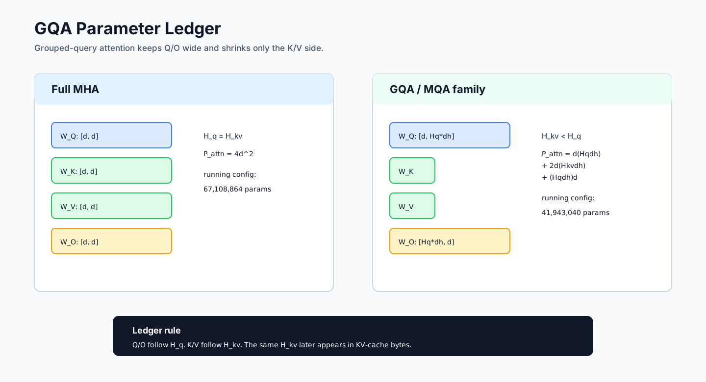
Two consequences are easy to miss:

1. Splitting a fixed packed width into more query heads does not itself create more projection parameters. The count changes when a declared packed width changes.
2. A fused QKV tensor does not automatically add parameters. If it is exactly the concatenation of Q, K, and V, its output axis is d_q+2d_kv and its scalar count is the same. Extra padding, duplicated scales, or a different packing contract must be declared separately.

GQA’s H_kv later changes K/V-cache state as well, but that is a different ledger. A static parameter saving is not a complete serving-cost claim.

0x02C MLP: Projection Count And Width Must Be Read Together

A classic ReLU/GeLU-style FFN owns two projections:

first weight:  [d_ff,d] stored      -> d*d_ff scalars
second weight: [d,d_ff] stored      -> d*d_ff scalars

Therefore:

$$P_{\text{MLP,classic,weights}}=2dd_{ff}.$$

If both linear layers have bias, the output widths add:

$$P_{\text{MLP,classic,bias}}=d_{ff}+d.$$

The original Transformer used d_ff=4d, so its two-matrix weight term is 8d^2. That ratio is an architectural choice, not the definition of an FFN.

A SwiGLU path owns gate, up, and down projections:

$$\operatorname{MLP}(x) = \left(\operatorname{SiLU}(xW_g)\odot xW_u\right)W_d.$$

The three stored matrices contain:

$$P_{\text{MLP,SwiGLU,weights}} =dd_{ff}+dd_{ff}+d_{ff}d =3dd_{ff}.$$

With bias on all three projections:

$$P_{\text{MLP,SwiGLU,bias}}=2d_{ff}+d.$$

The GLU-variants comparison reduces the gated hidden width by 2/3 when matching the three-matrix design to a two-matrix baseline. The factor follows from the budget equation:

$$3d\,d_{ff,\text{gated}} \approx 2d\,d_{ff,\text{classic}} \quad\Longrightarrow\quad d_{ff,\text{gated}} \approx\frac{2}{3}d_{ff,\text{classic}}.$$

Starting from the historical d_ff,classic=4d gives 8d/3, after which an implementation may round or deliberately choose another ratio. The checkpoint field intermediate_size remains authoritative.

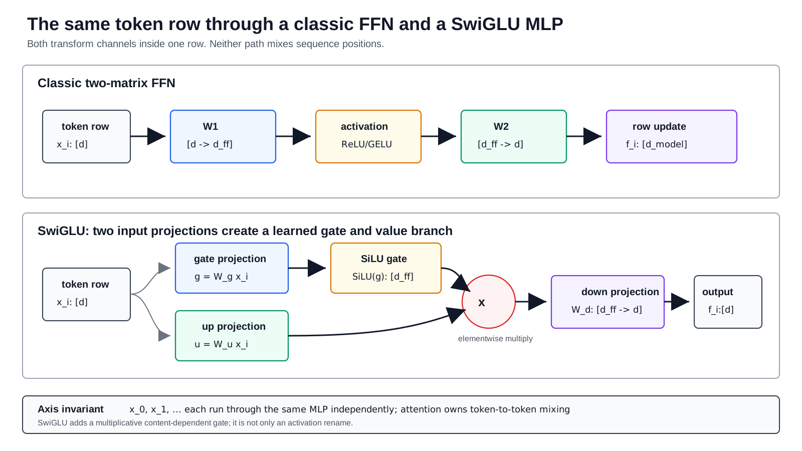
The running fixture does not use 8d/3:

d_ff / d = 14336 / 4096 = 3.5

P_MLP,weights/layer
    = 3 * 4096 * 14336
    = 176,160,768
    = 10.5d^2

The MLP has about 4.2x as many learned projection scalars as the fixture’s GQA attention path. This does not imply that it dominates activation memory or decode latency; it is only the parameter inventory.

0x02D Norms, Biases, Positions, Vocabulary, And Tying

Small terms should be explicit rather than buried in an approximation.

Normalization state

For one width-d normalization module:

$$P_{\text{RMSNorm}}=d$$

for a scale-only RMSNorm, while a scale-and-shift LayerNorm has:

$$P_{\text{LayerNorm}}=2d.$$

The running Pre-RMSNorm block owns two scale vectors, and the stack owns one final scale vector:

per block:  input_layernorm.weight          [d]
            post_attention_layernorm.weight [d]
final:      model.norm.weight               [d]

That contributes 2d per block plus d outside the stack.

Positional state

“The model has position information” does not determine a parameter count:

Position contract	Learned scalar term	Checkpoint consequence
fixed sinusoidal encoding	0	may be generated or stored as a non-parameter buffer
running RoPE fixture	0	rotation/cache state is not a learned position table in this manifest
learned absolute table with P_max rows	P_max*d	one declared trainable table
learned relative bias/table	architecture-specific	count exact stored axes and sharing policy
learned scaling or position extension	architecture-specific	must appear in the manifest and schema

The original Transformer explicitly discussed fixed sinusoidal and learned position alternatives. LLaMA removes absolute position embeddings in favor of RoPE. Neither source licenses the broader claim that every object called “rotary” or “relative” is forever parameter-free; inspect the implementation.

Vocabulary state and weight tying

The input embedding and output projection each have V*d scalar positions:

embed_tokens.weight: [V,d]
lm_head.weight:       [V,d] stored, used as [d,V] logically

Let tau=1 when the two names refer to one shared parameter object and 0 when they are independent. Let beta_U=1 when the output head has a bias. The unique vocabulary term is:

$$P_{\text{vocab,unique}} =Vd+(1-\tau)Vd+\beta_UV.$$

Thus:

untied, bias-free: 2Vd
tied, bias-free:   Vd

Weight tying is identity, not equal initialization. Copying embedding values into a separate head still leaves two trainable objects and counts twice. The output-embedding study and original Transformer motivate shared input/output weights; the running fixture explicitly sets tie_word_embeddings=false.

At V=128256 and d=4096, each independent table contains:

V*d = 128256 * 4096 = 525,336,576 scalars

Tying therefore changes this fixture-sized ledger by more than half a billion unique parameters.

0x02E One General Inventory, With Explicit Extension Hooks

For the declared decoder family, the unique count can be organized as:

$$\begin{aligned} P_{\text{total}} ={}&L\left( P_{\text{attn}} +P_{\text{MLP}} +P_{\text{norm,block}} \right) \\ &+P_{\text{token-embed}} +P_{\text{position}} +P_{\text{final-norm}} +P_{\text{head,unique}} +P_{\text{extra}}. \end{aligned}$$

P_extra is not permission to hide unknown state. It is an extension point whose members must be named and shaped:

Possible extension	What must be declared	Deeper owner
cross-attention	Q/K/V/O widths, biases, norms, and layer placement	relevant architecture article
MoE	router, routed/shared experts, expert count, sharing	M6.1-M6.2
LoRA/adapters	target modules, ranks, sharing, merge state	M6.3
multimodal projector/tower	module boundaries and whether the tower is included	X1 track
learned prefix/prompt	stored prefix rows and layer sharing	adaptation/runtime contract
quantizer scales/codebooks	logical weights versus representation metadata	M8

If the release claims to be the same base architecture but one of these objects appears in named_parameters, validation must fail until the manifest changes. Silently omitting the object is not an approximation; it is counting a different graph.

0x02F Recovering 12d^2+13d, Then Showing Its Boundary

A16’s standard dense teaching case assumes:

self-attention: MHA with d_q=d_kv=d, four biased projections
MLP:            two biased projections with d_ff=4d
normalization:  two scale-and-shift LayerNorm modules per block
vocabulary:     separate input embedding and output head
omitted:        final norm, learned positions, and all optional modules

Under precisely those assumptions:

$$\begin{aligned} P_{\text{attn}} &=4(d^2+d)=4d^2+4d, \\ P_{\text{MLP}} &=(4d^2+4d)+(4d^2+d)=8d^2+5d, \\ P_{\text{two LayerNorms}} &=2(2d)=4d. \end{aligned}$$

Therefore one block contains:

$$P_{\text{block,A16}} =12d^2+13d.$$

With L blocks and two untied vocabulary matrices, the same case gives:

$$P_{\text{A16 case}} =L(12d^2+13d)+2Vd.$$

Only after dropping the first-order and vocabulary terms does it become the mnemonic:

$$P\approx12Ld^2.$$

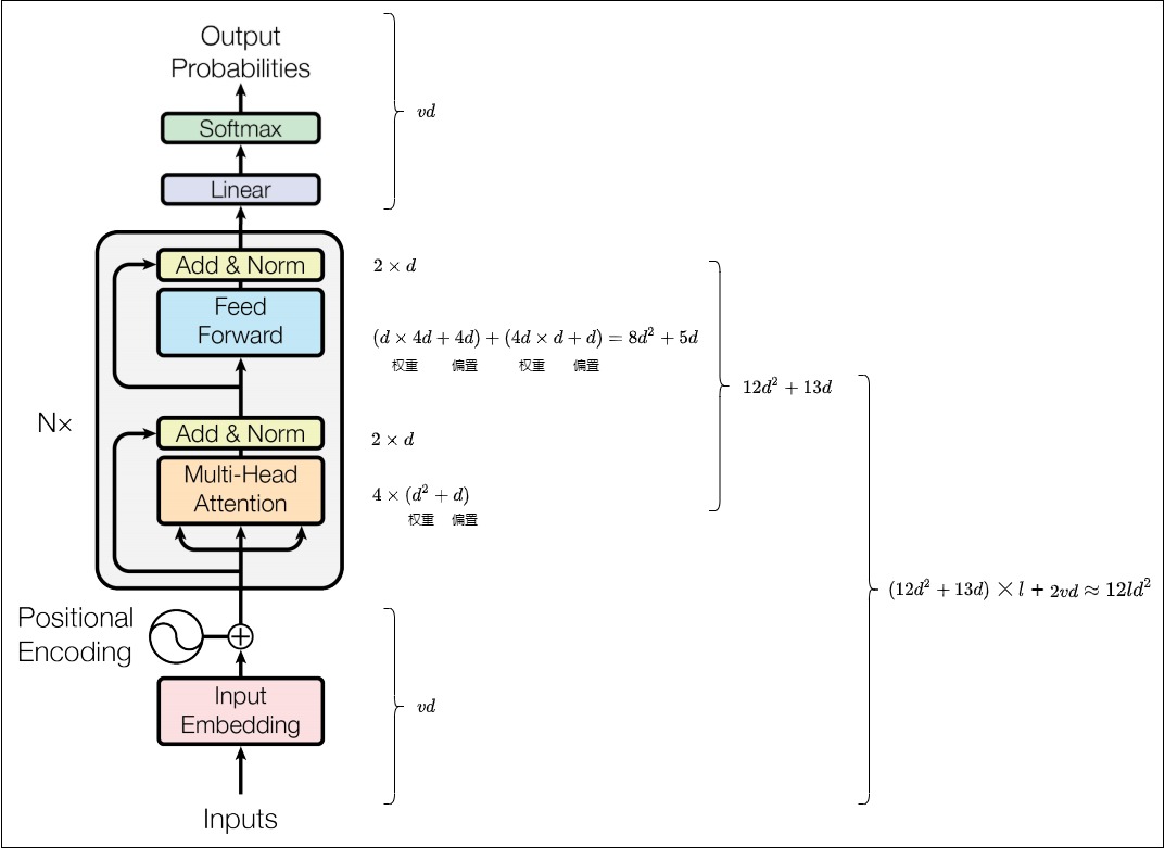
Source-local figure: author-created for A16. It illustrates A16’s declared historical architecture rather than a universal decoder inventory.

The diagram is useful because it exposes the assumptions. It is not a schema for every decoder. The original Transformer paper itself used an encoder-decoder graph, included cross-attention in decoder layers, shared embedding/pre-softmax weights, and used fixed sinusoidal positions. A16’s formula is best read as a compact dense self-attention teaching contract.

For the running fixture:

$$\begin{aligned} P_{\text{attn,weights}} &=2d^2\left(1+\frac{H_{kv}}{H_q}\right) =2d^2(1+1/4)=2.5d^2, \\ P_{\text{MLP,weights}} &=3d(3.5d)=10.5d^2. \end{aligned}$$

So the fixture’s matrix-only block is exactly:

$$P_{\text{block,matrix}}=13d^2,$$

before adding its two RMSNorm vectors. The GQA saving does not preserve the old coefficient because this fixture allocates a wider SwiGLU intermediate than the parameter-matched 8d/3 construction.

The coefficient is an output of the architecture manifest. It is not a family name and should never be used to overwrite a checkpoint’s actual dimensions.

0x02G A Manual Toy Model That Fits On One Screen

Before trusting billion-scale arithmetic, use a tiny manifest whose entire inventory can be inspected manually:

L=2, d=8, H_q=4, H_kv=2, d_h=2, d_ff=12, V=16
SwiGLU, two RMSNorms/block, final RMSNorm
no projection bias, no learned position table, untied embedding/head

The derived widths are d_q=8 and d_kv=4. One block contains:

Stored object family	Calculation	Scalars
Q and O	2 * 8 * 8	128
K and V	2 * 8 * 4	64
gate, up, down	3 * 8 * 12	288
two RMSNorm scales	2 * 8	16
one block	128+64+288+16	496

The complete model is:

Category	Calculation	Scalars
two blocks	2 * 496	992
token embedding	16 * 8	128
untied output head	16 * 8	128
final RMSNorm	8	8
unique total	992+128+128+8	1,256

If the output head is tied to the token embedding, the named schema can still contain both paths, but the unique total becomes:

1,256 - 128 = 1,128 unique scalars

This toy is small enough to catch an omitted final norm, accidental bias, wrong K/V width, or tied-weight double count immediately.

0x02H Independent Analytical And Runtime Counts

The analytical path must not call model.parameters(). It derives a number from manifest fields and architecture rules:

def analytic_fixture_count(m):
    assert m.attention_bias is False
    assert m.mlp_bias is False
    assert m.tie_word_embeddings is False

    d_q = m.num_attention_heads * m.head_dim
    d_kv = m.num_key_value_heads * m.head_dim

    attention = 2 * m.hidden_size * d_q + 2 * m.hidden_size * d_kv
    swiglu = 3 * m.hidden_size * m.intermediate_size
    block_norms = 2 * m.hidden_size
    block = attention + swiglu + block_norms

    token_embedding = m.vocab_size * m.hidden_size
    output_head = m.vocab_size * m.hidden_size
    final_norm = m.hidden_size

    return (
        m.num_layers * block
        + token_embedding
        + output_head
        + final_norm
    )

The observed path inspects module objects independently. It records aliases, unique learned scalars, currently trainable scalars, state-entry scalars, and persistent buffers as separate evidence:

from collections import OrderedDict

def observe_parameter_inventory(model):
    groups = OrderedDict()
    named_occurrence_numel = 0

    for name, parameter in model.named_parameters(remove_duplicate=False):
        named_occurrence_numel += parameter.numel()
        row = groups.setdefault(
            id(parameter),
            {"parameter": parameter, "aliases": []},
        )
        row["aliases"].append(name)

    unique_numel = sum(row["parameter"].numel() for row in groups.values())
    trainable_numel = sum(
        row["parameter"].numel()
        for row in groups.values()
        if row["parameter"].requires_grad
    )

    state = model.state_dict()
    state_entry_numel = sum(tensor.numel() for tensor in state.values())
    persistent_buffer_numel = sum(
        tensor.numel()
        for name, tensor in model.named_buffers()
        if name in state  # non-persistent buffers have no state_dict entry
    )

    return {
        "unique_parameter_numel": unique_numel,
        "trainable_parameter_numel": trainable_numel,
        "named_parameter_occurrence_numel": named_occurrence_numel,
        "state_entry_numel": state_entry_numel,
        "persistent_buffer_numel": persistent_buffer_numel,
        "aliases": [row["aliases"] for row in groups.values()],
    }

expected = analytic_fixture_count(manifest)
observed = observe_parameter_inventory(model)

assert observed["unique_parameter_numel"] == expected
assert observed["trainable_parameter_numel"] == expected  # fixture: all trainable

The schema validator in 0x01 and the count reconciliation here answer different questions:

schema validation:
    are the expected names, optional terms, shapes, dtypes, and aliases present?

count reconciliation:
    does an independent object traversal sum to the analytical inventory?

Both are required. Two wrong shapes can preserve the same total. A correct schema can still be double-counted when aliases are summed by name.

0x02I Exact Running Ledger

Applying the equations to m4.1-dense-gqa-swiglu-v1 gives:

Category	Per-layer or external count	Multiplicity	Total scalars
Q/K/V/O weights	41,943,040	32 layers	1,342,177,280
SwiGLU weights	176,160,768	32 layers	5,637,144,576
two RMSNorm scales	8,192	32 layers	262,144
token embedding	525,336,576	1	525,336,576
untied output head	525,336,576	1	525,336,576
final RMSNorm	4,096	1	4,096
unique learned scalars			8,030,261,248

The arithmetic closes by independent groups:

matrix weights inside blocks:
    32 * (41,943,040 + 176,160,768)
    = 6,979,321,856

all learned norm scales:
    32 * 8,192 + 4,096
    = 266,240

untied vocabulary matrices:
    2 * 525,336,576
    = 1,050,673,152

total:
    6,979,321,856 + 266,240 + 1,050,673,152
    = 8,030,261,248

This is an 8.030B-scalar analytical teaching fixture, not a claim that a particular released file or marketing label must have this exact count. A tied version of the same schema would contain 7,504,924,672 unique scalars. A version with biases, another vocabulary, another intermediate_size, learned positions, or extra modules is a different manifest.

0x02J Parameter Failure Lab And Publish Gate

Failure	Incorrect result	Required invariant
insert B, S, or T into the learned-weight count	workload-dependent parameter total	architecture state is independent of workload extents
assume all four attention matrices are [d,d]	GQA/MQA K/V overcount	derive d_q and d_kv separately
infer d_ff=4d or 8d/3 from an activation label	wrong MLP count	read stored projection count and intermediate_size
omit biases because they are small	schema mismatch	count output-axis bias vectors when enabled
count RoPE cache/state as learned weights	parameter overcount	distinguish parameters from generated or persistent buffers
omit final norm or learned position tables	undercount	enumerate every declared outside-stack object
treat equal embedding/head values as tied	undercount	verify object/storage identity
sum alias names or state_dict entries as unique parameters	tied-weight or buffer overcount	deduplicate parameters and report buffers separately
count only requires_grad=True	frozen learned state disappears	report unique learned and currently trainable counts separately
multiply a local tensor-parallel shard by no ownership rule	global/local ambiguity	bind the ownership policy before reconciliation
hide experts, adapters, or projectors in P_extra	count describes another graph	name, shape, and assign every extension

The parameter ledger is ready to feed 0x03 only when:

all stored axes follow the declared source implementation
every optional state family is included or explicitly absent
tied aliases are identity-checked
the exact toy count equals the observed tiny model count
the running analytical total equals an independent unique-parameter traversal
12Ld^2 is labeled as a recovered special case, not a universal law

0x03 Numerical Representation And Persistent Training State

The parameter ledger in 0x02 counted logical learned scalars. It did not say how many physical tensor copies exist, which data type stores each copy, where those tensors live, or during which phase they are present. Those choices turn a parameter count into a memory inventory.

The owner question is therefore narrower than “how much memory does training use?”:

For one declared set of learned parameters, which model, master, gradient, optimizer, and auxiliary state objects exist under a named policy, and how many bytes does each object contribute while it is live?

This section owns the global single-rank state inventory. It does not yet divide objects across ranks, derive activation peaks, or explain low-bit number formats:

owned here:
    learned-parameter representation
    master/update copies
    gradient storage
    optimizer slots and scalar metadata
    object creation and release boundaries
    checkpoint-versus-resident-state distinction

deferred:
    activation liveness and allocator peak             -> 0x04
    per-rank ZeRO/FSDP/TP/PP ownership and gathers     -> 0x07
    quantizer codes, scales, packing, and kernel path  -> M8
    adapter-specific trainable-state policies          -> M6.3

0x03A A State Ledger Is A Sum Over Named Objects

Let state class j have scalar count C_j, copy count r_j, storage data type with b_j bytes per scalar, placement pi_j, and a lifetime indicator a_j(tau) that is one when the object is live at execution point tau. The logical payload at one placement is:

$$M_{\text{state}}^{(\pi)}(\tau) = \sum_j \mathbf 1[\pi_j=\pi]\, a_j(\tau)\,r_jC_jb_j +M_{\text{metadata}}^{(\pi)}(\tau).$$

This is intentionally not P times one multiplier. Each row needs an object contract:

Field	Question it answers
role	Is this a model parameter, master copy, gradient, first moment, second moment, step scalar, scale, or other state?
count rule	Does it have P_loaded, P_train, one value per matrix row/column, one scalar per tensor, or another shape?
dtype	How many bytes does the stored representation require per element?
copies	Is there one object, a working and master pair, or another replica?
placement	GPU, CPU, NVMe, checkpoint artifact, or multiple locations?
created	Model load, first backward, first optimizer step, or checkpoint materialization?
released	Never during the run, after zero_grad, after the step, or after serialization?
owner	Model module, autograd, optimizer, distributed wrapper, scaler, or checkpoint runtime?

Two parameter populations matter:

P_loaded:
    unique learned scalars that must be represented for the forward graph

P_train:
    subset that receives gradients and optimizer state under this run policy

If a fraction f of loaded parameters is trainable, then P_train=fP_loaded. Freezing does not remove the base weight bytes. It can remove gradient and optimizer-state terms if no stale state is loaded for those parameters.

A generic dense-state ledger is:

$$\begin{aligned} M_{\text{model}} &= P_{\text{loaded}}b_w,\\ M_{\text{master}} &= P_{\text{master}}b_m,\\ M_{\text{grad}}(\tau) &= P_{\text{grad}}(\tau)b_g,\\ M_{\text{optimizer}}(\tau) &=\sum_{s\in\mathcal S_{\text{opt}}}C_s(\tau)b_s,\\ M_{\text{declared}}(\tau) &=M_{\text{model}}+M_{\text{master}}+M_{\text{grad}}(\tau) +M_{\text{optimizer}}(\tau)+M_{\text{aux}}(\tau). \end{aligned}$$

The equation reports tensor payload. Storage padding, allocator reserve, temporary optimizer intermediates, communication buckets, and kernel workspace remain separate observations.

0x03B Representation Is Not The Same Thing As Compute Precision

For a dense uncompressed tensor, bytes follow directly from its stored dtype:

$$M(W)=\operatorname{numel}(W)\operatorname{element\_size}(W).$$

For one billion scalar positions:

Stored representation	Payload bytes	Decimal GB	Binary GiB	Boundary
fp32	4,000,000,000	4.00	3.73	one dense fp32 tensor
fp16 or bf16	2,000,000,000	2.00	1.86	one dense 16-bit tensor
fp8 or int8 codes	1,000,000,000	1.00	0.93	excludes scaling and layout metadata
packed int4 codes	500,000,000	0.50	0.47	excludes scales, zero-points, padding, and exceptions

The last two rows are only code-payload lower bounds. M8.1 derives why effective bits must include group metadata and why a compact checkpoint is not automatically a compact runtime tensor.

The word compute names something else. PyTorch autocast chooses operation dtypes inside an autocast region. That does not, by itself, prove that the model owns an additional persistent fp16 weight tensor or an fp32 master tensor. Conversely, a training system can deliberately keep a low-precision working copy plus a higher-precision master copy. The object inventory, not the phrase “mixed precision,” decides the byte ledger.

stored parameter dtype:
    representation of the long-lived model tensor

operator input/accumulator dtype:
    execution choice for one kernel

autocast cache or converted tile:
    implementation-managed state with its own lifetime

master parameter:
    explicit high-precision state updated by the optimizer

These objects can have different dtypes and lifetimes even when they participate in the same training step.

0x03C Why A Master Weight Can Exist

The original Mixed Precision Training method stored weights, activations, and gradients in fp16 while maintaining one fp32 copy of the weights for updates. The low-precision working weights were regenerated by rounding the updated fp32 master weights.

The numerical reason is visible near one. Adjacent representable values in [1,2) are separated approximately by:

bf16: 2^-7  = 0.0078125
fp16: 2^-10 = 0.0009765625
fp32: 2^-23 ~= 0.0000001192

An update of magnitude 1e-4 applied directly to a weight near 1 can round away in bf16 and fp16. Accumulating the update in fp32 preserves it until the rounded working copy moves to another representable low-precision value. This motivates a master copy; it does not prove that every modern bf16 runtime uses one. Numerical formats and update-stagnation mechanisms are developed more deeply in M8.

A paper-style working/master step is:

def mixed_precision_update(model_fp16, master_fp32, grad_fp16, optimizer_state):
    grad_fp32 = cast_fp32(unscale_if_needed(grad_fp16))
    master_fp32, optimizer_state = optimizer_step(
        master_fp32,
        grad_fp32,
        optimizer_state,
    )
    model_fp16.copy_(round_to_fp16(master_fp32))

That code declares two parameter objects and, temporarily or persistently, two gradient representations. A PyTorch autocast loop with fp32 parameters has a different inventory even if many GEMMs execute in fp16.

0x03D Derive Optimizer Slots From The Update Rule

Optimizer memory is not an arbitrary multiplier. It follows from state carried between steps.

Adam maintains first- and second-moment estimates:

$$m_t=\beta_1m_{t-1}+(1-\beta_1)g_t,$$ $$v_t=\beta_2v_{t-1}+(1-\beta_2)g_t^2.$$

Both recurrences need the previous full-shape value at the next step. For P_train trainable scalar positions, ordinary dense Adam therefore has:

$$C_m=P_{\text{train}}, \qquad C_v=P_{\text{train}}.$$

With fp32 moments:

$$M_{\text{Adam moments}} =4P_{\text{train}}+4P_{\text{train}} =8P_{\text{train}}\ \text{bytes}.$$

AdamW changes how weight decay is applied; it does not require a third full-size state tensor. AMSGrad does: it retains the running maximum of the second moment, adding another P_train-sized slot.

Optimizer family	Long-lived full-shape slot contract	Dense auxiliary scalar count
SGD without momentum	none	0
momentum SGD	momentum buffer	P_train
Adam / AdamW	first moment m, second moment v	2P_train
AMSGrad	m, v, maximum second moment	3P_train

The official PyTorch Adam source makes another implementation detail visible: state is initialized lazily, only when a parameter with a gradient reaches an optimizer step. It creates exp_avg, exp_avg_sq, and a step tensor; with AMSGrad it also creates max_exp_avg_sq. In that implementation the moments are created with zeros_like(parameter), so their dtype follows the actual parameter object unless a wrapper or optimizer policy changes it.

Consequently, this statement is unsafe:

bf16 model + AdamW automatically means fp32 moments

The safe statement is:

inspect the optimizer state after initialization,
then record every slot's actual shape, dtype, and placement

0x03E Recovering The Source-Local 20-Byte Policy

A16 gives the following teaching diagram:

Source-local figure: author-created for A16. The six-object state policy is an accounting example and is not attributed to every mixed-precision runtime.

Read it as an object inventory, not as a universal execution timeline. Its declared objects are:

State object	Count	Bytes/scalar	Contribution per trainable parameter
low-precision working parameter	P_train	2	2 bytes
fp32 master/update parameter	P_train	4	4 bytes
low-precision gradient	P_train	2	2 bytes
fp32 gradient/update copy	P_train	4	4 bytes
fp32 Adam first moment	P_train	4	4 bytes
fp32 Adam second moment	P_train	4	4 bytes

Therefore:

$$\begin{aligned} M_{\text{A16 policy}} &=P_{\text{train}}(2+4+2+4+4+4)\\ &=20P_{\text{train}}\ \text{bytes}. \end{aligned}$$

The arithmetic is correct for that declared six-object policy. The coefficient is not a property of AdamW or mixed precision in isolation. For example, a runtime may cast one gradient into fp32 transiently instead of retaining both gradient copies, keep fp32 parameters under autocast with no separate master, or store moments in the parameter dtype.

Equal coefficients can also hide different objects:

fp32 parameter + fp32 gradient + fp32 Adam m/v:
    4 + 4 + 4 + 4 = 16 bytes/parameter

bf16 working parameter + fp32 master + bf16 gradient + fp32 Adam m/v:
    2 + 4 + 2 + 4 + 4 = 16 bytes/parameter

Both total 16 bytes per trainable parameter, but only the second policy owns a separate working/master pair. A byte total cannot substitute for a state schema.

0x03F Exact Running-Fixture State Ledgers

The 0x02 running fixture contains:

P_loaded = P_train = 8,030,261,248 unique scalars
single-rank global inventory
no sharding or offload
gradients are live where the row includes them
Adam moments have already been initialized
activations, workspace, allocator reserve, and K/V are excluded

The same model produces several valid state totals:

Policy	Named payload per parameter	Bytes/parameter	Decimal GB	Binary GiB
bf16 inference weights	working weight 2	2	16.061	14.958
fp32 inference weights	model weight 4	4	32.121	29.915
masterless bf16 + bf16 grad + fp32 m/v	2+2+4+4	12	96.363	89.745
fp32 parameters under autocast + fp32 grad + fp32 m/v	4+4+4+4	16	128.484	119.660
bf16 working + fp32 master + bf16 grad + fp32 m/v	2+4+2+4+4	16	128.484	119.660
A16 dual-parameter, dual-gradient, fp32-Adam policy	2+4+2+4+4+4	20	160.605	149.575

The masterless bf16 row is an accounting policy, not a training recommendation or a claim about vanilla PyTorch AdamW. Every row must be tied to an implementation that actually creates the listed objects.

For a partially trainable model, full base-weight storage remains while trainable-only state scales with f:

$$M =P_{\text{loaded}}b_w +fP_{\text{loaded}} \left(b_m+b_g+\sum_sb_s\frac{C_s}{P_{\text{train}}}\right) +M_{\text{aux}}.$$

M6.3 applies this distinction to adapters. M4.1 only establishes the accounting contract.

0x03G State Is Created At Different Times

Calling an optimizer constructor does not necessarily allocate every parameter-sized state tensor. A representative PyTorch Adam lifecycle is:

after model load:
    model parameters exist
    gradients may be None

after optimizer construction, before any step:
    parameter groups and hyperparameters exist
    per-parameter m/v state can still be absent

after backward:
    gradients exist for parameters that participated and require gradients

during the first optimizer step:
    Adam lazily creates step, exp_avg, and exp_avg_sq for parameters with grads

after zero_grad(set_to_none=True):
    .grad references become None
    allocator-reserved device memory need not fall by the same byte count

PyTorch documents that zero_grad(set_to_none=True) generally has a lower memory footprint than writing zeros and changes optimizer behavior for None versus zero gradients. This is an object-lifetime statement, not a guarantee that a caching allocator immediately returns memory to the driver.

This timing explains two common measurement discrepancies:

measure before first optimizer.step():
    Adam moments may not exist yet -> optimizer state is undercounted

measure device free memory after grad=None:
    logical gradient tensors may be gone while allocator reserve remains

Section 0x04 derives liveness and analytical peak more generally. Here the important point is that even “persistent training state” has creation and release boundaries.

0x03H Alternative Optimizers Change Shape As Well As Dtype

Reducing optimizer memory is not limited to storing the same two Adam slots in fewer bits.

Adafactor: change the state geometry

For a matrix parameter W with shape [r,c], a dense second moment stores rc values. Adafactor approximates that state from row and column statistics, requiring r+c values:

$$C_{v,\text{dense}}=rc, \qquad C_{v,\text{factored}}=r+c.$$

For the running fixture’s gate_proj.weight with shape [14336,4096]:

dense second moment:
    14336 * 4096 = 58,720,256 values

factored row + column state:
    14336 + 4096 = 18,432 values

ratio for this slot:
    18,432 / 58,720,256 ~= 0.0003139

Vectors and matrices that are not factored need their own rules. Optional momentum can restore a full first-moment slot. “Adafactor uses almost no state” is therefore still incomplete without the parameter-shape and momentum policy.

Eight-bit Adam: retain the slots, change their representation

The 8-bit Optimizers paper keeps Adam-like statistics but stores them through block-wise dynamic quantization. Its update path dequantizes state values for computation and requantizes them for storage; block metadata and selected fp32 exceptions remain part of the physical inventory.

A lower-bound sketch is:

$$M_{\text{two 8-bit slots}} \gtrsim 2P_{\text{train}}\ \text{bytes} +M_{\text{block metadata}} +M_{\text{fp32 exceptions}}.$$

This is not 2P exactly, and the paper’s quantization method cannot be replaced with arbitrary linear uint8 storage while retaining its claims. M8 owns the code, scale, block, and kernel details; M4.1 records the resulting state objects.

The two methods answer different questions:

Method	What changes	What must still be declared
Adafactor	second-moment shape, optionally first-moment existence	matrix/vector factoring policy, momentum, dtype
8-bit Adam	representation of Adam-like slots	code format, block metadata, exceptions, update path
ZeRO/FSDP	per-rank ownership of global state	shard degree, transient gathers, communication, offload

The last row is derived in 0x07: sharding does not reduce the global logical state described in this section.

0x03I Resident State, Optimizer State, And Checkpoint State Are Different

PyTorch’s optimizer state_dict contains per-parameter optimizer state and parameter-group metadata; it does not contain the parameter tensors themselves. A restartable training checkpoint usually combines several independently owned objects:

model state:
    parameters and persistent model buffers

optimizer state:
    moments, step counters, parameter-group metadata

training-control state:
    scheduler, gradient scaler, global step, sampler position

reproducibility state when required:
    RNG states and data-pipeline cursor/manifest

Gradients are not automatically included merely because they were live on the device. Frameworks can shard, flatten, offload, stage, or encode checkpoint tensors differently from runtime storage. Therefore:

GPU resident tensor payload
    != process allocated/reserved memory
    != global distributed state
    != serialized checkpoint bytes

An exact report keeps these ledgers separate and states whether temporary serialization buffers are included in peak memory.

0x03J Observe The State Independently

The analytical policy should be reconciled against live objects after the intended lifecycle point. The following is pseudocode: wrappers can own master weights or flattened shards outside both the model and optimizer, so their registries must be added explicitly.

def tensor_payload(t):
    return t.numel() * t.element_size()


def observe_training_state(model, optimizer, wrapper_state=()):
    rows = []

    # model.parameters() normally deduplicates tied Parameter objects
    for name, p in model.named_parameters(remove_duplicate=True):
        rows.append(record(
            role="model_parameter",
            name=name,
            shape=tuple(p.shape),
            dtype=p.dtype,
            device=p.device,
            logical_bytes=tensor_payload(p),
        ))
        if p.grad is not None:
            rows.append(record(
                role="gradient",
                name=f"{name}.grad",
                shape=tuple(p.grad.shape),
                dtype=p.grad.dtype,
                device=p.grad.device,
                logical_bytes=tensor_payload(p.grad),
            ))

    for parameter, slots in optimizer.state.items():
        parameter_name = unique_name_for_parameter(parameter)
        for slot_name, value in slots.items():
            if is_tensor(value):
                rows.append(record(
                    role=f"optimizer.{slot_name}",
                    name=parameter_name,
                    shape=tuple(value.shape),
                    dtype=value.dtype,
                    device=value.device,
                    logical_bytes=tensor_payload(value),
                ))
            else:
                rows.append(record_non_tensor_metadata(slot_name, value))

    rows.extend(observe_wrapper_owned_tensors(wrapper_state))
    return group_by_role_dtype_device(rows)

The reconciliation gate is schema-first:

def reconcile_state_policy(policy, observed, lifecycle_point):
    expected = derive_expected_state_rows(policy, lifecycle_point)

    assert expected.roles == observed.roles
    assert expected.shape_multiset == observed.shape_multiset
    assert expected.dtype_by_role == observed.dtype_by_role
    assert expected.device_by_role == observed.device_by_role
    assert expected.logical_bytes_by_role == observed.logical_bytes_by_role

Do not validate only the grand total. Two missing bf16 objects can be masked by one accidental fp32 object. Also do not measure Adam immediately after construction if the policy expects initialized moments.

0x03K Persistent-State Failure Lab And Publish Gate

Failure	Hidden mistake	Consequence
mixed precision = 16 bytes/P	no object schema was declared	coefficient may fit the wrong runtime
count autocast as a permanent fp16 model copy	operation dtype confused with persistent state	model bytes double-counted
assume bf16 parameter implies fp32 Adam slots	optimizer implementation not inspected	state dtype and bytes wrong
inspect Adam before its first step	lazy m/v state not initialized	optimizer memory undercounted
count all parameters as trainable	P_loaded confused with P_train	gradients and state overcounted
omit frozen base weights	no gradients mistaken for no storage	resident model undercounted
call grad=None equivalent to driver memory release	tensor lifetime confused with allocator reserve	measured free memory does not match formula
treat Adafactor as a dtype-only variant	state geometry ignored	matrix-dependent savings lost
write 2P for 8-bit Adam	metadata and exceptions omitted	physical state undercounted
divide by world size here	global state confused with rank ownership	later ownership contract bypassed
equate checkpoint bytes with GPU state	serialization and placement ignored	restart artifact mis-sized

Publish gate:

every byte belongs to a named object with count, dtype, copies, placement, and lifetime
P_loaded and P_train are distinct
compute dtype is not used as evidence for persistent copies
Adam's two moments are derived from its recurrences
the A16 20-byte case is recovered exactly and scoped as one policy
12-, 16-, and 20-byte totals expose their different state schemas
lazy initialization and grad=None timing are explicit
optimizer alternatives distinguish changed shape from changed representation
global state is not divided before the parallel-ownership section
checkpoint bytes are not called resident GPU memory

0x04 Activation Liveness, Peak Memory, And Recomputation

The parameter and optimizer ledgers describe objects that survive for long intervals. Activations are different. A tensor may exist for one operator, be retained until a distant backward operator, be reconstructed instead of saved, or share storage with another tensor view. Its contribution depends on when it is live, not only on its shape.

The owner question is:

Which unique storages must coexist at each point in forward and backward, which of them are retained for gradient computation, and how does a declared recomputation or offload policy change the peak?

This section owns the unsharded logical activation inventory and its observation contract:

owned here:
    forward temporaries and saved-for-backward tensors
    birth, last use, and release boundaries
    logical live-payload and peak-cut equations
    workspace, allocated, reserved, and external-memory distinctions
    A16/Korthikanti coefficient reconstruction
    no, selective, full-region, and offload policies

deferred:
    exact extra forward/backward FLOPs                 -> 0x05 and later compute loop
    per-rank TP/SP/CP/PP ownership and communication  -> 0x07
    tiled attention's custom forward/backward schedule -> M4.3
    activation quantization and compression formats   -> M8

0x04A An Activation Is A Backward Dependency, Not Every Forward Output

Consider one pre-norm decoder block as an execution graph:

x
 -> norm_1
 -> q, k, v
 -> scores
 -> probabilities
 -> context
 -> output projection
 -> residual_1
 -> norm_2
 -> gate, up
 -> silu(gate) * up
 -> down projection
 -> residual_2

Every arrow is a mathematical value. It does not follow that every value owns a distinct persistent allocation or must be retained until backward. The backward formulas decide which information is needed.

For a linear map Y = XW, reverse-mode differentiation gives:

$$\frac{\partial \mathcal L}{\partial X} = \frac{\partial \mathcal L}{\partial Y}W^T, \qquad \frac{\partial \mathcal L}{\partial W} = X^T\frac{\partial \mathcal L}{\partial Y}.$$

The weight-gradient path needs X; the input-gradient path needs W. It does not generally need Y. An autograd implementation may therefore save the linear input rather than its output.

For row-wise softmax p = softmax(z), the vector-Jacobian product can be written:

$$\frac{\partial \mathcal L}{\partial z} = p\odot \left( \frac{\partial \mathcal L}{\partial p} - \left\langle \frac{\partial \mathcal L}{\partial p},p \right\rangle\mathbf 1 \right).$$

Backward needs the probabilities p, or enough information and compute to reconstruct them. Dropout needs the keep/drop decision, which can be represented as a mask or reproduced from an exact RNG contract. A SwiGLU branch

$$h=\operatorname{SiLU}(g)\odot u, \qquad g=xW_g, \qquad u=xW_u$$

needs enough state to recover derivatives through both SiLU(g) and the elementwise product. An implementation can save x, g, and u, save a different equivalent set, fuse some state, or recompute part of the branch.

This produces four distinct object roles:

Role	Why it exists	Typical release boundary
forward temporary	consumed by a nearby forward operator	after final forward use
saved tensor	required by a later backward formula	after its backward consumer, unless graph retained
checkpoint boundary	input needed to rerun a discarded region	after region backward
backward temporary	gradient, reduction, or workspace created during reverse execution	after its backward consumers finish

PyTorch’s autograd documentation makes the contract explicit: operators save selected tensors for backward; the graph itself is not a second copy of every activation. The exact saved set is operator-, fusion-, and version-dependent.

0x04B Trace The Executable Block Before Counting

A16 follows the Megatron-style block and core-attention region shown below. The red dashed boundary is important: it identifies the post-projection attention subgraph targeted by the paper’s selective recomputation policy.

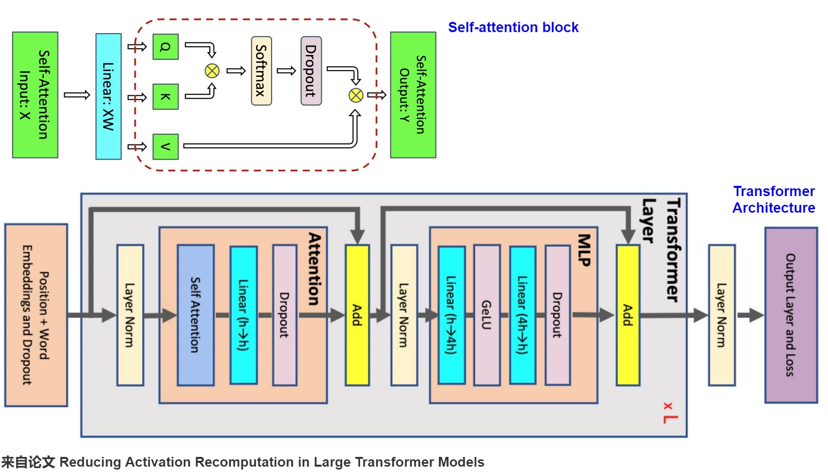
Source figure: Korthikanti et al., Reducing Activation Recomputation in Large Transformer Models, Figures 2 and 3, combined in A16. Reproduced for technical commentary; rights remain with the authors or publisher. The architecture and selected region retain the paper’s MHA, GeLU, LayerNorm, and dropout assumptions.

For a concrete implementation, build a trace row for every storage rather than starting from a coefficient:

Storage family	Logical shape	Backward reason	Linear or quadratic in s?
residual/norm input	[b,s,h]	residual and norm gradients	linear
Q	[b,a,s,h/a]	score gradient	linear
K/V in paper MHA case	[b,a,s,h/a] each	score and value-mix gradients	linear
attention score/probability	[b,a,s,s]	softmax and value-mix gradients	quadratic
attention dropout state	[b,a,s,s] in the paper policy	replay dropout	quadratic
MLP intermediates	[b,s,4h] in the paper GeLU block	activation and linear gradients	linear

The running manifest is not identical to that paper case. It declares GQA with H_kv=8, SwiGLU with d_ff=14336, RMSNorm, and a Llama-like dropout policy. Its exact saved set must be obtained from its actual operators. Replacing those choices with a MHA heads, a 4h GeLU MLP, and byte-per-element dropout masks would silently count a different architecture.

The obvious attention shapes still expose the potential cliff:

Q: [B, H_q, S_q, d_h]
K: [B, H_kv, S_k, d_h]
V: [B, H_kv, S_k, d_h]

S_attn = Q @ K.T:       [B, H_q, S_q, S_k]
P_attn = softmax(S):    [B, H_q, S_q, S_k]

For full prefill self-attention, S_q=S_k=S. In the running dimensions one materialized fp16/bf16 score tensor is:

elements = 1 * 32 * 4096 * 4096
         = 536,870,912

payload  = 536,870,912 * 2 bytes
         = 1,073,741,824 bytes
         = 1.00 GiB

A separate probability tensor contributes another 1.00 GiB. A byte-per-entry dropout mask contributes 0.50 GiB. Whether all three are simultaneously live, aliased, fused, or saved is an execution-policy question.

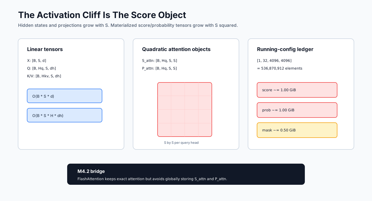
0x04C Liveness Is An Interval And Peak Is A Cut

For each unique storage i, record payload m_i, birth event u_i, and the event after its final use v_i. With half-open intervals [u_i,v_i), logical live activation payload at event tau is:

$$M_{\text{activation}}(\tau) = \sum_i m_i\mathbf 1[u_i\leq\tau<v_i].$$

The activation peak is the maximum cut through those intervals:

$$M_{\text{activation,peak}} = \max_\tau M_{\text{activation}}(\tau).$$

The full logical process payload also includes objects from other ledgers:

$$\begin{aligned} M_{\text{logical}}(\tau) ={}&M_{\text{persistent}}(\tau) +M_{\text{activation}}(\tau) +M_{\text{gradient}}(\tau)\\ &+M_{\text{workspace}}(\tau) +M_{\text{communication}}(\tau). \end{aligned}$$

The maximum of each category cannot be added independently unless those maxima occur at the same event. The correct process peak is:

$$M_{\text{logical,peak}}=\max_\tau M_{\text{logical}}(\tau).$$

An adversarial toy ledger shows why summing all objects is wrong:

Object	Payload	Live interval
persistent model/training state	20 GiB	entire step
saved residual A	4 GiB	[0,4)
attention temporary B	5 GiB	[1,2)
kernel workspace W	3 GiB	[1.5,1.8)
later backward gradient C	6 GiB	[2,3)

The non-persistent object sizes sum to 18 GiB. They never coexist. Their peak is A+B+W=12 GiB, so the logical process peak is 32 GiB, not 38 GiB. This result assumes release-at-2 is processed before birth-at-2. A real trace must preserve the runtime’s event and stream ordering rather than inventing that order later.

0x04D Logical Payload, Allocator State, And Device Use

Five measurements answer different questions:

Quantity	What it includes	What it does not prove
saved-tensor payload	unique storages retained for backward	instantaneous peak or workspace
logical live payload	declared live storages at one event	allocator rounding or external libraries
allocated bytes	live allocations managed by the framework allocator	bytes reserved but currently inactive
reserved bytes	allocator segments retained for reuse	all device memory used outside that allocator
device-used bytes	process/runtime/device use visible to a lower-level observer	which tensor or operator owns each byte

For the PyTorch CUDA caching allocator:

max_memory_allocated(): peak bytes occupied by tensors tracked by the allocator
max_memory_reserved():  peak bytes held in allocator-managed segments
memory_snapshot():      segment, block, state, and optional allocation history

Normally reserved >= allocated, but neither value is the analytical activation ledger. Views must be deduplicated by storage, allocator blocks can exceed the requested payload, asynchronous frees can remain active-awaiting-free, and workspace can overlap saved activations. PyTorch also documents that its CUDA snapshot does not see allocations made outside its allocator; NCCL is a common example.

The observation stack is therefore:

derive unique tensor-storage payload from the execution contract
measure allocator allocated and reserved peaks after warmup
capture an allocation-history snapshot around the measured step
compare lower-level device use for allocations outside the framework allocator
report the residual instead of assigning it to "activations"

0x04E Reconstruct The A16/Korthikanti Coefficients

The paper defines activation memory as forward-created tensors necessary for gradient computation. It assumes:

b = microbatch size on the considered worker
s = sequence length
h = hidden width
a = attention heads
classic MHA with Q, K, and V width h
GeLU MLP with intermediate width 4h
fp16 activations at 2 bytes per element
dropout masks at 1 byte per element
small layer-norm mean/variance buffers omitted
no model parallelism in the first formula

The attention coefficient can be rebuilt one row at a time:

Saved object in the paper contract	Byte term	Reason
shared Q/K/V projection input	2bsh	projection weight gradients
Q and K	4bsh	QK^T backward
softmax output	2bas^2	softmax backward
softmax-dropout mask	bas^2	dropout replay
dropout output and V	2bas^2 + 2bsh	value-mix backward
output-projection input	2bsh	output weight gradient
output-dropout mask	bsh	residual dropout replay
attention total	11bsh + 5bas^2	linear plus quadratic state

The MLP and normalization terms are:

Saved object in the paper contract	Byte term
first MLP linear input	2bsh
GeLU input at width 4h	8bsh
second MLP linear input at width 4h	8bsh
MLP dropout mask	bsh
two LayerNorm inputs	4bsh
MLP plus norms	23bsh

Therefore:

$$\begin{aligned} M_{\text{attention}} &= 11bsh+5bas^2,\\ M_{\text{MLP}} &= 19bsh,\\ M_{\text{two norms}} &= 4bsh,\\ M_{\text{layer,A16}} &= 34bsh+5bas^2. \end{aligned}$$

For L layers, while ignoring embeddings, final normalization, loss state, and pipeline schedule effects, the paper’s no-parallelism approximation is:

$$M_{\text{stack,A16}}=L(34bsh+5bas^2).$$

The coefficient 34 is not Transformer topology. It is the sum of saved-object bytes under this architecture and operator policy. The coefficient 5 is the same kind of policy for the three quadratic attention objects.

0x04F A Policy Projection On The Running Dimensions

Applying the A16 assumptions to the running dimensions is useful as a counterfactual sensitivity calculation, not as an exact claim about the running Llama-like implementation:

b = 1
s = 4096
h = 4096
a = 32
L = 32

b*s*h       = 16,777,216
b*a*s^2     = 536,870,912

linear saved state per layer:
    34*b*s*h = 570,425,344 bytes = 0.53125 GiB

quadratic saved state per layer:
    5*b*a*s^2 = 2,684,354,560 bytes = 2.50 GiB

paper-policy total per layer:
    3,254,779,904 bytes = 3.03125 GiB

paper-policy 32-layer stack:
    104,152,956,928 bytes = 97.00 GiB

Under this policy, quadratic attention state is 80/97, about 82.5 percent of the stack total. The sequence length at which it exceeds the linear term is:

$$5\frac{as}{h}>34 \quad\Longleftrightarrow\quad s>\frac{34h}{5a}.$$

For h=4096 and a=32, that threshold is 870.4 tokens. This threshold belongs to the A16 MHA/materialization policy. GQA, fused attention, different dropout, and different saved-tensor choices move it.

0x04G No Save Policy Is Free

The paper compares the following mechanisms:

Policy	Retained state	Added work or movement	Correctness contract
no recomputation	every selected backward dependency	lowest recomputation	saved objects must match backward implementation
selective core-attention recomputation	retain linear-width state; discard/rebuild selected quadratic attention state	rerun QK, softmax, dropout, and value mix	exact masks/RNG and operator semantics must replay
whole-region checkpointing	retain region inputs/boundaries	rerun the checkpointed forward region during backward	rerun must be functionally equivalent to original forward
saved-tensor CPU offload	retain selected tensors outside GPU	device-host-device transfer and host storage	unpack must restore exact value, dtype, shape, and device contract

Korthikanti et al. target the post-QKV core-attention region because its 5bas^2 saved state can be large while its recomputation is modest relative to the block’s large projection and MLP GEMMs. Under the paper’s unpartitioned formula, removing that quadratic saved state leaves:

$$M_{\text{selective,A16}}=34bshL.$$

For the counterfactual running dimensions this is 17.00 GiB, down from 97.00 GiB. Checkpointing each complete layer and retaining one fp16 layer input gives the paper’s boundary approximation:

$$M_{\text{full checkpoint,A16}}\approx2bshL=1.00\ \text{GiB}.$$

The latter saves more payload but reruns much more of the block. The paper reports that its selective policy reduces activation memory by about 70 percent for its GPT-3 case and 65 percent for MT-NLG, with 2.7 and 1.6 percent added FLOPs respectively. Those are source-reported model cases, not universal checkpointing results.

The memory-capacity consequence is visible in the paper’s measured examples:

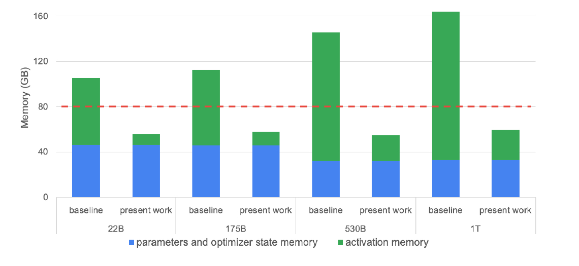
Source: Reducing Activation Recomputation in Large Transformer Models, Figure 1. The dashed line is the paper’s 80 GB device capacity. The bars use the paper’s model and parallelism assumptions.

Rights note: reproduced for technical commentary; rights remain with the authors or publisher. The image is source-reported evidence, not a local measurement.

Generic selective activation checkpointing and this paper’s selective region are related but not identical contracts. A framework policy may save expensive matrix-multiply results while preferring to recompute cheap pointwise operators; the Korthikanti policy specifically removes the quadratic core-attention saved state. Name the policy, region, framework version, and operator set.

0x04H Implementation Traces

Region checkpointing and randomness

PyTorch describes activation checkpointing as retaining function inputs and rerunning the function during backward instead of retaining its internal saved tensors. Current documentation recommends declaring use_reentrant explicitly. A representative non-reentrant path is:

def forward_block(x, block, checkpoint_policy):
    if checkpoint_policy == "full_block":
        return checkpoint(
            block,
            x,
            use_reentrant=False,
            preserve_rng_state=True,
        )
    return block(x)

Dropout makes RNG state part of correctness. PyTorch checkpointing stashes and restores RNG state by default, with runtime overhead. Moving tensors to a new, previously unseen device inside the checkpointed function is outside that determinism guarantee. Stateful updates, mutation, global counters, and data-dependent control flow must also be audited before assuming rerun parity.

Observe what autograd saves

Saved-tensor hooks can inventory the actual forward objects requested by autograd. The hook must record metadata without retaining an extra reference to the original tensor:

def storage_key(t):
    return (t.device, t.untyped_storage().data_ptr(), t.untyped_storage().nbytes())


saved = {}


def pack_hook(t):
    key = storage_key(t)
    saved.setdefault(key, record(
        shape=tuple(t.shape),
        stride=tuple(t.stride()),
        dtype=t.dtype,
        device=t.device,
        storage_bytes=t.untyped_storage().nbytes(),
    ))
    return t


def unpack_hook(t):
    return t


with torch.autograd.graph.saved_tensors_hooks(pack_hook, unpack_hook):
    loss = model(batch).loss
loss.backward()

This inventories unique saved storages for that path. It is not a complete peak trace: it omits unsaved forward temporaries, workspace, gradients created later, allocator rounding, and external allocations. Hooks can also alter behavior if their pack/unpack functions move or transform values.

Reconstruct the liveness cut

An event-based simulator should release before allocating at the same declared event when intervals are half-open:

def peak_from_intervals(objects):
    events = []
    for obj in objects:
        events.append((obj.birth, 1, +obj.unique_storage_bytes, obj.name))
        events.append((obj.death, 0, -obj.unique_storage_bytes, obj.name))

    live = 0
    peak = 0
    peak_event = None
    for event, release_first, delta, name in sorted(events):
        live += delta
        if live > peak:
            peak = live
            peak_event = (event, name)
    return peak, peak_event

For asynchronous streams, a host-side program order is insufficient. The death event must represent completed device use, not merely the Python statement that dropped the final reference.

Measure the allocator boundary

warmup_steps(model, optimizer, batches=3)
torch.cuda.synchronize()
torch.cuda.reset_peak_memory_stats()
torch.cuda.memory._record_memory_history(max_entries=100_000)

run_one_measured_training_step(model, optimizer, batch)
torch.cuda.synchronize()

evidence = {
    "peak_allocated": torch.cuda.max_memory_allocated(),
    "peak_reserved": torch.cuda.max_memory_reserved(),
    "device_used": torch.cuda.device_memory_used(),
}
torch.cuda.memory._dump_snapshot("m4-1-activation-step.pickle")

The underscore-prefixed history APIs are version-sensitive debugging tools. Record the PyTorch/CUDA version, allocator backend, model commit, operator backend, checkpoint policy, microbatch, sequence lengths, and warmup procedure. device_used - reserved is not automatically “NCCL memory”; it is an unattributed residual that needs further evidence.

0x04I Policy Selection Is A Constrained Optimization

For candidate region r, let S_r be saved bytes removed from the peak, F_r additional recomputation work, and Q_r additional transfer bytes. A policy chooses regions under a memory budget:

$$\begin{aligned} \text{minimize}\quad &\sum_r x_r(\lambda_FF_r+\lambda_QQ_r)\\ \text{subject to}\quad &M_{\text{peak}}(x)\leq M_{\text{budget}},\\ &x_r\in\{0,1\}. \end{aligned}$$

This is a design model, not PyTorch’s implementation. It explains why “turn on checkpointing” is incomplete. Good candidates remove bytes that cross the peak cut while adding little work or movement. Recomputing an object that dies before the peak saves no peak memory. Offloading an object after the peak is similarly irrelevant to that peak.

The execution gate is:

same loss and gradients within the declared numerical tolerance
same dropout/randomness contract
lower measured peak at the intended microbatch and sequence distribution
acceptable step-time and communication change
no hidden increase in host memory or external device allocation

0x04J Activation Failure Lab And Publish Gate

Failure	Hidden mistake	Consequence
sum every tensor ever produced	lifetimes ignored	analytical peak overcounted
count tensor views independently	storage aliasing ignored	payload double-counted
call every forward output an activation	backward dependency not inspected	wrong saved-state inventory
treat 34bsh+5bas^2 as Llama memory	MHA, GeLU, dropout, dtype, and operator assumptions replaced	coefficient attached to wrong model
halve the formula because GQA has fewer K/V heads	quadratic query-head state and implementation expansion ignored	savings overclaimed
read saved-tensor hooks as a peak profiler	temporaries, gradients, workspace, and allocator state omitted	measured peak undercounted
add category maxima	maxima occur at different events	process peak overcounted
equate allocated with reserved	caching allocator state ignored	capacity mismatch unexplained
equate snapshot bytes with device use	external allocations invisible	residual assigned to wrong owner
checkpoint stochastic code without RNG contract	replay differs from original forward	wrong gradients
call selective recomputation full checkpointing	region and added work differ	paper/runtime comparison invalid
ignore recomputation and transfer	only memory objective reported	throughput regression hidden
divide by tensor-parallel degree here	global liveness mixed with ownership	parallel section bypassed

Publish gate:

every saved object names the backward formula that needs it
unique storages, not tensor handles, are counted
every object has birth, last use, release, dtype, placement, and byte payload
peak is a maximum cut through simultaneous liveness
workspace, allocated, reserved, and external memory remain separate ledgers
the A16 34 and 5 coefficients are reconstructed from named objects
the running 97/17/1 GiB comparison is labeled as an A16-policy projection
no/selective/full/offload policies expose added work, transfer, and RNG state
saved-tensor inspection and allocator snapshots state their visibility limits
parallel ownership and tiled-attention internals remain explicit handoffs

That is the bridge to M4.2 and M4.3. M4.2 explains where workspace and live tiles reside in the hardware hierarchy. M4.3 shows how an exact tiled attention forward/backward avoids globally materializing the paper’s quadratic objects while reconstructing compact row state inside a custom schedule.

0x05 Forward FLOPs From Tensor Contractions

Parameter counting followed stored tensor axes. Forward-compute accounting now follows executed contractions over those tensors. The same weight can be used once, once per token row, or not at all in a particular phase. Conversely, attention performs arithmetic over query-key pairs that are not learned parameters. A forward ledger therefore cannot be obtained by quoting parameter count alone.

The local owner question is:

Given the immutable architecture and workload records, which scalar contractions does one forward path request, and which parts of that request are mathematical, backend-dependent, or outside the matmul convention?

The answer has four accounting boundaries:

matmul FLOPs:
    multiply/add operations implied by declared tensor contractions

non-matmul primitives:
    reductions, exponentials, reciprocal square roots, rotations,
    comparisons, masks, residual adds, and elementwise nonlinearities

scheduled kernel work:
    operations the selected backend actually issues after tiling,
    padding, fusion, sparsity, and causal specialization

observed runtime:
    elapsed time and hardware counters under one saved environment

This section derives the first boundary, inventories the second, and marks where the third can differ. M4.2 owns the hardware execution and profiler interpretation.

0x05A From One Dot Product To 2MNK

For one output scalar of a matrix product,

$$C_{ij}=\sum_{k=1}^{K}A_{ik}B_{kj},$$

the mathematical expression contains K multiplications and K-1 additions when reduced from scratch. Hardware and analytical literature normally report the operation as K fused multiply-adds. Under this article’s immutable operation convention, one fused multiply-add counts as two FLOPs:

$$F_{\text{dot}} \approx 2K.$$

An [M,K] @ [K,N] product has MN output dots, so:

$$F_{\text{GEMM}}=2MNK.$$

NVIDIA’s matrix-multiplication guide uses the same convention: MNK fused multiply-adds, with each FMA counted as one multiply plus one add. This is a reporting convention, not a statement that an FMA instruction takes two clock cycles. The exact-from-zero scalar count MN(2K-1) and the conventional 2MNK count differ by one addition per output. The conventional form is used throughout because it composes cleanly and matches common throughput reporting.

Bias addition, a nonzero GEMM beta*C term, activation fusion, and epilogues are not silently included:

X: [R, K]
W: [K, N]
Y = X @ W: [R, N]

matmul ledger:        2 * R * K * N FLOPs
optional bias ledger: R * N additions
activation ledger:    separate primitive count

The distinction between MACs and FLOPs must remain visible:

$$1\ \text{MAC}=1\ \text{multiply}+1\ \text{accumulate} \approx 2\ \text{FLOPs}$$

under this convention. A source reporting MACs and another reporting FLOPs can therefore differ by almost exactly two while describing the same contractions.

0x05B Flatten Rows, Preserve Semantic Axes

A linear layer can flatten independent batch/token rows into R=B S_{\text{rows}}:

$$X\in\mathbb{R}^{B\times S_{\text{rows}}\times d_{in}} \longrightarrow X_{\text{flat}}\in\mathbb{R}^{R\times d_{in}}.$$

For W\in\mathbb{R}^{d_{in}\times d_{out}}:

$$F_{\text{linear}} =2R d_{in}d_{out} =2B S_{\text{rows}}d_{in}d_{out}.$$

Flattening is an accounting convenience. It does not erase which rows exist. The running workload records make three different row choices:

Phase	Newly projected rows	Query rows	Visible K/V rows	Default logit rows in this article
full-sequence training	S	S	S	S
prompt prefill	S	S	S	1
one-token decode call	1	1	T	1

Training and prefill have the same block-level contraction shapes in the baseline, but not the same saved state or output policy. Decode projects one new Q/K/V row, attends over T visible K/V rows, and produces one decision row. The detailed phase tables remain in 0x09 and 0x0C; here the row axes are kept explicit so no full-sequence formula is reused by accident.

The A16 source uses the following figure to locate the contractions in a classic dense-MHA, two-matrix-GeLU block:

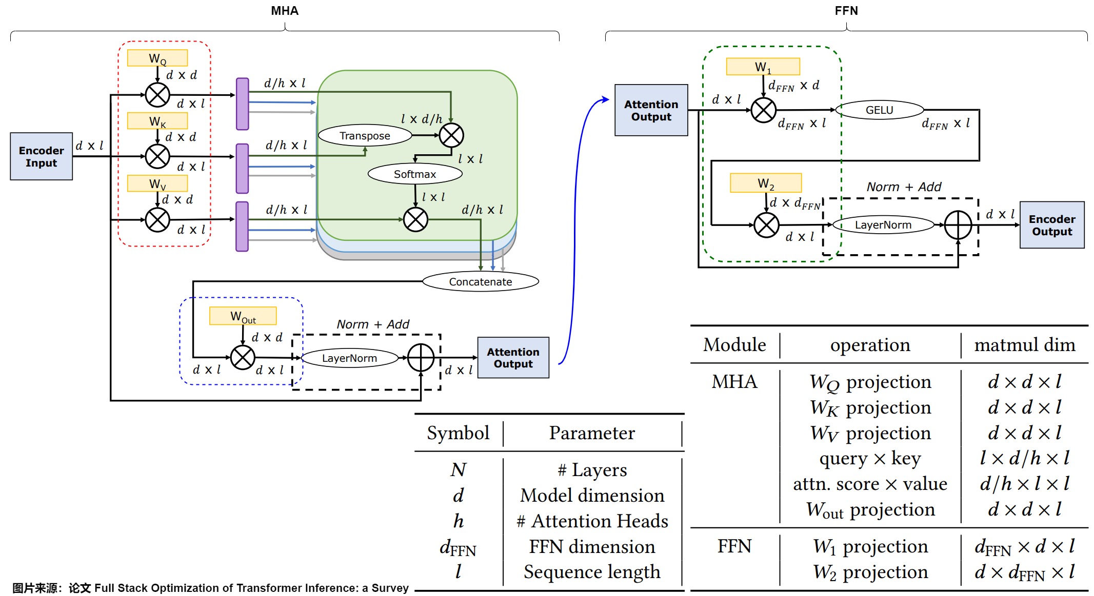
Source figure: Kim et al., Full Stack Optimization of Transformer Inference: a Survey, Figure 1 and Table 2, combined in A16. Reproduced for technical commentary; rights remain with the authors or publisher. M4.1 uses it only for the classic MHA/two-matrix-FFN contraction contract.

The figure originates from Full Stack Optimization of Transformer Inference: a Survey. Its semantic job here is limited: it shows which dimensions meet at each matmul. The running manifest differs in two material ways:

A16/source figure:
    H_q = H_kv
    two FFN projections with GeLU

running fixture:
    H_q = 32, H_kv = 8
    three SwiGLU projections

The formulas below are therefore regenerated from the manifest, not copied from the diagram’s coefficients.

0x05C Q, K, V, And O Projection Contractions

The running GQA block declares:

X_q:   [B, S_q,   d]
X_kv:  [B, S_new, d]

W_Q:   [d,    d_q ]    Q: [B, H_q,  S_q,   d_h]
W_K:   [d,    d_kv]    K: [B, H_kv, S_new, d_h]
W_V:   [d,    d_kv]    V: [B, H_kv, S_new, d_h]
W_O:   [d_q,  d   ]    O: [B, S_q,   d]

For decoder self-attention, S_q=S_new for the newly supplied rows. K/V can later be concatenated with cached rows, but old rows are not reprojected during ordinary decode. Applying 2MNK to each projection gives:

$$\begin{aligned} F_Q &= 2B S_q d d_q,\\ F_K &= 2B S_{new} d d_{kv},\\ F_V &= 2B S_{new} d d_{kv},\\ F_O &= 2B S_q d_q d. \end{aligned}$$

Therefore:

$$F_{\text{attn projections}} =2B\left( S_qdd_q +2S_{new}dd_{kv} +S_qd_qd \right).$$

For training/prefill, S_q=S_{new}=S, so the expression becomes:

$$F_{\text{attn projections}} =2BS\underbrace{\left( dd_q+2dd_{kv}+d_qd \right)}_{P_{\text{attn matrices}}}.$$

This equality is useful but conditional: each projection weight is applied once per row, biases are disabled, and the operation is dense. It explains why a linear stack often contributes approximately two FLOPs per used weight per token without turning 2NP into a universal model formula.

For the running manifest:

d_q  = 4096
d_kv = 1024

P_attn_matrices
  = 4096*4096
  + 2*(4096*1024)
  + 4096*4096
  = 41,943,040 scalars

projection FLOPs/layer
  = 2 * 1 * 4096 * 41,943,040
  = 343,597,383,680
  = 343.597 GFLOPs

Classic MHA would set d_{kv}=d_q=d and recover four square matrices:

$$F_{\text{MHA projections}}=8BSd^2.$$

The running GQA ratio d_{kv}/d=1/4 instead gives:

$$F_{\text{GQA projections}} =4BSd^2+4BSd(d/4) =5BSd^2.$$

GQA therefore reduces K/V projection work and cache width. It does not reduce the number of query heads in the score path.

0x05D QK And PV: Query Heads Own The Pairwise Work

After projection and head layout:

Q: [B, H_q,  S_q, d_h]
K: [B, H_kv, S_k, d_h]
V: [B, H_kv, S_k, d_h]

Each query head maps to one K/V group. A semantic repeat or grouped kernel makes the selected K/V head available to its query heads without changing the logical score output:

Q @ K^T -> scores: [B, H_q, S_q, S_k]
P @ V   -> heads:  [B, H_q, S_q, d_h]

For every one of B H_q S_q S_k score entries, QK^T contracts d_h channels:

$$F_{QK^\top}=2B H_q S_q S_k d_h.$$

For every one of B H_q S_q d_h output entries, PV reduces over S_k:

$$F_{PV}=2B H_q S_q S_k d_h.$$

Together:

$$F_{\text{attention matmuls}} =4B H_qS_qS_kd_h =4B S_qS_kd_q.$$

At fixed H_q and d_h, lowering H_{kv} does not lower this ideal pairwise count. It changes K/V projection width, stored K/V state, broadcast or grouping behavior, and kernel layout. M3.2 owns those local head semantics; M4.1 prices the resulting axes.

For running full-row attention:

QK^T FLOPs/layer
  = 2 * 1 * 32 * 4096 * 4096 * 128
  = 137,438,953,472
  = 137.439 GFLOPs

P @ V FLOPs/layer
  = 137,438,953,472
  = 137.439 GFLOPs

pairwise matmul total/layer
  = 274,877,906,944
  = 274.878 GFLOPs

Causal legality is not a universal kernel discount

For one unpadded full-sequence causal example, the number of legal query-key pairs per head is triangular:

$$N_{\text{legal pairs/head}} =\sum_{i=1}^{S}i =\frac{S(S+1)}{2}.$$

If an implementation executes only those legal dots, useful mathematical work for both pairwise matmuls is:

$$F_{\text{causal,useful}} =4B H_q d_h\frac{S(S+1)}{2} =2B H_qS(S+1)d_h.$$

Relative to the rectangular 4BH_qS^2d_h ledger:

$$\frac{F_{\text{causal,useful}}}{F_{\text{rectangular}}} =\frac{S+1}{2S}.$$

At S=4096 that ratio is 0.500122, not exactly one half because the diagonal is legal. The corresponding useful pairwise work is 137,472,507,904 FLOPs rather than 274,877,906,944 rectangular FLOPs.

That calculation does not prove that every causal implementation executes half the arithmetic:

Ledger	What it answers	Causal treatment
legal mathematical pairs	Which dependencies may affect the exact result?	triangular
algorithm-scheduled tiles	Which score/value tiles does the backend request?	backend-specific; diagonal and boundary tiles may be padded
issued hardware work	Which instructions were executed?	kernel, dtype, sparsity, and hardware-specific
profiler estimate	Which supported operators received formula estimates?	tool-specific and potentially rectangular

A dense GEMM followed by masking can execute the full rectangle. A causal-aware tiled kernel can skip upper-triangular tiles while still performing extra work inside diagonal or padded tiles. Ragged batches add another boundary:

$$N_{\text{legal,batch}} =H_q\sum_{i=1}^{B}\frac{S_i(S_i+1)}{2},$$

while a padded rectangular schedule may be shaped by BH_qS_{\max}^2. A single remembered “divide attention by two” rule cannot represent all four ledgers.

0x05E SwiGLU: Three Projections, Not A Renamed Two-Layer FFN

The running MLP receives X\in\mathbb{R}^{B\times S\times d} and declares:

gate = X @ W_gate: [B,S,d_ff]
up   = X @ W_up:   [B,S,d_ff]
mixed = SiLU(gate) * up
Y = mixed @ W_down: [B,S,d]

The three matmuls are:

$$\begin{aligned} F_{\text{gate}} &= 2BSdd_{ff},\\ F_{\text{up}} &= 2BSdd_{ff},\\ F_{\text{down}} &= 2BSd_{ff}d. \end{aligned}$$

Thus:

$$F_{\text{SwiGLU matmuls}}=6BSdd_{ff}.$$

The SiLU evaluation and gated elementwise product are real work, but they are not matrix contractions and stay in the non-matmul ledger.

For d_{ff}=14336=3.5d:

$$F_{\text{SwiGLU matmuls}} =21BSd^2.$$

Running value:

6 * 1 * 4096 * 4096 * 14336
  = 1,443,109,011,456
  = 1.443109 TFLOPs/layer

A16’s classic teaching block uses a two-matrix FFN with d_{ff}=4d:

up:   [BS,d] @ [d,4d]  -> [BS,4d]   = 8BSd^2 FLOPs
down: [BS,4d] @ [4d,d] -> [BS,d]    = 8BSd^2 FLOPs

classic FFN total = 16BSd^2 FLOPs

These designs should be compared by their actual projection count and intermediate width, not by applying the phrase “approximately 4d” to both. M3.6 derives why gated variants often adjust d_{ff} to keep a comparable parameter/compute budget.

0x05F Reconstruct A16, Then Reconcile The Running Block

The classic A16 dense-MHA, 4d two-matrix FFN case adds:

Component	Derivation	FLOPs
Q/K/V projections	three [BS,d]@[d,d]	6BSd^2
O projection	one [BS,d]@[d,d]	2BSd^2
two-matrix FFN	d -> 4d -> d	16BSd^2
QK	[B,H,S,d_h]@[B,H,d_h,S]	2BS^2d
PV	[B,H,S,S]@[B,H,S,d_h]	2BS^2d

Therefore:

$$F_{\text{A16 classic block}} =24BSd^2+4BS^2d.$$

The formula is correct for its stated architecture and rectangular operation convention. Its coefficients are not properties of the word “Transformer.”

The running GQA/SwiGLU fixture has:

GQA projections: 5BSd^2
SwiGLU matmuls: 21BSd^2
QK + PV:         4BS^2d

so:

$$F_{\text{running block}} =26BSd^2+4BS^2d.$$

The GQA projection term is lower than classic MHA, but the chosen three-projection SwiGLU width makes the total linear coefficient larger:

Architecture case	Attention projections	MLP projections	Pairwise attention	Block total
A16 dense MHA + 4d GeLU FFN	8BSd^2	16BSd^2	4BS^2d	24BSd^2+4BS^2d
running GQA + 3.5d SwiGLU	5BSd^2	21BSd^2	4BS^2d	26BSd^2+4BS^2d

For B=1,S=d=4096:

A16 classic block:
    24*B*S*d^2 + 4*B*S^2*d
  = 1,924,145,348,608 FLOPs
  = 1.924145 TFLOPs

running GQA/SwiGLU block:
    26*B*S*d^2 + 4*B*S^2*d
  = 2,061,584,302,080 FLOPs
  = 2.061584 TFLOPs

The difference is not evidence that GQA failed to save work. It is evidence that two architectural changes moved different terms in opposite directions.

0x05G Vocabulary Projection: Choose Rows Before Counting

Embedding input is a table lookup:

token_ids: [B,S]
E:         [V,d]
X = E[token_ids]: [B,S,d]

The lookup reads selected rows; it is not a dense [B,S,V]@[V,d] multiplication. The output head is different:

H_selected: [R_logits,d]
W_vocab^T:  [d,V]
logits:     [R_logits,V]

Therefore:

$$F_{\text{logits}}=2R_{\text{logits}}dV.$$

The correct R_{\text{logits}} comes from the execution contract:

Output contract	R_{\text{logits}}	Matmul FLOPs
all supervised training rows	BS	2BSdV
final valid row per prefill request	B	2BdV
one-token decode decision	B	2BdV
API returns all prompt logits	BS	2BSdV

For the running fixture:

one final-row projection
  = 2 * 1 * 4096 * 128256
  = 1,050,673,152 FLOPs
  = 1.050673 GFLOPs

all 4096 rows
  = 2 * 1 * 4096 * 4096 * 128256
  = 4,303,557,230,592 FLOPs
  = 4.303557 TFLOPs

Weight tying does not make the output projection free. It makes embedding lookup and output projection reference the same storage. The forward operations remain different. A fused linear-cross-entropy kernel can avoid materializing all logits in HBM, but it still performs the declared vocabulary contractions unless it implements an independently justified approximation.

0x05H Non-Matmul Work Is A Typed Ledger, Not Zero

The matrix terms dominate many large training and prefill cases, but “omitted from the GEMM formula” does not mean “free.” Nonlinear and reduction primitives do not have one portable FLOP conversion. An exponential, reciprocal square root, comparison, random-number generation, and scalar addition have different hardware paths and profiler treatment.

M4.1 therefore records primitive families and extents:

Primitive family	Logical extent	Required work	Why no universal scalar-FLOP coefficient
RMSNorm	B S d per norm	square, width reduction, epsilon, reciprocal square root, scale	reduction tree, precision, and fusion differ
RoPE	Q and newly projected K coordinates	paired rotations using sin/cos tables or equivalent formulation	precomputed tables, complex kernels, and fusion differ
score scaling	B H_qS_qS_k scores	multiply by 1/\sqrt{d_h}	may fuse into Q, GEMM alpha, or softmax
causal/padding mask	score domain	compare/select or additive bias	boolean, additive, interval, or implicit causal paths differ
softmax	each legal/materialized score row	max, subtract, exp, sum, divide	exp and reductions are not portable one-FLOP operations
SiLU and gate	B S d_{ff}	sigmoid/exp path plus multiplies	approximation and fused epilogue differ
residual update	B S d per branch	elementwise add	may fuse with projection/norm
dropout when enabled	affected tensor extent	RNG, compare, mask/scale multiply	training-only policy and RNG backend differ
vocabulary loss	R_{\text{logits}}V domain	log-sum-exp, target selection, reduction	may fuse with sharded or tiled projection

A useful report can state:

matmul FLOPs:
    exact under the declared FMA convention and contraction shapes

primitive counts:
    N_exp, N_rsqrt, N_compare, N_rng, N_elementwise, reduction extents

backend work:
    measured or inspected separately

PyTorch’s torch.profiler(..., with_flops=True) documentation is deliberately narrow: it uses formulas to estimate FLOPs for specific operators, currently matrix multiplication and 2D convolution. A profiler table that contains a flops column is therefore not automatically a complete model operation count. Missing softmax or normalization FLOPs are a tool-scope issue, not proof that those operators performed no work.

0x05I Complete Running Forward Ledger

The block-level rectangular matmul ledger is:

Component	Exact FLOPs/layer	Decimal unit	Share of block matmul FLOPs
Q/K/V/O projections	343,597,383,680	343.597 GFLOPs	16.667%
QK^T	137,438,953,472	137.439 GFLOPs	6.667%
P@V	137,438,953,472	137.439 GFLOPs	6.667%
SwiGLU projections	1,443,109,011,456	1.443109 TFLOPs	70.000%
one decoder block	2,061,584,302,080	2.061584 TFLOPs	100%

Across L=32 blocks:

$$F_{\text{block stack}} =32(2{,}061{,}584{,}302{,}080) =65{,}970{,}697{,}666{,}560.$$

32-block stack exact
  = 65,970,697,666,560 FLOPs
  = 65.970698 TFLOPs

Adding the phase-specific output head gives:

Forward boundary	Block stack	Logit projection	Total matmul FLOPs
prefill with final-row logits	65.970698 TFLOPs	0.001051 TFLOPs	65.971748 TFLOPs
full training rows before backward	65.970698 TFLOPs	4.303557 TFLOPs	70.274255 TFLOPs

These totals include:

32 decoder-block matrix contractions
the declared vocabulary projection rows
the FMA=2 reporting convention
rectangular QK/PV contractions

They exclude:

embedding row-gather work
RMSNorm, RoPE, masks, softmax, SiLU, gates, residuals, and loss primitives
padding, tile-rounding, or causal kernel savings/overwork
communication and data movement
backward, recomputation, gradient reduction, and optimizer work

The last line is a hard boundary. Backward and recomputation require their own dX, dW, and schedule ledger rather than multiplying this forward number by an unexplained constant.

0x05J Executable Formula Trace And Assertions

A cost estimator should emit named contractions, not only one total:

def gemm_flops(m, k, n, batch=1):
    assert min(m, k, n, batch) >= 0
    return 2 * batch * m * k * n


def forward_matmul_ledger(arch, work, logits_rows):
    d = arch.hidden_size
    dq = arch.num_attention_heads * arch.head_dim
    dkv = arch.num_key_value_heads * arch.head_dim
    dff = arch.intermediate_size

    assert dq == d, "running fixture expects packed query width == residual width"
    assert work.query_length == work.new_input_length
    assert work.key_value_length >= work.new_input_length

    B = work.batch_size
    Sq = work.query_length
    Snew = work.new_input_length
    Sk = work.key_value_length
    Hq = arch.num_attention_heads
    dh = arch.head_dim

    ops = [
        ("q_proj", gemm_flops(B * Sq,   d,   dq)),
        ("k_proj", gemm_flops(B * Snew, d,   dkv)),
        ("v_proj", gemm_flops(B * Snew, d,   dkv)),
        ("qk",     gemm_flops(Sq, dh, Sk, batch=B * Hq)),
        ("pv",     gemm_flops(Sq, Sk, dh, batch=B * Hq)),
        ("o_proj", gemm_flops(B * Sq,   dq,  d)),
        ("gate",   gemm_flops(B * Snew, d,   dff)),
        ("up",     gemm_flops(B * Snew, d,   dff)),
        ("down",   gemm_flops(B * Snew, dff, d)),
    ]

    logits = ("logits", gemm_flops(logits_rows, d, arch.vocab_size))
    return ops, logits

The tensor axes make two implementation errors visible:

1. k_proj and v_proj use S_new, not the complete cached S_k, in ordinary cached decode.
2. qk and pv use H_q because each query head computes an output even when several query heads share one K/V head.

Mechanical tests for the running full-row fixture:

ops, logits = forward_matmul_ledger(
    arch=running_manifest,
    work=train_full_4k,
    logits_rows=1 * 4096,
)

by_name = dict(ops)

assert by_name["q_proj"] + by_name["k_proj"] \
     + by_name["v_proj"] + by_name["o_proj"] \
     == 343_597_383_680

assert by_name["qk"] == 137_438_953_472
assert by_name["pv"] == 137_438_953_472

assert by_name["gate"] + by_name["up"] + by_name["down"] \
     == 1_443_109_011_456

assert sum(value for _, value in ops) == 2_061_584_302_080
assert logits[1] == 4_303_557_230_592

The A16 coefficient can also be tested as an architecture case:

classic_linear = 8 * B * S * d**2 + 16 * B * S * d**2
classic_pairs  = 4 * B * S**2 * d

assert classic_linear + classic_pairs \
     == 24 * B * S * d**2 + 4 * B * S**2 * d

Profiler reconciliation must retain the same scope:

with torch.profiler.profile(
    activities=[ProfilerActivity.CPU, ProfilerActivity.CUDA],
    record_shapes=True,
    with_flops=True,
) as prof:
    model(inputs)

# Compare supported matmul operator estimates with named contractions.
# Do not treat the sum as a complete non-matmul or hardware-issued count.

A mismatch is a diagnosis prompt:

shape mismatch:
    wrong rows, widths, head mapping, or vocabulary policy

operator mismatch:
    fused, decomposed, recomputed, skipped, or unsupported profiler op

backend-work mismatch:
    causal/tile padding, sparsity, quantization, or implementation schedule

observation mismatch:
    stale model revision, warmup, asynchronous timing, or incomplete capture

Do not silently tune the formula until it matches one profiler total. First identify which accounting boundary differs.

0x05K Failure Lab And Publish Gate

Failure	Misleading result	Repair
report MACs as FLOPs	values are about 2x too small	publish the FMA/MAC convention
reuse four square MHA projections for GQA	K/V projection work is overstated	derive d_q and d_{kv} from head counts
use H_{kv} in QK/PV	pairwise work is understated	count query-head outputs with H_q
halve every causal attention number	backend work is asserted without a kernel contract	separate legal pairs, scheduled tiles, and observed work
project all prompt rows for a final-row API	vocabulary work and logits storage are overstated	bind R_{\text{logits}} to output policy
treat tied embeddings as free logits	storage sharing is confused with execution	count lookup and projection separately
omit softmax/norm because profiler reports no FLOPs	tool support is mistaken for zero work	keep a typed non-matmul primitive ledger
add backward as an unexplained multiplier	training policy is hidden	derive dX, dW, recomputation, and optimizer terms separately
read analytical FLOPs as latency	movement, occupancy, fusion, and launch costs disappear	hand execution to M4.2 and traffic to 0x08

Publish gate:

2MNK is derived from MN output dot products under FMA=2
every decoder-block matmul names its input, contraction, and output axes
GQA projection savings are not applied to query-head pairwise work
A16's 24/4 coefficients remain attached to dense MHA plus a 4d two-matrix FFN
the running 26/4 coefficients are reconstructed from GQA plus 3.5d SwiGLU
causal legal pairs are separate from backend-scheduled and profiler work
all-row and final-row logits are separate execution contracts
non-matmul primitives remain visible without invented universal coefficients
the complete running forward ledger passes exact integer assertions
backward, recomputation, optimizer, communication, and runtime remain explicit handoffs

0x06 Backward, Recomputation, And Training-Compute Conventions

The forward ledger is only one side of training. Reverse-mode automatic differentiation traverses the graph in the opposite direction, consumes saved or reconstructed state, produces gradients for activations and trainable weights, and eventually hands those gradients to an optimizer and a distributed schedule. Calling all of that “backward is twice forward” hides both the reason the approximation often works and the cases where it does not.

The local owner question is:

Starting from the exact forward contractions in 0x05, which backward contractions are required, which forward regions are replayed, and which training costs must remain outside the familiar 3x and 6ND shorthand?

The answer is a sum of named ledgers:

$$F_{train} =F_{forward}+F_{backward}+F_{recompute}+F_{optimizer}+F_{other}.$$

Communication is recorded beside this arithmetic sum, not silently converted into model FLOPs:

$$Q_{communication} =Q_{gradient\ collective}+Q_{parameter\ collective}+Q_{pipeline}.$$

The distinction matters because a gradient all-reduce can dominate elapsed time without changing the model’s mathematical forward/backward FLOP count. Section 0x07 derives per-rank state and collective payloads; M4.2 owns overlap, achieved throughput, and hardware counters.

0x06A Derive The Two Backward Matrix Products

Consider the same bias-free linear map used in 0x05:

$$X\in\mathbb{R}^{M\times K},\qquad W\in\mathbb{R}^{K\times N},\qquad Y=XW\in\mathbb{R}^{M\times N}.$$

Let $G=\partial\mathcal{L}/\partial Y$ be the upstream gradient. One output entry is

$$Y_{mn}=\sum_{k=1}^{K}X_{mk}W_{kn}.$$

For an input entry $X_{mk}$, the chain rule accumulates contributions from all output columns $n$:

$$\frac{\partial\mathcal{L}}{\partial X_{mk}} =\sum_{n=1}^{N} \frac{\partial\mathcal{L}}{\partial Y_{mn}} \frac{\partial Y_{mn}}{\partial X_{mk}} =\sum_{n=1}^{N}G_{mn}W_{kn}.$$

That scalar equation is the matrix product

$$dX=GW^T,$$

with shapes [M,N] @ [N,K] -> [M,K] and conventional cost

$$F_{dX}=2MNK.$$

For one weight entry $W_{kn}$, every input row contributes:

$$\frac{\partial\mathcal{L}}{\partial W_{kn}} =\sum_{m=1}^{M} \frac{\partial\mathcal{L}}{\partial Y_{mn}} \frac{\partial Y_{mn}}{\partial W_{kn}} =\sum_{m=1}^{M}X_{mk}G_{mn}.$$

Therefore

$$dW=X^TG,$$

with shapes [K,M] @ [M,N] -> [K,N] and

$$F_{dW}=2KMN=2MNK.$$

The three dense matrix products have equal leading-order work:

Path	Contraction	Output	Matmul FLOPs
forward	X[M,K] @ W[K,N]	Y[M,N]	$2MNK$
input gradient	G[M,N] @ W.T[N,K]	dX[M,K]	$2MNK$
weight gradient	X.T[K,M] @ G[M,N]	dW[K,N]	$2MNK$

An optional bias has a different backward shape:

$$db_n=\sum_{m=1}^{M}G_{mn}.$$

That is a reduction over rows, not another 2MNK GEMM. It belongs in the non-matmul primitive ledger. The same rule applies to activation derivatives, normalization backward, softmax backward, dropout masks, residual accumulation, loss gradients, and gradient clipping: they are real work, but the linear-layer derivation does not manufacture a universal coefficient for them.

0x06B Why The Ideal Dense Path Is 3x Forward

For a trainable dense matrix used once over the same $M$ rows,

$$F_{backward,matmul}=F_{dX}+F_{dW}=4MNK=2F_{forward,matmul},$$

so forward plus backward is

$$F_{fwd+bwd,matmul}=6MNK=3F_{forward,matmul}.$$

The 3x is not an empirical performance constant. It is a contraction count under a precise graph contract:

the forward operation is a dense matrix product
both the input gradient and weight gradient are required
the same logical row extent is used by all three contractions
one multiply plus one add is reported as two FLOPs
recomputation, optimizer, collectives, and non-matmul primitives are excluded

Change the graph and the multiplier can change:

Design choice	Required contraction change	Consequence
frozen weight, trainable upstream path	omit dW; retain dX	local dense path is about 2x forward, not 3x
no gradient needed for the input	omit dX; retain dW	also about 2x forward
frozen weight and stopped input gradient	omit both	forward only
shared/tied weight used at two call sites	accumulate gradient contributions from both uses	unique storage count does not equal use count
sparse/routed operation	backward follows active routes and sparse kernel contract	total parameter count is not active work
custom fused attention backward	recompute and fuse selected primitives	mathematical gradients remain, scheduled work and traffic differ

Gradient accumulation across microbatches does not remove each microbatch’s dW contraction. It changes when gradient buffers are accumulated, reduced, and consumed by the optimizer. Likewise, mixed precision changes operand and accumulation representations; it does not by itself erase a required contraction.

0x06C Attention And The Vocabulary Head Follow The Graph

The two pairwise attention matmuls also have forward and backward contractions. For the score path $S=QK^T$, backward requires products that accumulate $dQ$ and $dK$. For $O=PV$, backward accumulates $dP$ and $dV$. If every operand lies on a trainable path, their leading matmul work again follows the forward plus two-backward pattern. Softmax, scaling, masking, and dropout backward remain separate primitives.

This is especially important for IO-aware attention. A FlashAttention-style backward can reconstruct score and probability tiles from compact row state instead of reading a globally saved $S$ or $P$. That changes the recomputation and traffic ledger, not the derivatives that must ultimately be produced. M4.3 owns that tiled algorithm.

For all-row training logits,

$$H\in\mathbb{R}^{BS\times d},\qquad W_{vocab}\in\mathbb{R}^{d\times V},\qquad Z=HW_{vocab},$$

the matmul ledger is:

$$F_{Z}=2BSdV,\qquad F_{dH}=2BSVd,\qquad F_{dW_{vocab}}=2BSdV.$$

Therefore the trainable untied head contributes $6BSdV$ before the cross-entropy primitives. Tying the input embedding and output head can reduce unique stored parameters, but the output projection still executes and its gradient must be accumulated into the shared weight. The embedding lookup’s backward is an indexed scatter/accumulation; it is not a dense 2BSdV product.

0x06D Recomputation Is A Region Schedule, Not A Universal Fourth Pass

Section 0x04 compared saved-state policies by memory. The compute view names which forward regions are actually replayed. Let $\mathcal{R}$ be the set of recomputed regions and let $F_{forward}(r)$ be the forward work of region $r$:

$$F_{recompute}=\sum_{r\in\mathcal{R}}n_{replay}(r)F_{forward}(r).$$

If an ideal dense matmul graph has forward cost $F$ and a fraction $\rho$ of that same matmul work is replayed once, then

$$F_{train,matmul}=(3+\rho)F, \qquad 0\leq\rho\leq1.$$

This compact form is useful only when $\rho$ is defined over the same forward operation set. The explicit sum is safer because real policies differ:

Policy	Retained/reconstructed boundary	Added arithmetic or transfer
no recomputation	retain declared backward dependencies	no deliberate forward replay
selective core-attention recomputation	discard selected score/probability state	replay QK, softmax/dropout policy, and PV region
full block checkpointing	retain block or segment inputs	replay the checkpointed blocks, not automatically the head/loss
saved-tensor offload	preserve selected values outside device memory	D2H/H2D traffic; not a forward replay policy
custom fused backward	retain compact sufficient state	replay implementation-defined local primitives

PyTorch’s checkpoint contract also warns that replay must be functionally equivalent to the original forward. Global state, device movement, or different randomness can produce wrong gradients. The compute ledger therefore stores region identity, replay count, RNG/mask policy, and operator revision beside the added FLOPs.

0x06E Running-Fixture Training Ledger

The full-row training forward from 0x05 contains:

32-block stack:       65,970,697,666,560 FLOPs
all-row output head:   4,303,557,230,592 FLOPs
forward matmul total: 70,274,254,897,152 FLOPs

Under the ideal trainable-matmul contract, backward is exactly two copies of that forward contraction ledger:

Training path	Forward	Backward	Replay	Matmul total
no recomputation	70.274255 TF	140.548510 TF	0	210.822765 TF
selective QK/PV replay in all 32 blocks	70.274255 TF	140.548510 TF	8.796093 TF	219.618858 TF
replay every block, not the output head	70.274255 TF	140.548510 TF	65.970698 TF	276.793462 TF
replay every counted forward matmul	70.274255 TF	140.548510 TF	70.274255 TF	281.097020 TF

The rounded TFLOP rows above come from these exact integer contracts:

no recomputation:              210,822,764,691,456 FLOPs
selective QK/PV replay:        219,618,857,713,664 FLOPs
replay decoder blocks only:    276,793,462,358,016 FLOPs
replay every counted matmul:   281,097,019,588,608 FLOPs

The selective row counts only the QK and PV matmuls in the core-attention region. Replayed softmax, mask, scale, and dropout primitives remain outside this matmul total. It is not a prediction of one framework’s exact selective checkpoint implementation.

The third and fourth rows expose a common error. Blindly multiplying the whole forward by four adds one unnecessary replay of the vocabulary head:

$$281.097020-276.793462=4.303557\ \text{TFLOPs}.$$

That difference is exactly one head forward, about 1.53% of the blind 4x total. The percentage is fixture-specific; the structural error is general.

These values still exclude non-matmul primitives, optimizer work, communication, input pipeline work, and backend padding or fusion. They are an exact integer reconciliation of the declared matmul ledger, not a measured step-time model.

0x06F Derive 6ND, Then Name Its Parameter Set

Suppose $N_{used}$ counts dense matrix-weight scalars that are each used once per processed token in the declared forward path, and $D_{seen}$ counts token presentations processed by that path. One forward pass performs approximately one multiply and one add per used weight and token:

$$F_{forward}\approx2N_{used}D_{seen}.$$

The two backward contractions add approximately $4N_{used}D_{seen}$:

$$F_{fwd+bwd}\approx6N_{used}D_{seen}.$$

That is the origin of 6ND. It is a useful product proxy, not an identity over the checkpoint’s unique scalar count. Its assumptions are:

N counts the dense matrices actually used by the modeled token path
each counted matrix is used once per token presentation
both dX and dW are required
there is no activation replay term
pairwise attention work is omitted or added separately
embedding lookup, norms, activations, loss, optimizer, and collectives are omitted
weight tying and repeated module use are reconciled by operations, not unique storage
D counts processed token presentations, including repeated data

The running fixture makes the choice of $N$ testable. The block matrix weights plus the untied output head contain

$$N_{used}=6{,}979{,}321{,}856+525{,}336{,}576 =7{,}504{,}658{,}432.$$

For $D_{seen}=4096$ rows:

$$6N_{used}D_{seen}=184{,}434{,}485{,}624{,}832.$$

The omitted QK/PV training matmuls contribute

$$3\times8{,}796{,}093{,}022{,}208 =26{,}388{,}279{,}066{,}624,$$

and the two terms close exactly against the no-recompute matmul ledger:

$$184{,}434{,}485{,}624{,}832 +26{,}388{,}279{,}066{,}624 =210{,}822{,}764{,}691{,}456.$$

Using all 8,030,261,248 unique learned scalars instead gives 197.351700 TF, about 6.4% below the exact matmul ledger. That apparent closeness is not a better derivation: it incorrectly treats the input embedding lookup and norm scales as dense per-token matrices while still omitting pairwise attention. Two errors partly cancel. Using only Kaplan-style non-embedding block matrices gives 171.523814 TF, about 18.6% below this fixture’s exact total because this fixture’s untied large vocabulary head and pairwise work are both material.

Sparse MoE requires active experts per token rather than total expert storage; M6.1 owns that ledger. Dataset uniqueness, repetition, and effective sample size are not encoded by $D_{seen}$; M4.7 owns those empirical consequences.

0x06G Four Paper Contracts That Must Not Be Mixed

A16 reused Kaplan’s table to introduce the relation between parameter count and forward FLOPs. The image remains useful when read as a declared paper contract: its N excludes vocabulary and positional embeddings, its forward total retains a context-dependent attention term, and its later 6N proxy drops that term for the studied width/context regime.

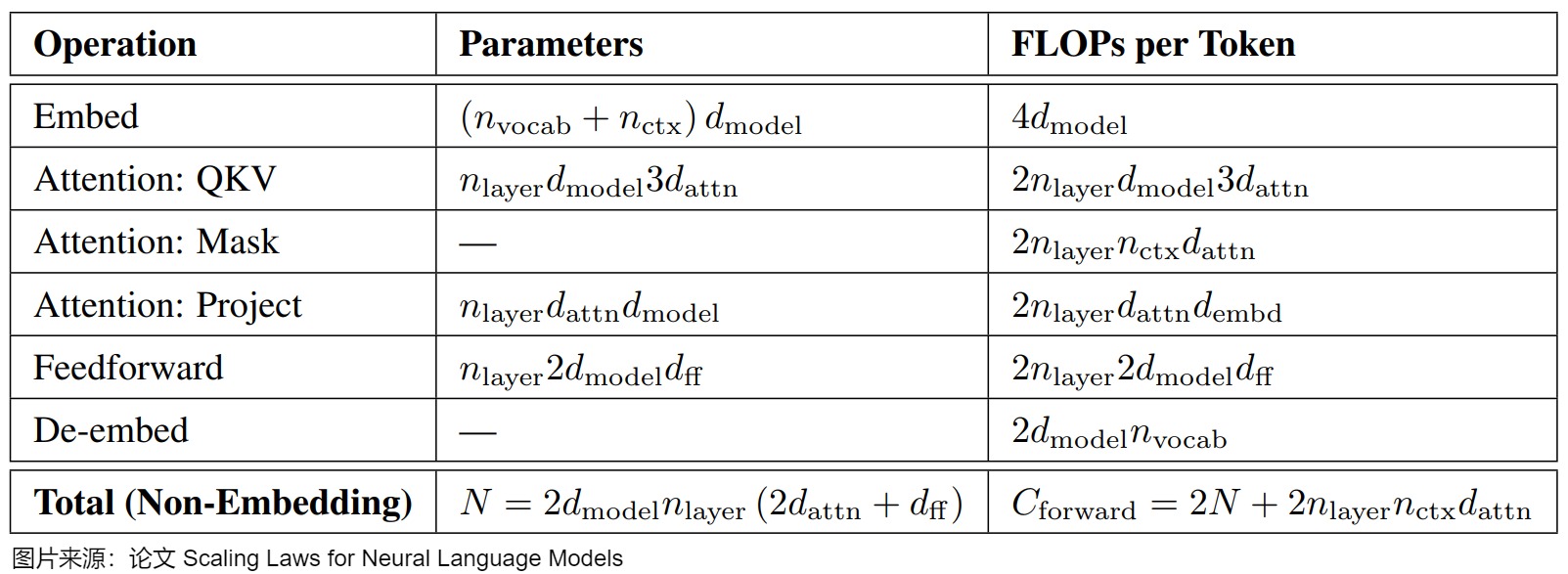
Source figure: Kaplan et al., Scaling Laws for Neural Language Models, Table 1, reproduced in A16. Reproduced for technical commentary; rights remain with the authors or publisher. Its non-embedding N coordinate and omitted-work boundary are preserved below.

Source-local figure from A16, adapted there from Kaplan et al. Table 1. The paper contract, not the image alone, controls the interpretation.

The papers below use related arithmetic but not one interchangeable C:

Source contract	Parameter/work coordinate	Forward/backward convention	Replay and omitted-work boundary
Kaplan et al.	$N$ excludes vocabulary and positional embeddings	$C\approx6NBS$, where processed token presentations map to batch tokens times updates	drops context-dependent attention from the headline proxy; omits subleading primitives
Hoffmann et al. (Chinchilla)	model size includes embedding matrices; detailed FLOPs include embedding, attention, dense block, softmax, and final logits	detailed forward ledger multiplied by three for backward; compared with $6ND$	no separately stated rematerialization term in Appendix F’s formula; exact/proxy ratio is architecture-dependent
Narayanan et al. (Megatron)	architecture-shaped GPT GEMM ledger with $L,h,S,V$	blocks use forward + backward + one replay; head uses forward + backward	Equation 3 is a lower bound over named GEMMs and assumes activation recomputation
Chowdhery et al. (PaLM)	dense non-attention matmul proxy plus a separate dense-attention term	$6N$ non-attention and $12LHQT$ attention FLOPs per token before rematerialization	reports model FLOPs separately from hardware FLOPs including selective rematerialization

Chinchilla Appendix F is an instructive validation rather than a universal proof. It reports detailed-to-6ND ratios from 1.03, 1.10, 1.08, 1.04, 1.03, to 0.99 across six listed model sizes from 73M to 6.8B. The proxy was close over that family; the ratio still moved with architecture.

PaLM makes the replay boundary unusually explicit. Its Appendix B reports that PaLM 540B recomputed 75% of non-attention forward FLOPs and all attention forward FLOPs. The paper lists 3.28 TFLOPs/token before rematerialization and 4.10 TFLOPs/token with rematerialization for that model. Those are source-reported accounting values, not claims about the running fixture.

Correcting The A16 Megatron Transcription

For the classic MHA and two-matrix 4h FFN geometry, Megatron derives the forward block cost from A16’s familiar form:

$$F_{block,fwd}=24BSh^2+4BS^2h.$$

The paper then counts forward + two backward contractions + one block replay:

$$F_{blocks}=4L(24BSh^2+4BS^2h) =96BSLh^2\left(1+\frac{S}{6h}\right).$$

The vocabulary head is not checkpointed in that derivation. It contributes forward plus backward:

$$F_{head}=6BShV.$$

The primary paper’s Equation 3 is therefore

$$F_{Megatron} =96BSLh^2\left(1+\frac{S}{6h}+\frac{V}{16Lh}\right).$$

The $V/(16Lh)$ term already expands to $6BShV$. A16’s displayed training formula appends another +2BShV; that extra term is not present in Megatron Equation 3 and conflicts with A16’s own preceding statement that the head costs 2BShV forward plus 4BShV backward. M4.1 keeps the local source as provenance but uses the primary equation as the corrected contract.

The same distinction explains the running fixture’s 276.793462 TF row: replay the blocks once, count the head three times, and do not replay the head unless the actual checkpoint region includes it.

0x06H Optimizer And Communication Are Separate Terms

AdamW illustrates why optimizer work should not be expressed as another forward multiplier. For each updated scalar, a conceptual step computes:

$$m_t=\beta_1m_{t-1}+(1-\beta_1)g_t,$$ $$v_t=\beta_2v_{t-1}+(1-\beta_2)g_t^2,$$

followed by bias correction, normalization, optional weight decay, and the parameter update. Its work scales approximately as

$$F_{optimizer}=c_{optimizer}P_{updated},$$

but $c_{optimizer}$ is policy- and implementation-specific. Fused/foreach kernels, master weights, loss scaling, clipping, AMSGrad, stochastic rounding, and lower-precision states change the primitive sequence and traffic. The optimizer often has much lower arithmetic intensity than the model GEMMs. The persistent state shapes were derived in 0x03; M4.2 owns the runtime behavior.

Distributed training adds another independent contract:

data parallel:
    gradient reduction or reduce-scatter payload

tensor parallel:
    activation/gradient collectives around sharded contractions

pipeline parallel:
    activation and gradient sends between stages

sharded optimizer/parameters:
    all-gather, reduce-scatter, and transient materialization

Collective reductions execute arithmetic, but paper model-FLOP conventions normally do not include network reduction adds in 6ND. Record at least the logical payload, collective type, participant group, dtype, and replay/overlap schedule. Do not divide the global model FLOPs by world size and call the result per-rank runtime.

0x06I Executable Training-Ledger Trace

The accounting code should preserve region identity and graph requirements:

def linear_training_matmuls(M, K, N, *, need_dx=True, need_dw=True):
    forward = gemm_flops(M, K, N)
    dx = gemm_flops(M, N, K) if need_dx else 0
    dw = gemm_flops(K, M, N) if need_dw else 0

    assert forward == 2 * M * K * N
    if need_dx and need_dw:
        assert dx == forward
        assert dw == forward

    return {"forward": forward, "dX": dx, "dW": dw}


def training_matmul_ledger(forward_regions, replay_counts):
    forward = sum(region.flops for region in forward_regions)
    backward = sum(
        region.dx_flops + region.dw_flops
        for region in forward_regions
    )
    replay = sum(
        replay_counts.get(region.name, 0) * region.flops
        for region in forward_regions
    )
    return {
        "forward": forward,
        "backward": backward,
        "recompute": replay,
        "model_matmul_total": forward + backward + replay,
    }

Running-fixture assertions fail closed:

base = training_matmul_ledger(full_forward_regions, replay_counts={})
assert base["forward"] == 70_274_254_897_152
assert base["backward"] == 140_548_509_794_304
assert base["model_matmul_total"] == 210_822_764_691_456

block_checkpoint = training_matmul_ledger(
    full_forward_regions,
    replay_counts={f"block_{i}": 1 for i in range(32)},
)
assert block_checkpoint["recompute"] == 65_970_697_666_560
assert block_checkpoint["model_matmul_total"] == 276_793_462_358_016

assert 6 * 7_504_658_432 * 4096 \
     + 3 * 8_796_093_022_208 \
     == base["model_matmul_total"]

An observed training-step record should reconcile more than one number:

analytical model arithmetic by region and phase
declared replay regions and replay counts
optimizer primitive/updated-scalar policy
collective payload and parallel group
profiler-supported operator estimates
measured step time, achieved throughput, and memory peak
residual with unsupported, fused, padded, and external work named

0x06J Failure Lab And Publish Gate

Failure	Hidden contract error	Repair
state “backward is 2x” without derivation	dX and dW requirements are invisible	derive both contractions and their shapes
apply 3x to frozen or stopped-gradient paths	an absent gradient GEMM is counted	record need_dx and need_dw per operation
apply 4x to the whole forward	checkpoint region is not identified	sum replay work by named region
count emitted loss/correction state as replayed head work	output semantics confused with checkpoint schedule	trace which forward operators actually rerun
use all unique checkpoint scalars as $N$	lookup, norm, tied, inactive, or multiply-used state is misclassified	define $N_{used}$ from executed dense matrices
treat 6ND as exact attention compute	parameter-free pairwise work disappears	add sequence-dependent attention separately
hide optimizer in model FLOPs	per-parameter bandwidth-heavy primitives become an unexplained multiplier	report $P_{updated}$ and optimizer policy separately
hide collectives in 6ND	scale-dependent communication vanishes	publish collective type, bytes, participants, and overlap
copy A16’s extra +2BShV	vocabulary forward is double-counted against Megatron Equation 3	use the primary equation and show the expansion
compare paper FLOP totals by title only	parameter set, attention, logits, and replay conventions differ	compare operation contracts before values
infer time from analytical FLOPs alone	traffic, utilization, launch, and synchronization disappear	reconcile against M4.2 measurements

Publish gate:

dX and dW are derived from the scalar chain rule and retain their tensor axes
the ideal 3x result names need_dx, need_dw, and excluded primitives
attention pairwise work and vocabulary policy remain explicit
every recomputation term names a region and replay count
the exact running fixture closes against the forward ledger by integer assertion
6ND names N_used, D_seen, pairwise omissions, and no-replay assumption
Kaplan, Chinchilla, Megatron, and PaLM remain distinct accounting contracts
A16's extra vocabulary term is corrected against primary Megatron Equation 3
optimizer primitives and communication payloads remain separate ledgers
M4.7's empirical allocation conclusions are not duplicated

0x07 Per-Rank Ownership Under Parallelism

The previous sections deliberately counted one global model before asking how several ranks execute it. That order matters. A distributed strategy does not change the logical number of learned scalars, and a smaller allocation on one GPU does not prove that every state object was divided by the same degree.

The owner question is:

Given a global state inventory and a declared process mesh, which bytes stay resident on rank r, which full objects are materialized only for an operator, and which payloads cross which process group?

This section owns the resource transformation, not the complete distributed training algorithm:

owned here:
    global object -> rank-local persistent shard
    rank-local shard -> transient compute materialization
    tensor extent -> collective input and output payload
    topology + schedule -> rank-local live-byte ledger

consumed from M3.9:
    global-loss equivalence, microbatch order, and update semantics

deferred:
    physical link bandwidth, topology routing, and measured overlap -> M4.2
    expert ownership and token all-to-all                         -> M6
    checkpoint artifact resharding and release ABI                -> M8

The central rule is:

world size is a topology fact
shard degree is an object-level ownership fact
live materialization is a schedule fact

They are not interchangeable divisors.

0x07A A Topology Record Comes Before Division

For a dense model with data-, tensor-, pipeline-, and context-parallel degrees D, T, P_p, and C, one common orthogonal mesh has:

$$W=D\,T\,P_p\,C.$$

This is a topology contract, not a universal law. Expert parallelism adds another model-specific axis. Megatron-style sequence parallelism usually uses the tensor-parallel group and therefore is not another independent multiplier in this product.

An ownership record must say more than world_size=8:

ParallelOwnershipPolicy(
    policy_id              = "dp8-zero3-regional-v1",
    world_size             = 8,
    data_parallel_degree   = 8,
    tensor_parallel_degree = 1,
    pipeline_degree        = 1,
    context_degree         = 1,

    data_state_sharding    = "parameters + gradients + optimizer",
    fsdp_grouping          = "one group per block; root remainder separate",
    reshard_after_forward  = true,
    forward_prefetch_depth = 0,
    backward_prefetch_depth = 1,
    communication_dtype    = "bf16",
    offload                = none,
)

Let global state class j contain C_j values of b_j bytes. If that class is evenly sharded across s_j ranks and the shard is replicated across r_j=W/s_j groups, then:

$$M_{j,\text{rank}}=\frac{C_jb_j}{s_j}, \qquad M_{j,\text{cluster}}=r_jC_jb_j.$$

The equations require balanced, non-padded shards. A real flattened parameter group can add alignment or padding, and an uneven pipeline partition replaces C_j/s_j with an explicit rank-to-tensor map. The general ledger is therefore:

$$M_{\text{persistent},r} =\sum_j C_{j,r}b_j,$$

where C_{j,r} comes from the named placement rule, not from a blanket division by W.

0x07B Derive DP And The Three ZeRO Ownership Stages

The source-local A16 training policy from 0x03E contains six physical objects per trainable scalar. Group them by ownership role:

Symbol	Objects in this article’s policy	Global bytes
M_W	bf16 working parameter	2P
M_G	bf16 gradient plus fp32 update-gradient copy	2P+4P=6P
M_O	fp32 master parameter plus fp32 Adam m/v	4P+4P+4P=12P
total	all six objects	20P

This grouping is intentionally tied to A16’s 20-byte policy. The original ZeRO paper uses a different mixed-precision inventory: 2P fp16 parameters, 2P gradients, and 12P optimizer state, for 16P. The partitioning semantics transfer; the coefficients do not transfer until the runtime state schema matches.

For balanced data-parallel degree D, the four persistent-state contracts are:

$$\begin{aligned} M_{\text{DP},r} &=M_W+M_G+M_O,\\ M_{\text{ZeRO-1},r} &=M_W+M_G+\frac{M_O}{D},\\ M_{\text{ZeRO-2},r} &=M_W+\frac{M_G+M_O}{D},\\ M_{\text{ZeRO-3},r} &=\frac{M_W+M_G+M_O}{D}. \end{aligned}$$

The progression is cumulative:

Strategy	Working parameters	Gradients	Master + optimizer slots	Compute-time consequence
replicated DP	replicated	replicated after synchronization	replicated	every rank can execute from resident state
ZeRO-1	replicated	replicated	sharded	each rank updates one state partition; updated parameters must become consistent
ZeRO-2	replicated	sharded after reduction	sharded	gradient ownership follows update ownership
ZeRO-3 / full shard steady state	sharded	sharded	sharded	required parameter regions must be materialized before compute

“Sharded after reduction” is a lifecycle statement. A full gradient bucket can exist before or during reduce-scatter even when only one shard remains persistent afterward.

The ownership stage constrains, but does not uniquely determine, the communication schedule. One valid family of synchronization slots is:

Strategy	Backward synchronization slot	Post-update or compute slot	Important alternative
replicated DP	all-reduce each gradient bucket	none for already-consistent replicated parameters	hierarchical or reduce-scatter/all-gather all-reduce implementations
ZeRO-1	synchronize gradients according to the runtime’s reduction policy	owners update parameter partitions, then all-gather or broadcast updated partitions	some runtimes keep a full reduced gradient before owners select their partitions
ZeRO-2	reduce-scatter gradient buckets to update owners	owners update, then all-gather or broadcast updated parameter partitions	accumulation may delay the reduce-scatter and retain larger gradient state
ZeRO-3 / full shard	reduce-scatter each full gradient group	all-gather parameter groups before the operators that consume them	retaining a full group through backward trades residence for one fewer parameter gather

Those rows are schedule families, not API guarantees. Bucketization, overlap, hierarchical data-parallel groups, and optimizer-step placement must be read from the selected runtime trace.

The visual adapts the state-partitioning argument of ZeRO Figure 1 to M4.1’s six-object, 20-byte fixture. It is not a reproduction of the paper’s 16-byte example.

0x07C Exact Eight-Rank Persistent-State Ledger

Use the same fixture as 0x03F:

P = 8,030,261,248 trainable scalars
D = 8 data-parallel ranks
no TP, PP, CP, offload, padding, activations, or transient buffers

M_W =  2P =  16,060,522,496 bytes = 14.957527 GiB
M_G =  6P =  48,181,567,488 bytes = 44.872581 GiB
M_O = 12P =  96,363,134,976 bytes = 89.745163 GiB

Applying the preceding ownership equations gives:

Policy	Per-rank expression	Bytes/rank	GiB/rank
replicated DP	20P	160,605,224,960	149.575272
ZeRO-1	8P + 12P/8 = 9.5P	76,287,481,856	71.048254
ZeRO-2	2P + 18P/8 = 4.25P	34,128,610,304	31.784745
ZeRO-3 steady state	20P/8 = 2.5P	20,075,653,120	18.696909

The table is a persistent tensor-payload ledger. It excludes activations, allocator reserve, workspaces, communication buffers, unsharded compute regions, prefetch, and checkpoint staging. It also does not say whether an 18.7-GiB steady-state rank can execute the model within an 80-GiB device. Peak liveness still has to be derived.

Cluster aggregate state also changes because replication changes:

replicated DP:
    eight copies of every state class

ZeRO-1:
    eight copies of weights and gradients; one aggregate optimizer inventory

ZeRO-2:
    eight copies of weights; one aggregate gradient and optimizer inventory

ZeRO-3:
    one aggregate inventory of all three state families

The global logical model remains one P-scalar graph in every row. The cluster stores different numbers of physical copies.

0x07D FSDP Adds A Region Schedule To ZeRO-3 Ownership

The steady-state ZeRO-3 formula is not an execution peak. A dense linear layer cannot multiply by a parameter shard that omits columns or rows unless the operator itself is tensor-parallel. Fully sharded data parallelism instead materializes a complete parameter group on each data-parallel rank when that group executes.

PyTorch’s FSDP paper states the memory contract as the sharded model plus the largest fully materialized FSDP unit. Current fully_shard documentation makes the grouping rule explicit: each call defines one all-gather group, and bottom-up per-layer grouping exposes overlap and lowers the largest materialization compared with root-only grouping.

For one group u with P_u parameters stored and communicated at b_w bytes:

$$\begin{aligned} M_{u,\text{shard}}&=\frac{P_ub_w}{D},\\ M_{u,\text{full}}&=P_ub_w,\\ M_{u,\text{missing peer values}} &=\left(1-\frac1D\right)P_ub_w. \end{aligned}$$

For D=8 and bf16 working parameters, the grouping decision alone changes the largest full parameter object:

Grouping example	Largest group	Full group	Missing peer values received by an ideal in-place gather
root-only	all 8,030,261,248 parameters	14.957527 GiB	13.087836 GiB
32 block groups + one root remainder	untied embedding + head + final norm, 1,050,677,248 parameters	1.957039 GiB	1.712409 GiB
blocks, embedding, and head grouped separately	embedding or head, 525,336,576 parameters	0.978516 GiB	0.856201 GiB
one decoder block	218,112,000 parameters	0.406265 GiB	0.355482 GiB

The final column counts values absent from one rank’s resident shard and is a communication-content ledger. It is not automatically an allocator increment. A runtime may allocate a distinct full buffer, reuse storage, or alias the local shard into that buffer. Without an implementation trace, use the FSDP paper’s conservative parameter-memory bound:

$$M_{\text{FSDP parameter peak}} \in O\!\left( \sum_u \frac{P_ub_w}{D} +\max_u P_ub_w \right).$$

The first term is the persistent inventory of all parameter shards; the second is the largest unsharded FSDP unit. Do not subtract the resident shard from the peak term unless an allocator trace proves that the implementation reuses it.

Finer groups do not dominate unconditionally. They reduce materialization size but increase collective count and can make each collective too small to use the interconnect efficiently. Grouping is therefore a memory/overlap/granularity choice, not merely a wrapper syntax choice.

The rank-local peak is a liveness cut:

$$\begin{aligned} M_{\text{rank}}(\tau) =\;&M_{\text{persistent shards}}\\ &+\sum_{u\in\mathcal U_{\text{full}}(\tau)} M_{u,\text{unsharded buffer}}(\tau)\\ &+M_{\text{grad staging}}(\tau) &+M_{\text{collective buffers}}(\tau)\\ &+M_{\text{activations/workspace}}(\tau). \end{aligned}$$

Under the conservative FSDP-paper bound, $M_{u,\text{unsharded buffer}}=M_{u,\text{full}}$ for every simultaneously materialized group. A measured implementation can replace that term only after showing which local-shard bytes are aliased or recycled.

Prefetch can place the current and next full groups in \mathcal U_full(tau) simultaneously. A formula that adds only the largest one is a lower bound unless the schedule proves that no second group overlaps.

0x07E Forward And Backward Materialize Different Slots

An idealized full-shard schedule with reshard_after_forward=True is:

for unit in forward_order:
    full_param = all_gather(unit.param_shard)
    output = unit.forward(input, full_param)
    free_unsharded_param_buffer(full_param)

for unit in reversed(forward_order):
    full_param = all_gather(unit.param_shard)
    grad_input, full_grad = unit.backward(grad_output, full_param)
    grad_shard = reduce_scatter_sum(full_grad)
    free(full_param, full_grad)

optimizer_step(local_param_shards, local_grad_shards, local_optimizer_state)

This produces two parameter all-gather sweeps: one before forward compute and one before backward compute. Keeping full parameters after forward removes the second all-gather but retains those full groups across the activation interval. PyTorch FSDP exposes this tradeoff through sharding/resharding policies; names and exact hooks differ between FSDP1 and FSDP2, so the article records the behavior rather than treating one API enum as universal.

The schedule is adapted from the mechanism in the PyTorch FSDP paper’s algorithm overview. Three policy choices change the peak and traffic:

Choice	Lower-memory side	Lower-communication or higher-overlap side
reshard after forward	free peer shards, gather again for backward	retain full parameters through backward
group granularity	smaller groups and smaller transient materializations	larger, fewer collectives
prefetch depth / concurrent buffers	fewer simultaneous full groups and staging buffers	more overlap opportunity

Gradient accumulation adds another contract. Suppressing synchronization can retain unreduced or unsharded gradient state across microbatches. The estimator must model the selected framework’s no_sync or gradient-sync behavior rather than assuming every microbatch ends with a reduce-scatter.

0x07F Collective Payload Is Not The Same As Wire Traffic

Let Q be the full logical payload of one collective at its communication dtype, after declared padding. The NCCL collective contract distinguishes:

Collective	Input per rank	Persistent output per rank
all-reduce	Q	Q identical reduced values
all-gather	Q/D local shard	Q gathered values
reduce-scatter	Q unreduced values	Q/D reduced shard

For an ideal balanced ring schedule, each rank sends:

$$V_{\text{AG,ring}} =V_{\text{RS,ring}} =\frac{D-1}{D}Q,$$

and a ring all-reduce, decomposed into reduce-scatter plus all-gather, sends:

$$V_{\text{AR,ring}}=2\frac{D-1}{D}Q.$$

These are algorithmic payload formulas, not measured NCCL link bytes. A runtime can choose a tree, ring, CollNet, hierarchical schedule, protocol chunking, or topology-dependent route. Headers, retries, links traversed, bidirectional accounting, and overlap are outside Q.

The communication dtype must not be inferred by summing resident gradient copies. For the A16 policy, two gradient representations contribute 6P resident bytes, but suppose the synchronized reduction uses one bf16 gradient payload:

Q = 2P
  = 16,060,522,496 bytes
  = 14.957527 GiB

D = 8
one ideal ring all-gather or reduce-scatter send:
    (7/8)Q = 13.087836 GiB per rank

one ideal ring all-reduce send:
    2(7/8)Q = 26.175673 GiB per rank

For one full parameter sweep over all FSDP groups:

reshard after forward:
    forward parameter all-gather
  + backward parameter all-gather
  + backward gradient reduce-scatter
  = 3 * 13.087836
  = 39.263509 GiB ideal ring send per rank

retain full parameters through backward:
    one parameter all-gather
  + one gradient reduce-scatter
  = 26.175673 GiB ideal ring send per rank

Equality with DDP, or a 1.5x relation to a DDP ring, is specific to the declared dtype, one synchronized step, balanced full-model sweeps, and ideal ring algorithm. It excludes bucket padding, unused parameters, accumulation, hierarchical replication, and communication from TP, PP, or CP.

0x07G Tensor Parallelism Shards Stored Axes, Not “The Model”

Tensor parallelism must be derived one contraction at a time. Consider:

X [M, K]
W [K, N]
Y [M, N]

Column-parallel storage shards the output axis N over T ranks:

W_t: [K, N/T]
Y_t = X @ W_t: [M, N/T]

Each rank needs the full X unless an upstream layout already partitions the compatible axis. No output reduction is required while the next operator can consume Y_t in that layout.

Row-parallel storage shards the contracted axis K:

X_t: [M, K/T]
W_t: [K/T, N]
Y_t_partial = X_t @ W_t: [M, N]
Y = sum_t Y_t_partial

The local partial output has the full logical N extent and requires a reduction or a reduce-scatter into the next layout. This is why P/T does not imply every activation or staging buffer is also 1/T.

For the running fixture’s query projection with M=4096, K=N=4096, bf16, and T=8:

global W_q [4096, 4096]:       32 MiB
column shard [4096, 512]:       4 MiB per TP rank
local Y_q [4096, 512]:          4 MiB per TP rank

row-parallel partial Y [4096,4096]:
                                   32 MiB per rank before its output collective

The original Megatron-LM paper combines column- and row-parallel linear layers so only selected boundaries communicate. Norm scales, biases, vocabulary state, GQA K/V projections, and tied weights still need tensor-specific rules. “Tensor parallel means divide all parameters by T” is not an executable placement plan.

0x07H PP, SP, And CP Partition Different Objects

Pipeline, sequence, and context parallelism reuse some collective names but do not own the same tensors:

Axis	Primary partition	Parameter consequence	Activation / communication consequence
pipeline parallel (P_p)	consecutive or assigned layer groups	rank r owns explicit P_stage[r]	boundary activations forward and their gradients backward; in-flight microbatches determine saved activation peak
sequence parallel (SP)	token rows in selected TP-adjacent regions	does not independently shard weights	LayerNorm/dropout and residual-region activations can be 1/T; layout converters use all-gather/reduce-scatter
context parallel (C)	sequence rows across the whole network	weights remain replicated across CP ranks unless another axis shards them	attention must exchange remote K/V or equivalent partial results

Pipeline balance is not P/P_p unless the assigned stages have equal learned state and equal live tensors. If stage s owns layer set \mathcal L_s, then:

$$P_{\text{stage},s}=\sum_{\ell\in\mathcal L_s}P_\ell+P_{\text{edge},s}.$$

P_edge,s includes embeddings, output heads, and stage-specific modules. One boundary activation for microbatch size B_mu has the payload:

$$Q_{\text{PP boundary}} =B_\mu S d\,b_a,$$

sent forward as activations and backward as activation gradients. The number simultaneously live depends on GPipe, 1F1B, interleaving, and the microbatch count; M3.9 owns schedule and update correctness.

The sequence-parallelism paper distinguishes its local scope from full context partitioning. It partitions the sequence axis for regions such as LayerNorm and dropout that tensor parallelism leaves replicated, and replaces selected all-reduce boundaries with conjugate all-gather/reduce-scatter layout conversions.

For a bf16 residual tensor [1,4096,4096]:

global payload: 32 MiB
SP over T=8:     4 MiB of token rows per rank
norm parameters: not divided by that sequence split

Context parallelism goes further. NVIDIA’s Megatron Core CP guide states that all network inputs and activations are partitioned along sequence, while attention still needs each query token to interact with sequence-wide K/V. For one running-fixture layer:

$$Q_{KV,\text{full}} =2BSH_{kv}d_hb_{kv}.$$

With B=1, S=4096, H_kv=8, d_h=128, bf16, and C=2:

full layer K/V payload:       16 MiB
local sequence shard:          8 MiB
missing remote K/V extent:     8 MiB per CP rank

An all-gather can materialize the full K/V object; ring/P2P or all-to-all variants can stream or transform it. The local stored activation reduction can still be close to 1/C while attention communication remains nonzero.

The SP panel adapts the tensor/sequence layout-conversion contract in Korthikanti et al. Figure 5. The CP panel follows the Megatron Core distinction between SP’s selected regions and CP’s end-to-end sequence partition.

0x07I Composition Has An Order

Two eight-rank layouts answer different questions:

layout A:
    D=8, T=1, P_p=1, C=1
    full-shard state across eight data ranks

layout B:
    D=2, T=2, P_p=2, C=1
    two data replicas of a 2-way TP x 2-stage PP model

For layout B, parameter ownership is constructed in order:

1. assign each learned tensor to a pipeline stage
2. apply that tensor's TP shard rule inside the stage
3. apply DP/FSDP ownership to each TP-local shard across the D group
4. attach master, gradient, and optimizer objects to their actual owner
5. derive SP/CP activation layouts and communication separately

If P_{s,t} is the parameter count assigned to pipeline stage s and tensor rank t, a balanced full-shard data group would persist approximately:

$$P_{\text{param},r}=\frac{P_{s,t}}{D},$$

not P/W. Embedding/head placement, replicated norms, uneven layers, tied storage, and padding remain explicit corrections.

This order also prevents double division. CP partitions token rows but not weights. SP commonly shares the TP group rather than multiplying world size. PP assigns whole tensors before TP slices their stored axes. Each operation must name the group that owns its collective.

0x07J Executable Ownership And Communication Ledger

The estimator should emit rows rather than one final divisor:

def persistent_state_rows(P, D, stage):
    rows = [
        State("working_param", count=P, bytes_per_value=2,
              shard_degree=D if stage >= 3 else 1),
        State("master_param", count=P, bytes_per_value=4,
              shard_degree=D if stage >= 1 else 1),
        State("grad_low", count=P, bytes_per_value=2,
              shard_degree=D if stage >= 2 else 1),
        State("grad_update", count=P, bytes_per_value=4,
              shard_degree=D if stage >= 2 else 1),
        State("adam_m", count=P, bytes_per_value=4,
              shard_degree=D if stage >= 1 else 1),
        State("adam_v", count=P, bytes_per_value=4,
              shard_degree=D if stage >= 1 else 1),
    ]
    return [row.with_local_count(ceil_div(row.count, row.shard_degree))
            for row in rows]


def collective_row(kind, full_count, dtype_bytes, group_size, repeats=1):
    Q = padded_count(full_count, group_size) * dtype_bytes
    if kind == "all_reduce":
        output = Q
        ideal_ring_send = 2 * (group_size - 1) * Q // group_size
    elif kind in ("all_gather", "reduce_scatter"):
        output = Q if kind == "all_gather" else Q // group_size
        ideal_ring_send = (group_size - 1) * Q // group_size
    return Collective(kind, Q, output, ideal_ring_send, repeats)


def fsdp_group_events(group, policy):
    yield all_gather(group.param_shard, phase="forward")
    yield forward_compute(group)
    if policy.reshard_after_forward:
        yield free_unsharded(group)
        yield all_gather(group.param_shard, phase="backward")
    yield backward_compute(group)
    yield reduce_scatter(group.full_gradient)

The running fixture closes mechanically:

P = 8_030_261_248
D = 8

assert 20 * P == 160_605_224_960
assert 8 * P + 12 * P // D == 76_287_481_856
assert 2 * P + 18 * P // D == 34_128_610_304
assert 20 * P // D == 20_075_653_120

Q_bf16 = 2 * P
ring_one_way = (D - 1) * Q_bf16 // D
assert ring_one_way == 14_052_957_184
assert 2 * ring_one_way == 28_105_914_368
assert 3 * ring_one_way == 42_158_871_552

Observation must retain the same schema:

rank and process-group coordinates
persistent state rows by role/dtype/device/shard metadata
unsharded parameter groups live at each cut
prefetch and reduce-scatter buffers in flight
collective kind, group, count, dtype, and repetitions
allocated/reserved/external bytes
measured timing or link counters under a separately named boundary

0x07K Failure Lab And Publish Gate

Failure	Hidden contract error	Repair
divide every byte by world size	topology mistaken for object ownership	record shard degree per state and tensor
call ZeRO-1 “one eighth of training memory”	weights and gradients remain replicated	apply cumulative stage equations by state class
equate ZeRO-3 steady state with peak	unsharded compute groups and staging disappear	derive FSDP-region liveness
use ZeRO’s 16P coefficients with A16’s 20P objects	paper state schema silently replaced	preserve partition semantics but recalculate coefficients
communicate M_G=6P because gradients occupy 6P	resident copies confused with reduction dtype	declare one communication tensor and dtype
call ring payload measured traffic	algorithmic send volume confused with physical links	keep logical, algorithmic, and profiler ledgers separate
state TP divides activations by T	row-parallel full partial outputs disappear	trace each matrix axis and collective
state PP divides memory by P_p	embeddings, head, imbalance, and in-flight activations vanish	sum stage-owned tensors and schedule slots
multiply world size by an independent SP degree	Megatron SP group semantics misread	bind SP to the declared TP/layout group
state CP divides weights	sequence ownership confused with parameter ownership	replicate or separately shard weights; communicate K/V
omit prefetch overlap	two full FSDP groups can coexist invisibly	record in-flight group count and buffer policy
suppress synchronization without changing memory model	accumulated full gradients may persist	model the framework’s accumulation lifecycle

Publish gate:

global logical, cluster aggregate, per-rank persistent, and per-rank peak are separate
every state class has a named shard degree and replication group
the eight-rank DP/ZeRO ledger closes exactly under the A16 20-byte policy
ZeRO's source 16-byte example is not substituted for that policy
FSDP group size, resharding, prefetch, and gradient staging are visible
collective input/output payload is separated from ideal ring send and measured traffic
TP is traced through column- and row-parallel matrix shapes
PP, SP, and CP own different tensor axes and communication slots
no quantity is divided by world size without a strategy and object-level rule
distributed update correctness remains linked to M3.9 rather than duplicated

0x08 Logical Traffic Before Hardware Transactions

The previous ledgers established which objects exist, when they are live, and which rank owns them. None of those facts alone says how many bytes cross HBM. Two implementations can evaluate the same tensor graph while choosing different fusion, tiling, cache-reuse, and temporary-materialization schedules.

The owner question is:

For one declared execution schedule, which tensor values cross a named memory boundary, in which direction, how many times, and which later observation could falsify that analytical transfer ledger?

This section deliberately distinguishes four byte quantities:

Ledger	Question	Example	What it cannot prove
stored payload	how many bytes encode an object?	one bf16 [4096,4096] weight is 32 MiB	whether it is live or moved
live residency	which stored objects coexist at cut tau?	parameters plus saved activations and workspace	how often values cross HBM
scheduled logical transfer	which complete tensor payloads does this algorithm read or write across the selected tier?	read W once for an isolated GEMM	cache sectors, replays, write allocation, or fusion
observed transactions	what did the implementation move through L1/L2/DRAM interfaces?	profiler read/write counters	a portable algorithmic constant

stored bytes != live bytes
live bytes   != scheduled transfer bytes
scheduled transfer bytes != measured transactions

The transfer row is the smallest useful accounting object:

TransferRow(
    object        = "q_proj.weight",
    logical_shape = [4096, 4096],
    elements      = 16_777_216,
    bytes_per_value = 2,
    direction     = "read",
    multiplicity  = 1,
    boundary      = "HBM <-> on-chip",
    phase         = "one-token decode",
    reason        = "isolated projection lower bound",
)

For transfer row e with n_e values, representation width b_e, and schedule multiplicity m_e:

$$Q_e=n_eb_em_e, \qquad Q_{\text{schedule}}=\sum_e Q_e.$$

Read and write rows remain separate. A tensor can occupy 32 MiB in storage, be read once in one schedule, be read repeatedly in another schedule, and produce fewer than 32 MiB of DRAM reads if a higher cache already holds part of it. The first three statements are analytical contracts; the last requires measurement.

0x08A A Materialized Attention Program Creates Transfer Rows

A materialized attention schedule says:

compute S = QK^T
write S to HBM
read S for softmax
compute P = softmax(S)
write P to HBM
read P for P @ V
write O

Use the running GQA prefill shape:

B = 1, S_q = S_k = 4096
H_q = 32, H_kv = 8, d_h = 128
activation and Q/K/V/O bytes = 2

The tensor payloads are:

Object	Logical shape	Stored payload
Q	[1,32,4096,128]	32 MiB
K	[1,8,4096,128]	8 MiB
V	[1,8,4096,128]	8 MiB
S=QK^T	[1,32,4096,4096]	1 GiB
P=softmax(S)	[1,32,4096,4096]	1 GiB
O=PV	[1,32,4096,128]	32 MiB

Attach one visible transfer row to every stage boundary:

Stage	Scheduled logical movement
score GEMM	read Q 32 MiB, read K 8 MiB, write S 1 GiB
row softmax	read S 1 GiB, write P 1 GiB
value GEMM	read P 1 GiB, read V 8 MiB, write O 32 MiB

The global score/probability cycle alone is:

$$Q_{S/P} =\underbrace{1+1}_{S\text{ write/read}} +\underbrace{1+1}_{P\text{ write/read}} =4\ \text{GiB}.$$

Including one ideal read of Q/K/V and one write of O gives:

$$Q_{\text{materialized visible}} =4\ \text{GiB}+80\ \text{MiB} =4.078125\ \text{GiB/layer}.$$

This is a scheduled logical-transfer ledger for separate materialized stages. It is not a profiler claim. M4.3’s pedagogical MHA fixture has H_{kv}=H_q=32 and therefore reports 4.125 GiB for the analogous visible forward schedule. The two numbers differ because the fixtures differ, not because one accounting rule is wrong.

An IO-aware schedule says:

load a Q block
stream K/V blocks
compute local score tiles
update row-local softmax state
update the output accumulator
write compact row state and final output

The mathematical attention can remain exact. The object movement changes.

The FlashAttention paper proves the stronger algorithmic result: tiled exact attention can asymptotically reduce HBM accesses over a range of SRAM sizes. M4.1 stops at the object/schedule distinction. M4.3 owns the online-softmax invariant, tile traversal, backward recomputation, and measured paper evidence.

A rough runtime lower-bound intuition is:

$$t \geq \max(t_{\text{compute}}, t_{\text{memory}})$$

This is not a profiler. Real kernels involve occupancy, instruction mix, cache behavior, synchronization, communication, and launch overhead. But it prevents a specific mistake:

FLOPs count arithmetic.
HBM traffic often decides whether the arithmetic units are fed.

This is the bridge between the resource-counting source article and the FlashAttention article. A16 counts what the tensors cost and exposes a materializing attention code path. A18 changes which large attention tensors cross HBM.

0x08B Arithmetic Intensity Is Scoped To One Memory Boundary

The previous lower bound can be made more operational by dividing arithmetic by traffic. For an operation with F FLOPs and Q bytes transferred from the limiting memory tier, arithmetic intensity is:

$$I = \frac{F}{Q}\quad\text{FLOPs/byte}.$$

The denominator must name a tier and scope. F / stored model bytes, F / scheduled HBM payload, and F / measured DRAM bytes are three different ratios. They can all be useful, but they are not interchangeable.

A simplified roofline bound is:

$$P_{attainable} \leq \min(P_{peak},\ BW\cdot I),$$

and the ridge point is:

$$I_{ridge}=\frac{P_{peak}}{BW}.$$

Below the ridge point, adding matrix-multiply throughput does not help unless the operation also moves fewer bytes or reuses them more. Above it, compute throughput can become the tighter bound. These are machine-specific quantities, so the article does not assign one universal ridge point.

This is M4.1’s entire Roofline contract. The original Roofline paper defines operational intensity against DRAM traffic, while NVIDIA’s current matrix multiplication guide uses the same FLOP/byte comparison as a first-order GEMM diagnostic and explicitly warns that the on-chip hierarchy and non-matmul instructions are omitted. M4.2 owns machine ceilings, cache transactions, tiling, occupancy, and profiler interpretation.

0x08C Derive A Conditional One-Pass GEMM Ledger

The phase change can be derived from a dense projection. Let:

X [M, K]
W [K, N]
Y [M, N]

The matmul performs roughly:

$$F_{linear}=2MKN.$$

If X and W begin beyond the selected tier, Y must be emitted beyond it, and each complete payload crosses exactly once, the isolated one-pass bytes are:

$$Q_{\text{linear,1pass}}=b_XMK+b_WKN+b_YMN.$$

For one common width b_X=b_W=b_Y=b:

$$I_{\text{linear,1pass}} = \frac{2MKN}{b(MK+KN+MN)}.$$

The assumptions are part of the equation. A fused consumer can remove the Y write; a cache hit can remove part of an HBM read; an operand larger than the available on-chip reuse capacity can cross a lower tier more than once; padding, dequantization metadata, split-K workspaces, and epilogues add rows. The formula is a conditional compulsory-payload model, not universal DRAM traffic.

For one-token decode, M=1. When the weight matrix is large, KN dominates the byte denominator:

$$I_{decode\ linear}\approx\frac{2}{b}.$$

At two bytes per scalar, that is about one FLOP per byte before cache reuse, quantization, fusion, or batching. In the weight-dominated regime M\ll K,N, the same equation gives:

$$I_{\text{linear,1pass}}\approx\frac{2M}{b}.$$

For prefill, M is the number of prompt rows. The same weight payload serves many rows, so its cost is amortized until activation traffic and finite tiling become important. If all three extents are equal instead, the denominator has three equally large terms and I=2M/(3b), not 2M/b.

Use the running query projection, K=N=4096 and bf16 inputs/weights/outputs:

Workload row extent M	FLOPs	Conditional one-pass payload	Intensity
prefill 4096	137,438,953,472	96 MiB	1365.3333 FLOP/byte
32 active decode rows	1,073,741,824	32.5 MiB	31.5077 FLOP/byte
one decode row	33,554,432	32.015625 MiB	0.999512 FLOP/byte

The middle row is not a claim that a server will achieve thirty-two-way weight reuse. It is the isolated GEMM opportunity when 32 rows are actually packed into one compatible projection call.

This is why the same projection can expose very different reuse opportunities in prefill and decode. Whether it is compute- or bandwidth-limited is a measured kernel-plus-machine claim. Continuous batching can raise effective M for token-wise projections, but request compatibility and scheduler policy belong to M5.

0x08D Emit Transfer Rows Before Dividing

An estimator should preserve the numerator and every denominator row:

@dataclass(frozen=True)
class Transfer:
    name: str
    elements: int
    bytes_per_value: int
    direction: str
    multiplicity: int
    boundary: str
    phase: str
    assumption: str

    @property
    def payload_bytes(self):
        return self.elements * self.bytes_per_value * self.multiplicity


def isolated_gemm(M, K, N, bx, bw, by, phase):
    flops = 2 * M * K * N
    rows = [
        Transfer("X", M*K, bx, "read", 1, "selected tier", phase,
                 "complete input crosses once"),
        Transfer("W", K*N, bw, "read", 1, "selected tier", phase,
                 "complete weight crosses once"),
        Transfer("Y", M*N, by, "write", 1, "selected tier", phase,
                 "output is not consumed on chip"),
    ]
    q = sum(row.payload_bytes for row in rows)
    return {"flops": flops, "transfers": rows, "intensity": flops / q}

The exact fixture assertions are:

prefill = isolated_gemm(4096, 4096, 4096, 2, 2, 2, "prefill")
batch32 = isolated_gemm(32, 4096, 4096, 2, 2, 2, "decode-batch")
decode1 = isolated_gemm(1, 4096, 4096, 2, 2, 2, "decode")

assert prefill["flops"] == 137_438_953_472
assert sum(x.payload_bytes for x in prefill["transfers"]) == 100_663_296
assert sum(x.payload_bytes for x in batch32["transfers"]) == 34_078_720
assert sum(x.payload_bytes for x in decode1["transfers"]) == 33_570_816

Reconciliation then attaches observed counters without overwriting analytical rows:

analytical:
    object, elements, dtype, direction, multiplicity, phase, boundary

observed:
    backend, kernel name, shape, cache policy, profiler metric, counter scope

residual:
    observed transaction bytes - scheduled logical payload

A positive residual can come from padding, repeated loads, sectors, spills, workspace, write allocation, or unrelated work inside the measured range. A negative residual can come from cache hits, fusion, or an analytical row that never crosses the measured tier. 0x0A will turn this schema into the full estimator and reconciliation program.

The K/V input ratio is intentionally deferred to the phase section because its row extents depend on S_q, S_k, cache construction, and head sharing.

This derived ledger connects three later mechanisms:

FlashAttention:
    lowers Q by avoiding global score/probability traffic

continuous batching:
    amortizes weight reads across more active rows

MQA/GQA/MLA:
    lowers persistent cache bytes or increases reuse per cached byte

None of those conclusions follow from FLOPs alone.

0x09 Training, Prefill, And Decode Are Different Workloads

The architecture manifest can stay fixed while row extents, persistent state, output policy, and reverse-mode obligations change. model.forward is therefore not a sufficient cost-model phase.

The owner question is:

Which rows are newly evaluated, which history is visible, which state remains live after the call, and which output rows does the external interface actually request?

The immutable phase record needs at least:

PhasePolicy(
    phase                    = training | prefill | decode,
    newly_projected_rows     = S_new,
    query_rows               = S_q,
    visible_kv_rows          = S_k,
    write_kv_cache           = true | false,
    read_existing_kv_cache   = true | false,
    retain_for_backward      = true | false,
    output_logit_rows        = all | final | explicit_count,
    attention_plan           = materialized | online | backend_observed,
)

Contract	Training	Inference prefill	One-token decode
newly projected rows/request	S	prompt chunk S	1
attention rectangle	S_q=S, S_k=S	S_q=S, S_k=S for a new prompt	S_q=1, S_k=T
old K/V history read	no ordinary serving cache	no for a fresh prompt	yes
new K/V persistent after call	normally no	prompt rows	one row/layer
saved tensors/backward	yes	no	no
common output contract	logits/loss for supervised rows	final row or declared prompt rows	current row
dominant local question	saved-state and reverse-mode work	row parallelism and prompt attention	weight/KV reuse and history reads

Packed training, prefix reuse, chunked prefill, speculative verification, and encoder-decoder caches require explicit variants of this record. They must not be smuggled into one of the three baseline rows.

0x09A Training And Prefill Share Forward Shapes, Not Liveness

For a fresh full-sequence call, training and prefill can request the same attention contractions:

Q: [B, H_q, S, d_h]
K: [B, H_kv, S, d_h]
V: [B, H_kv, S, d_h]
score domain: [B, H_q, S, S]

Training additionally retains or reconstructs forward state and executes reverse-mode contractions from 0x04-0x06. Inference prefill normally does not retain that backward state, but it writes prompt K/V rows for subsequent decode. The same forward tensor shapes therefore do not imply the same peak, traffic, or total-work ledger.

The prefill-specific state transition is:

input hidden rows:        [B, S, d]
new K/V rows per layer:   [B, H_kv, S, d_h]
prompt cache after call:  [B, H_kv, S, d_h] for K and V
requested logits:         [B, R_logits, V]

R_logits is an interface choice. Generation commonly needs only the final prompt row to choose the first emitted token; teacher-forced scoring may need all supervised rows. Recomputing [B,S,V] logits for a final-row API silently adds both vocabulary contractions and a potentially large output payload.

Prefill exposes many query rows and substantial row-block parallelism. It also exposes the square [B,H_q,S,S] score/probability domain if the attention plan materializes it.

0x09B One-Token Decode Is Rectangular And Stateful

During one-token decode:

history before this layer call:
    K_past, V_past: [B, H_kv, T_past, d_h]

newly projected rows:
    Q_new: [B, H_q, 1, d_h]
    K_new: [B, H_kv, 1, d_h]
    V_new: [B, H_kv, 1, d_h]

visible current attention inputs:
    K_all, V_all: [B, H_kv, T_past + 1, d_h]
    score domain: [B, H_q, 1, T_past + 1]

persistent result:
    append K_new and V_new once for this layer

The current position’s K/V participates in its own causally legal layer-level attention and then becomes history for the next token. The score object is not [S,S]; it is one query row against a growing rectangle.

A16’s original decode figure is useful because it traces the new q/k/v rows, the cache concatenation, QK^T, PV, output projection, and FFN in one picture:

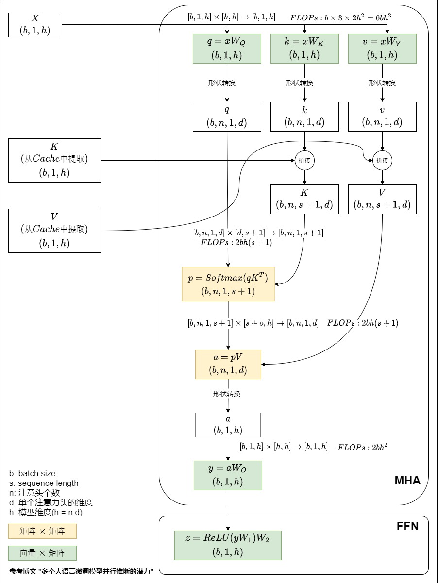
Source-local figure: author-created for A16 from the cached MHA decode derivation. M4.1 retains it as a historical trace; the running GQA fixture and M5 cache-runtime contracts are stated separately.

Source-local figure: A16 - Resource Consumption. It uses an MHA-style H_{kv}=H_q cache and a historical two-matrix ReLU FFN. M4.1’s running fixture instead uses GQA and SwiGLU, so the figure supplies execution order, not the fixture’s exact widths or coefficients.

Decode is arithmetically smaller than full prefill for one request, but it has a different pressure:

every new token reads the cached K/V history
the cache grows with T
many requests need separate or shared cache allocation
batching is constrained by cache memory

This is why M4 cannot stop at “attention is quadratic.” In prefill/training, the large square score/probability domain is the obvious materialization cliff. In decode, S_q=1, but the growing K/V object becomes persistent input state.

0x09C Stored KV Bytes Are Not Automatically DRAM Reads

The KV cache stores previous keys and values so decode does not recompute the full prefix for every generated token.

Logical per-layer cache shapes:

K_cache: [B, T, H_kv, d_h]
V_cache: [B, T, H_kv, d_h]

The all-layer byte formula is:

$$M_{KV}=BTL(2H_{kv}d_h)b$$

Variable units:

B      active sequences
T      cached tokens per sequence
L      layers
2      K and V
H_kv   key/value heads
d_h    scalars per head
b      bytes per scalar

For the running configuration at T = S = 4096:

M_KV = B * T * L * 2 * H_kv * d_h * b
     = 1 * 4096 * 32 * 2 * 8 * 128 * 2
     = 536,870,912 bytes
     = 0.50 GiB

Per cached token, per sequence:

2 * H_kv * d_h * b * L
= 2 * 8 * 128 * 2 * 32
= 131,072 bytes
= 128 KiB

At T = 32768:

32768 * 128 KiB = 4.00 GiB

That is the stored cache ledger for one active sequence under H_kv=8, bf16/fp16 cache, and no allocator overhead. Storage alone does not say whether the next kernel obtains bytes from L2, HBM, host memory, or a remote rank.

0x09D Rectangular Attention Derives A K/V Input Ledger

Let one attention call have S_q query rows and S_k visible K/V rows. The two pairwise contractions request:

$$\begin{aligned} F_{QK^T}&=2BH_qS_qS_kd_h,\\ F_{PV}&=2BH_qS_qS_kd_h,\\ F_{\text{pairwise}}&=4BH_qS_qS_kd_h. \end{aligned}$$

If a grouped kernel reads each logical K/V value once across the selected boundary and shares it across all query heads in its group, the K/V input payload is:

$$Q_{\text{KV input,1pass}} =2BH_{kv}S_kd_hb_{kv}.$$

The K/V-input-only arithmetic intensity is therefore:

$$\begin{aligned} I_{\text{KV-only}} &=\frac{4BH_qS_qS_kd_h} {2BH_{kv}S_kd_hb_{kv}}\\ &=\frac{2S_q}{b_{kv}}\frac{H_q}{H_{kv}}. \end{aligned}$$

This ratio omits Q/output movement, score/normalizer state, masks, new-cache writes, paging metadata, and repeated physical K/V loads. It is an ideal reuse diagnostic, not total kernel intensity.

For one-token decode in the running GQA fixture:

B=1, S_q=1, S_k=32768
H_q=32, H_kv=8, d_h=128, b_kv=2

pairwise attention work/layer:
    4 * 1 * 32 * 1 * 32768 * 128
    = 536,870,912 FLOPs

one-pass logical K/V input/layer:
    2 * 1 * 8 * 32768 * 128 * 2
    = 134,217,728 bytes
    = 128 MiB

K/V-only intensity:
    536,870,912 / 134,217,728
    = 4 FLOP/byte

all 32 layers, if every history is consumed once:
    32 * 128 MiB = 4.00 GiB logical K/V input/token

The equality between 4.00 GiB stored and 4.00 GiB one-pass input occurs because this particular decode step consumes the full history once at every layer. It does not prove 4.00 GiB of measured HBM reads. Physical traffic can be higher when query-head workers reload shared K/V or lower at the DRAM boundary when caches satisfy some requests.

S_k cancels from the ratio but not from work or bytes. Doubling context length doubles both numerator and denominator and can still nearly double attention time.

If the model used full MHA with H_kv = H_q = 32, the same ledger becomes:

H_kv = 32 instead of 8
=> 4x larger
=> 16.00 GiB at T = 32768

The GQA paper frames grouped-query attention as an intermediate architecture between MHA and MQA and studies an uptraining path from MHA checkpoints. In the running byte contract, changing H_{kv} gives:

Architecture	H_q	H_{kv}	Cache at T=32768,L=32	Ideal one-row K/V-only intensity
MHA	32	32	16.00 GiB	1 FLOP/byte
running GQA	32	8	4.00 GiB	4 FLOP/byte
MQA	32	1	0.50 GiB	32 FLOP/byte

The storage reduction is architectural. The traffic/intensity improvement is conditional on a kernel that shares one K/V load across the corresponding query group instead of physically repeating K/V to H_q workers. Quality, checkpoint conversion, training, tensor-parallel replication, and cross-layer sharing are owned by M5.7.

0x09E Design Alternatives Change Different Rows

Choice	State consequence	Work/transfer consequence	Owner after this ledger
recompute the growing prefix without KV cache	no persistent projected history	old-token projections and attention are executed again	historical baseline only
cache exact K/V	O(TLH_{kv}d_h) persistent values	read visible history and append one row	M5.1 lifecycle
MHA / GQA / MQA	changes H_{kv} and checkpoint architecture	changes K/V payload; physical reuse remains a kernel claim	M5.7
final-row versus all-row logits	no change to attention cache	changes R_{logits}dV vocabulary work and logits payload	M3.8 interface
paged, static, offloaded, or shared cache	can change reservation and placement, not logical K/V elements	adds address translation, movement, or reuse behavior	M5.2-M5.6
multi-token verification or chunked decode	S_q>1 temporary rows	raises pairwise work and potential reuse per K/V byte	M7

The no-cache baseline and cache-enabled decode are mathematically equivalent only when both reconstruct the same K/V values, masks, positions, and logits. They are not equivalent cost schedules.

0x09F Executable Phase And Rectangular-Attention Trace

def phase_record(mode, S, T_past=0, requested_logits="final"):
    if mode == "training":
        return Phase(S_new=S, S_q=S, S_k=S,
                     read_cache=False, write_cache=False,
                     retain_backward=True, logits="all_supervised")
    if mode == "prefill":
        return Phase(S_new=S, S_q=S, S_k=S,
                     read_cache=False, write_cache=True,
                     retain_backward=False, logits=requested_logits)
    if mode == "decode":
        return Phase(S_new=1, S_q=1, S_k=T_past + 1,
                     read_cache=True, write_cache=True,
                     retain_backward=False, logits="final")
    raise ValueError(mode)


def rectangular_attention_ledger(B, Hq, Hkv, Sq, Sk, dh, bkv):
    pairwise_flops = 4 * B * Hq * Sq * Sk * dh
    kv_input = 2 * B * Hkv * Sk * dh * bkv
    return {
        "pairwise_flops": pairwise_flops,
        "kv_input_1pass": kv_input,
        "kv_only_intensity": pairwise_flops / kv_input,
    }

Mechanical closure:

d = rectangular_attention_ledger(
    B=1, Hq=32, Hkv=8, Sq=1, Sk=32768, dh=128, bkv=2
)
assert d["pairwise_flops"] == 536_870_912
assert d["kv_input_1pass"] == 134_217_728
assert d["kv_only_intensity"] == 4
assert 32 * d["kv_input_1pass"] == 4_294_967_296

The code still does not know HBM traffic. It emits a falsifiable logical row for a profiler or runtime trace to reconcile later.

0x09G Failure Lab And Publish Gate

Failure	Hidden contract error	Repair
call stored bytes HBM traffic	residency confused with transfers	emit directional transfer rows and a selected tier
call one-pass payload measured traffic	cache, sectors, fusion, and replay disappear	attach profiler counters as a separate observation
label every M=1 operator bandwidth-bound	machine and implementation omitted	report low analytical intensity; measure the kernel
reuse 2M/b outside the weight-dominated regime	activation terms silently dropped	retain MK+KN+MN or state the asymptotic regime
use MHA K/V bytes for a GQA fixture	H_q substituted for H_{kv}	derive stored K/V axes from the manifest
say context is free because S_k cancels from intensity	ratio mistaken for absolute cost	report both FLOPs and K/V bytes, each linear in S_k
treat training and prefill as the same call	backward liveness and cache writes disappear	record phase state and output policy
project all prompt logits for a final-row API	output contract omitted	bind R_{logits} to the interface
derive online softmax here	M4.3 algorithm ownership duplicated	stop at the global S/P transfer rows
turn cache bytes into a serving-capacity claim	allocation and scheduler state omitted	hand the logical object to M5

Publish gate:

every byte claim names storage, liveness, scheduled transfer, or observation
the GEMM intensity formula states its one-pass and tier assumptions
materialized GQA attention and M4.3's MHA fixture are not mixed
training, prefill, and decode have explicit row/state/output contracts
stored KV bytes and one-pass K/V input are separate ledgers
M4.2, M4.3, M4.5, M5, and M7 boundaries remain explicit

M5 will turn this cache object into a serving system:

allocation
paging
prefix reuse
lossy retention
offload
prefill/decode placement
scheduler admission

M4.1 only establishes the bytes and shapes.

0x0A Executable Estimator And Reconciliation

The previous sections established formulas and accounting boundaries. They are still vulnerable to a familiar failure: a copied dimension, an omitted alias, or a changed output policy can leave the prose internally plausible while the numbers no longer describe the declared model.

The owner question is therefore operational:

Can an independent observation falsify a manifest-derived ledger without the estimator rewriting either side to make them agree?

The checked-in estimator answers with three separate artifacts:

analytical manifest
    -> deterministic prediction ledgers

independent observation bundle
    -> named state entries and scoped counters

reconciliation report
    -> exact, explained, unexplained, or unmeasured

The implementation and fixtures live under:

docs/numinens-evidence/m4-1-cost-estimator/

They use only the Python standard library. The tiny fixture is a synthetic contract test, not a PyTorch execution, accelerator profile, or latency benchmark.

0x0AA Prediction And Observation Have Separate Provenance

A prediction is not an observation with missing fields filled in. The estimator keeps the two records separate:

Record	Contains	Authority	Forbidden shortcut
analytical manifest	architecture, phase, dtypes, state policy, liveness events, transfer boundary	declared model and accounting contract	infer missing architecture from a counter
prediction	parameter, state, activation, FLOP, K/V, and transfer ledgers	deterministic functions over the manifest	tune a formula to close a residual
observation	names, shapes, dtypes, aliases, scoped counters, producer metadata	independent fixture, source, or run artifact	rename keys silently until they match
reconciliation	field diffs and signed residuals	comparison only	mutate prediction or observation

Evidence status is part of the schema, not editorial decoration:

synthetic_contract_test
    deterministic schema, equation, alias, transition, and residual test

source_reported
    pinned external result with its source URL and original scope

locally_measured
    named hardware/framework environment plus raw artifacts and scoped counters

unmeasured
    analytical manifest or incomplete observation with no performance claim

A record labeled locally_measured is rejected if hardware, framework, or raw artifact fields are missing. A source_reported record requires its source URL. This prevents an analytical fixture from acquiring empirical authority by passing through a profiler-shaped JSON schema.

0x0AB Parse And Reject Before Counting

The tiny manifest declares the full accounting object rather than passing a loose collection of dimensions:

{
  "architecture": {
    "num_layers": 2,
    "hidden_size": 8,
    "num_attention_heads": 4,
    "num_key_value_heads": 2,
    "head_dim": 2,
    "intermediate_size": 12,
    "vocab_size": 16,
    "tie_word_embeddings": true
  },
  "workload": {
    "phase": "prefill",
    "batch_size": 1,
    "new_tokens": 4,
    "query_tokens": 4,
    "visible_kv_tokens": 4,
    "logit_rows": 1,
    "attention_plan": "materialized"
  },
  "evidence_class": "synthetic_contract_test"
}

Validation runs before tensor construction:

def validate_manifest(m):
    require(m.schema_version == "numinens.m4-1-cost-manifest.v1")
    require(m.H_q * m.d_h == m.d)
    require(m.H_q % m.H_kv == 0)
    require(m.phase in {"training", "prefill", "decode"})
    require(all(dtype.bytes_per_value > 0 for dtype in m.numeric_roles))
    require(unique(role.name for role in m.state_policy))

    if m.phase == "decode":
        require(m.new_tokens == 1 and m.query_tokens == 1)

The tensor-name adapter is deliberately fixture-specific and Llama-like. A different implementation needs an explicit adapter from its configuration and checkpoint schema. It must not be handled by silently rewriting unexpected keys until aggregate counts agree.

0x0AC One Manifest Feeds Every Analytical Ledger

The executable estimator has one pure derivation function per accounting question:

architecture_tensor_rows()          stored names, axes, dtype, aliases
parameter_ledger()                  named, unique, trainable, buffers
training_state_ledger()             state role x basis x dtype x copies
activation_liveness()               event replay and peak live cut
forward_flop_ledger()               contractions under the 2-FLOP FMA rule
kv_cache_ledger()                   logical rectangular K/V payload
materialized_attention_transfer()   selected schedule boundary

For the two-layer tiny fixture, the independently asserted summary is:

Ledger	Derived value	Contract
named parameter occurrences	1,256 scalars	tied names still appear twice
unique/trainable parameters	1,128 scalars	tied storage counted once
parameter payload	2,256 bytes	bf16 unique parameter storage
declared six-class training state	22,560 bytes	exactly 20 bytes per unique trainable scalar
activation live peak	448 bytes	supplied events plus event-local workspace
forward matmul/pairwise work	8,960 FLOPs	two blocks plus one final-row head
logical K/V payload	128 bytes	two layers, four visible tokens
materialized attention transfer	1,408 bytes	eight directional rows per layer

The FLOP path is reconstructible rather than opaque:

per layer:
    Q/K/V/O projections = 1,536 FLOPs
    QK^T and P V         =   512 FLOPs
    SwiGLU projections   = 2,304 FLOPs
    layer subtotal       = 4,352 FLOPs

two layers               = 8,704 FLOPs
one-row vocabulary head  =   256 FLOPs
total                    = 8,960 FLOPs

The transfer trace also exposes an easy shape error. For [B,H_q,S_q,S_k]=[1,4,4,4], a score or probability tensor has 64, not 32, elements. At two bytes per value:

per materialized layer:
    Q read                         64 bytes
    K read                         32 bytes
    S write + read            2 * 128 bytes
    P write + read            2 * 128 bytes
    V read                         32 bytes
    O write                        64 bytes
    total                         704 bytes

two layers                      1,408 bytes

The point of executable closure is not that Python arithmetic is intrinsically trustworthy. It is that every term has a named source axis and an independent expected value that can fail.

0x0AD Liveness Is Replayed, Not Summed

The tiny liveness fixture supplies allocate and release events. It does not ask the estimator to infer a framework graph:

Event	Live tensor payload	Workspace	Total
hidden input	64 B	0 B	64 B
Q, K, V ready	192 B	0 B	192 B
score GEMM	320 B	128 B	448 B
probability ready while score remains live	448 B	0 B	448 B
score released, attention output allocated	384 B	0 B	384 B

This is a logical tensor-plus-declared-workspace peak. It is not allocator reserved memory, process memory, or device-used memory. If the running manifest contains no liveness events, the estimator returns not supplied; zero would incorrectly claim that the physical peak had been measured and found empty.

0x0AE State-Dict Reconciliation Is Schema-First

PyTorch’s state_dict contains parameters and persistent buffers under state keys. It is a shallow mapping to underlying objects, so names and storage identity answer different questions. The synthetic observation records both:

model.embed_tokens.weight  shape=[16,8]  alias=storage:token-embedding
lm_head.weight             shape=[16,8]  alias=storage:token-embedding

The reconciler checks:

missing and unexpected names
duplicate names
shape, dtype, parameter/buffer kind, and trainability
expected tied aliases
accidental alias collisions across expected storages
named-occurrence and unique-storage scalar totals

The exact result is therefore not merely 1,128 == 1,128:

observed named occurrences = 1,256 scalars
observed unique storage    = 1,128 scalars
expected tie group         = {embedding, lm_head}
schema and alias status    = exact

A shape mutation from [8,8] to [4,16] preserves 64 scalars and still fails reconciliation. Aggregate parameter count cannot prove that the stored axes or contraction are correct.

The combine step is a diff, not a repair:

def reconcile_state(expected_rows, observed_rows):
    compare_names_shapes_dtypes_kinds_and_trainability()
    compare_expected_and_observed_alias_groups()
    report_named_occurrences_and_unique_storage_separately()
    return exact_or_open_diff

The report does not mutate P or O; it only records whether their declared objects reconcile.

0x0AF Residuals Are Outputs, Not Correction Terms

For a counter j, define:

$$r_j = O_j - P_j, \qquad e_j = \sum_i E_{j,i}$$

where P_j is the analytical prediction, O_j the independent observation, and E_{j,i} signed explanation rows. A comparison closes only when:

$$r_j = 0 \qquad\text{or}\qquad e_j = r_j$$

The synthetic observation deliberately exceeds both predictions:

Counter	Prediction	Observation	Residual	Explanation	Status
allocator-like peak	448 B	576 B	+128 B	padding and unmodeled temporary +128 B	explained
selected transfer boundary	1,408 B	1,536 B	+128 B	synthetic sector padding +128 B	explained

If the explanation is changed to 64 B, the residual remains 128 B and the report stays open. The prediction remains 448 B or 1,408 B; reconciliation does not add the unexplained bytes back into the formula.

def reconcile_counter(prediction, observation, explanations):
    residual = observation - prediction
    explained = sum(row.bytes for row in explanations)
    status = (
        "exact" if residual == 0
        else "explained" if explained == residual
        else "unexplained"
    )
    return prediction, observation, residual, explained, status

0x0AG Observation Visibility Is Part Of The Counter

Framework tools observe different boundaries:

Observation path	Useful evidence	Visibility limit that must remain attached
state_dict or named traversal	keys, shapes, dtypes, persistent buffers, alias relations	not activation liveness, allocator reserve, or kernel traffic
PyTorch CUDA memory snapshot	allocator segments, blocks, allocation history, stack context	memory outside the PyTorch allocator can be invisible; NCCL is a documented example
torch.profiler	operator timing, shapes, memory activity, stacks, selected formula-estimate FLOPs	not a universal hardware-operation or HBM-transaction oracle
device/process counter	broader device-used or process scope	does not identify which tensor or operator caused the bytes

The observation schema therefore requires a human-readable visibility field for every counter. A locally measured extension should additionally pin the framework and driver versions, accelerator model, backend, input shape, attention implementation, warmup and capture policy, and raw artifact path.

The checked-in bundle says explicitly:

synthetic allocator-like tensor payload;
no driver, external allocator, or hardware observation

synthetic profiler-like selected-boundary counter;
not a DRAM measurement

These are contract fixtures whose purpose is to test reconciliation behavior. They are not evidence about a GPU.

0x0AH Rejection Tests Are Part Of The Estimator

The test suite includes closure and adversarial cases:

Mutation	Why aggregate arithmetic can miss it	Required result
Q weight [8,8] -> [4,16]	both contain 64 scalars	open: stored-axis mismatch
give lm_head a separate alias	named shapes still match	open: expected tying broken
explain only 64 B of a 128 B residual	a narrative explanation exists	open: residual not closed
label evidence locally measured without hardware/raw artifacts	counter shape looks plausible	reject the observation schema
omit the observation bundle	analytical ledgers still derive	report unmeasured, not measured or exact

Run the complete fixture:

python3 docs/numinens-evidence/m4-1-cost-estimator/test_cost_estimator.py

The eight tests exercise exact closure, tied storage, same-numel shape failure, broken aliases, unexplained residuals, invalid evidence labels, the unmeasured path, and the running-configuration smoke contract.

0x0AI The Running Fixture Is An Unmeasured Smoke Report

The same parser can ingest the article’s running configuration:

L=32, d=4096, H_q=32, H_kv=8, d_h=128,
d_ff=14336, V=128256, untied embedding/head,
B=1, S_new=S_q=S_k=4096, final-row logits, bf16

Its executable summary reconciles the earlier sections:

Ledger	Exact analytical output	Scope
one decoder block	218,112,000 parameters	GQA + SwiGLU + two RMSNorm scales
32-block stack	6,979,584,000 parameters	embeddings/head excluded
complete declared model	8,030,261,248 parameters	untied embedding and head included
bf16 parameter payload	16,060,522,496 B	parameter-only lifecycle policy
forward matmul/pairwise work	65,971,748,339,712 FLOPs	32 prefill blocks + final-row head
logical K/V payload	536,870,912 B = 0.5 GiB	four thousand ninety-six visible tokens
materialized attention schedule	140,123,308,032 B = 130.5 GiB	all 32 layers at the declared boundary
activation peak	not supplied	no event trace in this smoke manifest
observation status	unmeasured	no checkpoint, allocator, profiler, or run bundle

The forward subtotal per layer remains the derivation from 0x05:

Q/K/V/O projections:       343,597,383,680 FLOPs
QK^T and P V:              274,877,906,944 FLOPs
SwiGLU projections:      1,443,109,011,456 FLOPs
per-layer subtotal:      2,061,584,302,080 FLOPs

This report does not claim a model file size, training peak, achieved FLOP/s, latency, or measured HBM traffic. The exact output is useful precisely because undeclared quantities remain absent rather than being replaced by zeros.

0x0AJ Executable Contract And Publish Gate

The estimator command fails on a fixture mismatch or open reconciliation:

python3 docs/numinens-evidence/m4-1-cost-estimator/cost_estimator.py \
  docs/numinens-evidence/m4-1-cost-estimator/manifest_tiny_tied.json \
  --observation docs/numinens-evidence/m4-1-cost-estimator/observation_tiny_tied.json \
  --fail-on-mismatch

Its current ownership boundary is deliberate:

included:
    Llama-like GQA/SwiGLU tensor schema
    tied-storage reconciliation
    declared training-state classes
    supplied activation-liveness events
    dense matmul and pairwise-attention FLOPs
    logical K/V payload
    materialized-attention schedule rows

not inferred:
    framework graph and saved tensors
    allocator reserve or external allocations
    actual cache-line or HBM transactions
    runtime latency and throughput
    parallel ownership transformations

Publish gate:

the manifest is validated before counting
all ledgers derive from the same immutable manifest
state reconciliation checks axes, dtype, kind, trainability, and aliases
prediction and observation retain independent provenance
every counter names its visibility boundary
residual explanations close arithmetically or remain open
missing liveness and observations remain not supplied or unmeasured
synthetic, source-reported, locally measured, and unmeasured evidence do not mix

0x0B Paper-By-Accounting-Contract Comparison

The owner question is not “which paper has the right FLOP number?” It is:

What object did each source count, under which architecture, phase, backward, replay, state, and ownership contract?

The distinction matters because the same symbols are overloaded. Kaplan’s B is a token batch and its S is an update count. This article usually uses B for sequence batch and S for sequence length. PaLM’s “model FLOPs” and “hardware FLOPs” deliberately use different replay boundaries. Korthikanti et al. primarily model saved activation bytes, not another interchangeable 6ND training total.

0x0BA Normalize Coordinates Before Numbers

A source-reported value is not ready for cross-paper comparison until this record is complete:

architecture:
    attention type, FFN type/width, layers, hidden size, vocabulary

parameter coordinate:
    unique checkpoint state, non-embedding N, total N, or executed matrices

phase and rows:
    training/prefill/decode, token presentations, all-row/final-row logits

operation set:
    projections, pairwise attention, softmax, head, non-matmul primitives

backward:
    need_dX, need_dW, and the multiplier actually derived from them

recomputation:
    named replay region and replay count

state and liveness:
    persistent classes or saved tensors at a named lifecycle point

parallel ownership:
    global versus rank-local object, process group, and schedule

output and evidence:
    scalar/FLOP/byte unit, analytical/source-reported/measured status

Let normalize(source_claim, target_manifest) produce either a complete mapping or an open difference set. Numeric comparison is allowed only in the first case:

def comparison_gate(source_claim, target_manifest):
    mapping = normalize_every_contract_axis(source_claim, target_manifest)
    if mapping.open_differences:
        return {"status": "not_comparable", "open": mapping.open_differences}
    return {"status": "normalized", "target_case_id": target_manifest["case_id"]}

This is stricter than attaching a paper title to a number. It makes the coordinate transformation inspectable.

0x0BB A16 Is A Composite Source, Not One Contract

A16 combines several useful but different accounting objects:

parameter and mixed-precision state examples
Korthikanti-style saved-activation coefficients
Kaplan-style non-embedding compute
Megatron-style checkpoint-aware iteration FLOPs
inference arithmetic-intensity and K/V discussions

That breadth is useful pedagogically, but it means “the A16 formula” is not a single coordinate. Each subsection must be bound to its inherited source and assumptions. M4.1 preserves A16 as source-local provenance while correcting the extra +2BShV appended after Megatron Equation 3: the primary equation’s V/(16Lh) term already expands to the head’s forward-plus-backward 6BShV.

0x0BC The Six Contracts

The complete checked-in registry is docs/numinens-evidence/m4-1-cost-estimator/paper_contracts.json. The table below is its human-readable projection.

Source	Primary accounting object	Parameter and operation coordinate	Backward and replay	State / ownership boundary
A16	composite teaching article: scalars, bytes, FLOPs, and transfer examples	coordinate changes by subsection; inherited dense-MHA/4h examples cannot be silently applied to GQA/SwiGLU	several backward and recomputation policies appear; normalize each subsection independently	mixes global and parallel examples; source-local, not one closed paper contract
Kaplan et al.	non-embedding model-size coordinate and training-compute proxy	N excludes vocabulary/position embeddings; Table 1 shows context attention, while headline 6N drops it for the studied regime	backward approximately 2x forward; no separate replay term	global non-embedding FLOPs, not memory or rank-local state
Hoffmann et al.	detailed training FLOPs compared with 6ND	includes embedding matrices; Appendix F adds projections, pairwise attention, softmax, dense block, and final logits	detailed forward multiplied by three; no separate rematerialization row	global arithmetic; Table A4’s ratio is architecture-dependent
PaLM	model-FLOP and hardware-FLOP utilization denominators	6N parameterized matmuls plus 12LHQT dense attention per token	model FLOPs exclude replay; hardware FLOPs add declared selective rematerialization	combines global arithmetic with observed throughput and aggregate peak only after denominator selection
Megatron	lower-bound GPT GEMM FLOPs per training iteration	classic MHA, two-matrix 4h FFN, pairwise attention, and all-row vocabulary head	blocks use forward + two backward + one replay; head uses forward + two backward, no replay	global model FLOPs; communication and runtime inefficiency are outside Equation 3
Korthikanti et al.	saved-activation bytes plus model-versus-hardware FLOPs	classic MHA/GeLU saved-tensor ledger with two-byte values and one-byte dropout masks in leading coefficients	model FLOPs use forward + two backward; selective hardware FLOPs replay attention work	TP/SP/PP and first-stage pipeline pressure are explicit; allocator/workspace is absent

Korthikanti’s contract demonstrates why a one-row “paper FLOPs” table would be wrong. Its baseline saved-activation result is

$$M_{act,layer}=sbh\left(34+\frac{5as}{h}\right)\ \text{bytes},$$

under the paper’s tensor and representation assumptions. With tensor plus sequence parallelism and the paper’s first-stage pipeline schedule, the leading total becomes

$$M_{act,stage0}=\frac{sbhL}{t} \left(34+\frac{5as}{h}\right).$$

Selective recomputation removes the saved quadratic-attention term from that leading memory ledger, while Appendix A adds the replayed attention work to a separate hardware FLOPs expression. This is a memory-policy comparison and a replay accounting contract, not a substitute for Kaplan’s scaling-law coordinate.

0x0BD Similar Formulas, Different Design Choices

The sources expose alternatives rather than a linear progression toward one formula:

Decision	Alternative A	Alternative B	What must remain separate
compute coordinate	6ND proxy	architecture-shaped operation sum	convenience versus operation completeness
replay denominator	model FLOPs	hardware FLOPs including replay	model work versus executed work
activation policy	retain backward dependencies	replay named regions	saved bytes versus extra arithmetic/traffic
parameter set	non-embedding N	total/unique/executed matrices	empirical coordinate versus storage/operation coordinate
output-head policy	all training rows	final inference row	same stored matrix, different row count
parallel view	global logical work	rank-local resident/transient state	conservation versus placement and schedule

The registry deliberately sets cross_paper_numeric_comparison_allowed=false for all six entries. A title, formula resemblance, or close numerical ratio cannot open that gate.

0x0BE Paper-Contract Publish Gate

all six required contracts are present and source-scoped
A16 is identified as a composite local source
paper symbols are translated before reuse
operation, backward, and replay sets are explicit
activation bytes are not compared as if they were training FLOPs
model FLOPs and hardware FLOPs retain separate denominators
global arithmetic is not relabeled as rank-local runtime
numeric comparison remains closed without a target manifest

0x0C Worked Ledger And Sensitivity Surface

Sensitivity analysis asks a different question from reconciliation. The executable reconciliation chapter asked whether one prediction and one independent observation agree. This section asks how the analytical prediction changes when one declared control field changes and all other manifest state remains fixed.

0x0CA Base Running Contract

The immutable base is running-gqa-swiglu-prefill-unmeasured:

architecture:
    L=32, d=4096, Hq=32, Hkv=8, dh=128
    dff=14336, V=128256, untied token/output weights

workload:
    prefill, B=1, Snew=Sq=Sk=4096
    final-row logits, materialized attention schedule

representations:
    bf16 parameters, activations, K/V, scores, probabilities

ownership:
    world=1, replicated parameter payload

evidence:
    analytical and unmeasured

Its executable base report is:

Ledger	Exact value	Human-scale reading
unique learned scalars	8,030,261,248	8.030B
parameter payload	16,060,522,496 B	14.96 GiB
ideal rank-local parameter payload	16,060,522,496 B	14.96 GiB
forward dense/pairwise matmuls	65,971,748,339,712 FLOPs	65.972 TFLOPs
rectangular logical K/V payload	536,870,912 B	0.50 GiB
materialized-attention scheduled transfer	140,123,308,032 B	130.50 GiB
activation peak	not supplied	no liveness claim

No row is measured. The table is the common origin from which the deltas below are derived.

0x0CB One Declared Field, One New Prediction

For base manifest $m$, output ledger $y$, and one declared field $x_i$, each case computes

$$\Delta_i y = y\!\left(m[x_i\leftarrow x_i']\right)-y(m),$$ $$R_i y = \frac{y\!\left(m[x_i\leftarrow x_i']\right)}{y(m)}.$$

The runner deep-copies the base, applies exactly one patch, validates the new manifest, derives every ledger again, and verifies the base SHA-256 afterward. A representation or parallel policy is one declared object-valued field, so its internal dtype/bytes or world/shard leaves move together rather than forming an invalid half-policy.

base_hash = canonical_digest(base_manifest)
scenario = deepcopy(base_manifest)
apply_exactly_one_declared_patch(scenario, case.patch)
prediction = estimate(scenario)
assert canonical_digest(base_manifest) == base_hash

The suite rejects a second patch. It also rejects unsupported paths, no-op patches, invalid head divisibility, and shard degrees that do not divide the world size.

0x0CC Sensitivity Results

Ratios below are relative to the base. A dash means that the ledger is invariant, not that the runtime effect is zero.

Single control-field change	Unique parameters	Parameter payload	Forward matmuls	Logical K/V	Materialized transfer
Hkv: 8 -> 32 (MHA)	1.100x	1.100x	1.100x	4.000x	1.011x
Hkv: 8 -> 1 (MQA)	0.971x	0.971x	0.971x	0.125x	0.997x
untied -> tied token/head storage	0.935x	0.935x	1.000x	1.000x	1.000x
parameter representation 2 -> 4 B	1.000x	2.000x	1.000x	1.000x	1.000x
batch 1 -> 8	1.000x	1.000x	8.000x	8.000x	8.000x
visible K/V context 4096 -> 8192	1.000x	1.000x	1.133x	2.000x	1.985x
final-row -> all-row logits	1.000x	1.000x	1.065x	1.000x	1.000x
K/V representation 2 -> 1 B	1.000x	1.000x	1.000x	0.500x	0.998x
replicated -> ideal 8-way parameter shard	1.000x	1.000x	1.000x	1.000x	1.000x

The final row changes the separate ideal rank-local parameter payload from 14.96 GiB to 1.87 GiB (0.125x). Global parameter payload remains 14.96 GiB. The row does not divide workspaces, activations, optimizer state, padding, or transient all-gathers by eight.

0x0CD Why The Ratios Take These Values

Changing Hkv changes the K and V projection widths $d_{kv}=H_{kv}d_h$. Q and O retain $H_qd_h=d$. Therefore the unique parameter delta is

$$\Delta P_{KV}=L\left(2d d_h\Delta H_{kv}\right).$$

For 8 -> 32 heads:

Delta P_KV = 32 * 2 * 4096 * 128 * 24
           = 805,306,368 scalars

Delta bytes at 2 B/scalar
           = 1,610,612,736 B

The K/V payload is directly proportional to Hkv, so it becomes exactly 4x. The materialized schedule barely changes because its dominant rows are the four score/probability writes and reads shaped by Hq, not Hkv.

Tying storage removes exactly one V x d unique matrix:

V*d = 128256 * 4096 = 525,336,576 scalars
saved payload          = 1,050,673,152 B

The head still executes, so forward FLOPs do not change. Likewise, changing the stored parameter representation from two to four bytes doubles payload without changing scalar count or the operation graph.

The batch case scales every declared row count by eight, hence exact 8x ratios for FLOPs, K/V, and this schedule. The context case is different: Snew and Sq stay 4096, while Sk becomes 8192. Projection work stays fixed; pairwise work and score/probability rows double. The resulting whole model forward grows only 1.133x because SwiGLU and projection work still dominate the sum.

All-row logits add

$$2B(4096-1)dV=4{,}302{,}506{,}557{,}440\ \text{FLOPs},$$

which moves the full forward ledger from 65.972 to 70.274 TFLOPs without changing model storage. Halving only K/V value width removes 0.25 GiB from the rectangular K/V object, but just 0.25 GiB from a 130.50 GiB materialized schedule dominated by score/probability traffic. This is why a large improvement in one object can look small in a broader ledger.

0x0CE Alternatives Are Policy Vectors

Real design comparisons often require several coordinated fields. They must not be mislabeled as one-variable sensitivity:

Design comparison	Fields that normally move together	Correct evaluation
MHA -> GQA conversion	K/V head count, checkpoint tensors, quality recovery, kernel grouping	architecture migration plus quality/runtime evaluation
materialized -> online attention	schedule, saved state, replay policy, kernel/backend	compare operation-equivalent algorithms in M4.3/M4.4
BF16 -> quantized weights	payload, scale/zero-point metadata, packing, dequantization, kernels	M8 representation and deployment contract
DP -> FSDP/ZeRO	process mesh, state-class ownership, materialization, collectives, prefetch	per-rank liveness and communication schedule
final-row -> all-row logits	phase, consumer, row count, loss/sampling contract	compare only within the intended phase

The sensitivity table isolates mechanisms. It does not claim that changing one field is a deployable model transformation.

0x0CF Cross-Ledger Phase Summary

The same architecture stresses different ledgers in different phases. The summary below closes the contracts from 0x03-0x09; it does not replace the phase record or its formulas.

Phase	Row/state contract	Analytical transfer warning	Downstream owner
model load	weights and representation metadata become resident	artifact bytes, device residency, and load traffic are different quantities	M8.9-M8.10
training	S_q=S_k=S; backward state is retained or recomputed	forward payload alone omits saved tensors, replay, gradients, collectives, and optimizer work	M4.1 0x04-0x08
fresh prefill	S new rows; prompt K/V is written; logits policy is explicit	materialized [B,H_q,S,S] rows can dominate the visible schedule	M4.3
one-token decode	S_q=1, S_k=T_past+1; one new K/V row is appended	stored K/V and one-pass K/V input can match numerically without equaling DRAM traffic	M4.5 and M5.1
long-context serving	many ragged request histories coexist	allocation, pages, prefix sharing, eviction, placement, and admission are absent here	M5.2-M5.6
MHA/GQA/MQA serving	H_kv changes the persistent K/V object	lower logical payload improves traffic only when the kernel realizes head-group reuse	M5.7
quantized serving	weights, metadata, accumulators, and K/V may use different formats	smaller stored weights do not prove smaller runtime transactions or end-to-end memory	M8

This table is why “the model is 8B” is not enough.

An 8B model can be:

• too large because weights do not fit;
• too slow because memory traffic dominates;
• too expensive to train because activations and optimizer states dominate;
• too constrained in serving because KV cache limits batch size;
• unexpectedly slow after quantization because kernels unpack or move data poorly.

M4 is where the Transformer becomes a program with resource constraints.

0x0D Failure Modes In Cost Reasoning

The owner question is:

If a contract is wrong, what observable symptom exposes it, which check detects it, and what evidence is required to close the failure?

An untestable warning is not closure. Each failure needs four rows:

injected or observed fault
observable symptom
mechanical or measurement check
closed, explained, open, or unmeasured status

Status vocabulary:

rejected     input contract is invalid; counting never starts
open         a schema difference or residual remains unexplained
unmeasured   no independent observation supports a comparison
explained    a nonzero residual closes through scoped signed rows
exact        compared values or schemas agree without a residual

0x0DA Executable Failure Closure

Failure domain	Fault	Observable symptom	Check and closure rule
tensor schema	reshape Q weight from [8,8] to [4,16] with the same scalar count	total parameters look unchanged while stored axes disagree	state reconciliation compares axes, not only numel; remains open
storage identity	untie lm_head.weight while names and shapes still match	named count matches but unique storage grows	alias-group reconciliation detects the changed storage identity
evidence provenance	label a synthetic bundle locally_measured	no hardware/framework/raw artifact supports the label	observation parser rejects before comparison
counter boundary	compare allocator-like bytes with a tensor-payload prediction	nonzero residual appears	visibility is mandatory; signed explanation rows must sum exactly to the residual
missing evidence	omit the observation bundle	tempting false zero or false pass	status remains unmeasured, never exact
liveness	omit all liveness events	no activation peak can be derived	peak is not supplied, not zero bytes
sensitivity isolation	alter head count and batch in one case	causal attribution is ambiguous	sensitivity parser requires exactly one declared patch
sensitivity immutability	mutate the shared base between cases	later rows depend on case order	deep-copy each case and verify the base canonical SHA-256 afterward
parallel ownership	set shard degree 3 in world size 8	ideal shard is not a legal process-group partition	manifest validation rejects a non-dividing degree
paper comparison	enable numeric comparison on an unnormalized Kaplan row	similar symbols appear comparable without a target coordinate	registry rejects comparison without normalized_to_common_manifest and target_case_id
fixture drift	change a formula or running geometry	expected integer ledger no longer closes	expected_contract mismatch fails --fail-on-mismatch
source coverage	remove one of the six paper contracts	comparison silently loses an incompatible coordinate	registry requires the exact A16/Kaplan/Chinchilla/PaLM/Megatron/Korthikanti ID set

The checked-in suite now contains 14 tests. It includes positive closure fixtures as well as adversarial cases; a suite containing only known-good inputs would verify arithmetic but not fail-closed behavior.

The evidence record is versioned by more than a final number:

manifest schema and case_id
canonical manifest SHA-256
estimator/report schema
paper-contract registry and source locators
sensitivity suite and exactly one declared patch per case
observation producer, visibility, and raw artifact when measured
expected integer fixtures
test command and tool revision

This allows a future formula, framework, or model revision to produce a new record instead of silently changing the meaning of an old result.

0x0DB Reasoning Failures Beyond The Fixture

A cost model becomes useful when it prevents specific mistakes.

Mistake 1:

The weights fit, so inference fits.

Missing ledgers:

KV cache
temporary buffers
allocator reserve
framework workspaces
prefill activation buffers
communication

Mistake 2:

The FLOP count is lower, so it must be faster.

Missing ledgers:

scheduled logical transfer
observed memory transactions
kernel fusion
instruction mix
occupancy
launch overhead
communication

Mistake 3:

Int4 weights mean 4x end-to-end memory reduction.

Missing ledgers:

scales and metadata
KV cache dtype
dequantization path
non-quantized layers
runtime buffers

Mistake 4:

FlashAttention makes attention linear.

Correct ledger:

FlashAttention changes auxiliary memory and the scheduled logical transfer.
Dense attention still computes query-key interactions.

Mistake 5:

GQA is only a model-quality detail.

Correct ledger:

GQA changes H_kv.
H_kv appears in K/V parameters, KV cache bytes, and the ideal decode K/V payload.
Realized DRAM traffic remains a kernel and machine observation.

Mistake 6:

A cache formula is a full serving model.

Missing ledgers:

fragmentation
paging metadata
prefix sharing
eviction/reuse policy
scheduler admission
prefill/decode interference
network transfer under disaggregation

0x0DC Practical Debugging Order

The practical debugging order:

1. Write the tensor shapes.
2. Count elements.
3. Convert to bytes for the chosen dtype.
4. Count matmul FLOPs separately from non-matmul work.
5. Emit scheduled transfer rows for a named memory boundary.
6. Ask whether the phase is training, prefill, or one-token decode.
7. Reconcile those rows with implementation layout, dtype, and observed counters.

That order is slower than a slogan, but it is much harder to fool.

0x0DD Full Article Publish Gate

architecture and workload fields form one immutable manifest
stored tensor axes close against unique and named state counts
dtype and lifecycle point accompany every persistent-state byte row
activation peak comes from liveness, not an indiscriminate sum
forward, backward, and replay regions have separate operation ledgers
global work and rank-local persistent/transient ownership remain distinct
logical transfer, observed transactions, and runtime stay separate
training, prefill, decode, and K/V row extents are explicit
paper values are not compared before all normalization axes close
every sensitivity case changes one declared control field
alternative methods are identified as multi-field policy vectors
every failure has a symptom, check, and evidence status
source-local, externally verified, synthetic, measured, and unmeasured claims do not mix
the executable fixture, source registry, and article numbers agree exactly
every displayed equation has balanced delimiters, named units, and a declared scope
every local post link and image path resolves in the source tree
every responsive picture has a desktop asset, mobile asset, and non-empty alt text
reused source figures identify provenance, figure scope, and rights status
M4.2, M4.3, M4.7, M5, and M8 ownership boundaries remain explicit

0x0E Handoff To GPU Execution And IO-Aware Attention

The cost model has exposed two pressure points:

prefill/training attention:
    S and P can be [B, H_q, S, S]
    materializing them creates activation and scheduled-transfer pressure

decode:
    each step has Q length 1
    but reads a growing K/V cache

M4.2 first establishes the execution vocabulary needed to interpret that pressure:

tensor operation -> kernel launch -> grid/block/warp work
logical bytes -> memory transactions and cache behavior
tile size -> reuse, shared-memory use, registers, and occupancy
runtime claim -> profiler counters and timing evidence

Then M4.3 handles the first attention-specific pressure point.

The question becomes:

Can exact dense attention avoid writing S and P to HBM?

FlashAttention’s core answer:

tile the computation
stream K/V blocks
carry row-local online-softmax state
write compact state and final output instead of full S/P

M4.4 then asks the next question:

After the memory schedule is better, does the kernel expose enough work to the GPU?

That is where FlashAttention-2 enters. M4.5 takes over when one-token decode removes the useful query-row parallelism and backend/cache layout become the local object.

The ownership chain is therefore:

M4.1: logical tensors, phase rows, scheduled transfer, conditional intensity
M4.2: GPU hierarchy, transactions, machine roofline, and profiler evidence
M4.3: exact online softmax and IO-aware attention schedule
M4.4: work partitioning after the IO schedule improves
M4.5: one-token decode kernels and backend/cache-layout boundaries
M5: request-level K/V lifecycle, allocation, sharing, placement, and scheduling
M5.7: MHA/GQA/MQA architecture, quality, conversion, and runtime integration

0xFE Claim Status And Scope

This article uses three claim types:

Claim family	Status	Scope
12d^2, GQA parameter decomposition, 20 bytes / parameter, 34bsh + 5bas^2, A16’s 24BSd^2+4BS^2d dense-MHA/two-matrix-FFN case, A16’s backward/checkpoint explanation, and its Kaplan table reproduction	source-local, rewritten with explicit assumptions	These come from the Transformer Series resource-consumption source article and are treated as accounting cases, not universal laws. A16’s extra +2BShV training term is explicitly corrected against primary Megatron Equation 3 rather than repeated.
original Transformer tying/FFN/position contracts, GLU width matching, LLaMA architectural changes, PyTorch parameter deduplication, autocast and gradient-reset behavior, lazy Adam state, mixed-precision master weights, Adam/AdamW slots, Adafactor geometry, 8-bit optimizer-state representation, autograd saved tensors, activation checkpointing and RNG handling, allocator snapshot visibility, NVIDIA’s FMA-to-2MNK reporting convention, PyTorch profiler’s formula-estimate scope, Kaplan’s non-embedding compute proxy, Chinchilla’s detailed FLOP ledger, Megatron’s replay-aware Equation 3, PaLM’s model-versus-rematerialization FLOP accounting, ZeRO’s cumulative state partitioning, PyTorch FSDP’s regional materialization, Megatron tensor/sequence/context/pipeline axis contracts, NCCL collective semantics, the Full Stack Transformer-inference contraction map, Roofline arithmetic intensity, GQA as an MQA/MHA compromise, and large KV cache as a serving problem	externally anchored	The references below provide primary papers, official framework documentation, or official source code. Optimizer, distributed-wrapper, collective-algorithm, profiler, autograd, allocator, and framework behavior remains version- and policy-specific.
the 1,256-scalar toy ledger, 8,030,261,248-scalar running fixture, unique-versus-state reconciliation method, 12/16/20-byte policy comparison, exact running-fixture state totals, Adafactor gate-projection example, state-lifecycle audit, activation liveness cut, adversarial non-overlap example, 97/17/1 GiB A16-policy projection, checkpoint-policy optimization sketch, 26BSd^2+4BS^2d running-block derivation, exact 32-block and phase-specific output-head ledgers, scalar-chain-rule reconstruction of dX and dW, exact no/selective/block/full-replay training matmul totals, running-fixture 6ND reconciliation, paper-accounting comparison, eight-rank A16-policy DP/ZeRO state projection, FSDP group-liveness examples, ideal-ring communication ledger, TP contraction traces, PP/SP/CP payload examples, legal-causal-versus-scheduled-work split, typed non-matmul ledger, four-ledger byte boundary, 4.078125 GiB materialized-GQA schedule, exact projection row-amortization cases, phase policy, rectangular K/V-input derivation, MHA/GQA/MQA byte comparison, the standard-library manifest estimator, the 1,128-unique/1,256-named tied-state reconciliation, the 448-byte liveness fixture, the 1,408-byte transfer fixture, signed residual-closure tests, the six-source normalized paper-contract registry, nine-case immutable sensitivity surface, 14-test failure-closure suite, the unmeasured running smoke report, and handoff from A16 to FlashAttention/M5	rewrite interpretation, mechanically derived and synthetic-contract tested	These are auditable synthesis ledgers and checked-in contract tests, not benchmark, training recommendation, released-checkpoint, hardware measurement, or measured distributed-runtime claims.

The numeric examples are ledgers. They are not profiler measurements. Real kernels tile, fuse, quantize, cache, overlap, and sometimes choose different layouts. Whenever this article says “pressure,” read it as a shape-and-byte warning, not as a measured latency claim.

0xFF References

• Local source: Exploring the Transformer Series (16) - Resource Consumption
• Local bridge: M1.1 - Architecture and Execution Orientation
• Local bridge: M3.1 - Scaled Dot-Product Attention And The Score Path
• Local bridge: M3.2 - Multi-Head Attention And Head Layout
• Local bridge: M3.6 - FFN/MLP Channel Mixing And Gated Capacity
• Local bridge: M3.7 - Residual, Normalization, And Block Assembly
• Local bridge: M3.8 - Output Head And Logit Interface
• Local bridge: M3.9 - Training Execution: Teacher Forcing, Masks, Loss, And Parallelism
• Local bridge: M3.10 - Single-Request Inference Execution
• Local bridge: M4.2 - GPU Execution Model For Transformer Kernels
• Local bridge: M4.3 - IO-Aware Attention And FlashAttention-1
• Local bridge: M4.4 - FlashAttention-2 Work Partitioning And The Decode Boundary
• Local bridge: M4.5 - Decode Attention Kernels, Mask Programs, And Backend Boundaries
• Local bridge: M4.7 - Empirical Training Scaling Laws And Compute-Optimal Allocation
• Local bridge: M5.1 - Autoregressive Serving State
• Local bridge: M5.7 - MQA, GQA, And K/V Head Sharing
• Local bridge: M6.3 - LoRA, QLoRA, DoRA, And Adapter Serving
• Local bridge: M8.1 - Quantized Numbers, Scales, Zero-Points, And Error
• Local bridge: X1.1 - Unitization and Geometry Metadata
• PyTorch, torch.nn.Linear
• PyTorch, torch.nn.Embedding
• PyTorch, torch.nn.Module parameter, buffer, and state-dict traversal
• PyTorch, torch.amp automatic mixed precision
• PyTorch, Optimizer.zero_grad
• PyTorch, Optimizer.state_dict
• PyTorch, Adam lazy state initialization and slot construction
• PyTorch, Autograd saved tensors and saved_tensors_hooks
• PyTorch, torch.utils.checkpoint
• PyTorch, Understanding CUDA Memory Usage and snapshot visibility
• PyTorch, torch.profiler and with_flops formula-estimate scope
• NVIDIA, Matrix Multiplication Background User’s Guide
• Hugging Face Transformers v5.13.1, LlamaConfig
• Hugging Face Transformers v5.13.1, LlamaAttention, LlamaMLP, and LlamaForCausalLM
• Vaswani et al., Attention Is All You Need
• Noam Shazeer, GLU Variants Improve Transformer
• Hugo Touvron et al., LLaMA: Open and Efficient Foundation Language Models
• Ofir Press and Lior Wolf, Using the Output Embedding to Improve Language Models
• Jianlin Su et al., RoFormer: Enhanced Transformer with Rotary Position Embedding
• Paulius Micikevicius et al., Mixed Precision Training
• Diederik P. Kingma and Jimmy Ba, Adam: A Method for Stochastic Optimization
• Ilya Loshchilov and Frank Hutter, Decoupled Weight Decay Regularization
• Noam Shazeer and Mitchell Stern, Adafactor: Adaptive Learning Rates with Sublinear Memory Cost
• Tim Dettmers et al., 8-bit Optimizers via Block-wise Quantization
• Samyam Rajbhandari et al., ZeRO: Memory Optimizations Toward Training Trillion Parameter Models
• Yanli Zhao et al., PyTorch FSDP: Experiences on Scaling Fully Sharded Data Parallel
• PyTorch, torch.distributed.fsdp.fully_shard grouping, materialization, and communication contract
• Mohammad Shoeybi et al., Megatron-LM: Training Multi-Billion Parameter Language Models Using Model Parallelism
• NVIDIA Megatron Core, Parallelism Strategies Guide
• NVIDIA Megatron Core, Context Parallelism
• NVIDIA NCCL, Collective Operations
• Tianqi Chen et al., Training Deep Nets with Sublinear Memory Cost
• Vijay Korthikanti et al., Reducing Activation Recomputation in Large Transformer Models
• Jared Kaplan et al., Scaling Laws for Neural Language Models
• Jordan Hoffmann et al., Training Compute-Optimal Large Language Models
• Narayanan et al., Efficient Large-Scale Language Model Training on GPU Clusters Using Megatron-LM
• Aakanksha Chowdhery et al., PaLM: Scaling Language Modeling with Pathways
• Sehoon Kim et al., Full Stack Optimization of Transformer Inference: a Survey
• Samuel Williams et al., Roofline: An Insightful Visual Performance Model for Multicore Architectures
• Tri Dao et al., FlashAttention: Fast and Memory-Efficient Exact Attention with IO-Awareness
• Markus N. Rabe and Charles Staats, Self-attention Does Not Need O(n^2) Memory
• Joshua Ainslie et al., GQA: Training Generalized Multi-Query Transformer Models from Multi-Head Checkpoints
• Woosuk Kwon et al., Efficient Memory Management for Large Language Model Serving with PagedAttention