M3.1 — Scaled Dot-Product Attention and Masks: The Score Path Inside One Attention Call
M3.1 — Scaled Dot-Product Attention and Masks: The Score Path Inside One Attention Call
0x00 From Recurrent Alignment To A Batched Score Path
M1.1 traced the long pressure that made attention useful: recurrent encoder-decoder systems had to expose a source sequence to a decoder without forcing every target decision through one fixed summary. M3.1 begins later and asks a narrower implementation question. Once a caller has produced query, key, and value tensors, what exact operation turns them into contextualized value rows?
The active input route is not M2.1 through M3.5. It is:
M2.1 versioned sequence package
    input_ids, valid lengths, segment boundaries, logical positions

M2.2 initial model state
    X0: [B, S, d_model]

M3.1 local attention primitive
    projected Q/K/V + visibility/bias objects -> contextual value rows
M3.1 deliberately studies the local primitive before its caller. It accepts already projected and head-shaped Q/K/V tensors. M3.2 later opens the caller and derives the projections, head split, cross-attention stream ownership, merge, and output projection. This is a bottom-up reading order, not a claim that Q/K/V appear without a producer.
How to read this page. The visible text follows one attention call from start to finish: where the query, key and value tensors come from and what shapes they have, how their scores are formed and scaled, how a mask removes illegal keys before softmax, how softmax turns each row of scores into probabilities, what dropout does to those probabilities, and how they mix the value rows. A three-token example worked by hand (0x09A) and a short reference implementation (0x09B) close that path. Everything else is still here, folded into labelled blocks: derivations, longer worked examples, code, alternative designs and their history, failure cases, framework and runtime details, and the checks behind the article. Each closed block says what it holds and when you would need it. Open a block when you need it; nothing has been removed.
Historical pressure: replace one fixed source summary with an addressable set
The chronology here is selective. It explains the interface inherited by the Transformer; it does not claim that one paper invented every component called attention.
Bahdanau, Cho, and Bengio identified the fixed-length encoder summary as a possible bottleneck and let each decoder step soft-search the encoder annotations. For one available decoder-side query state, the model computed one compatibility score per source annotation, normalized those scores, and formed a weighted context:
The important change was cardinality. The decoder no longer received only one source vector; it received an addressable set and constructed a different soft read for each target step. The paper describes this as an automatic soft search. Whether a learned row corresponds to a human alignment is an empirical claim, not part of the mathematical contract.
Luong, Pham, and Manning made several choices explicit: global attention can score the full source, local attention can restrict the candidate window, and dot, general, or concatenation-based score functions impose different representation and parameter contracts. The query still came from a recurrent decoder state, and source annotations still formed the memory. Attention was a retrieval operation attached to a recurrent sequence model.
The Transformer retained the normalized read but changed its role in the architecture. Learned projections create Q, K, and V roles; many query rows can be evaluated as matrix operations; the dot product is scaled before softmax; and explicit masks define which key rows each query may read. Self-attention uses states from one sequence on both sides of the read, while cross-attention keeps target queries and source key/value rows distinct.
What changed, and what did not
The recurrent and Transformer formulations share a read skeleton but not an execution graph:
| Contract | Recurrent alignment | Transformer attention |
|---|---|---|
| query owner | one available decoder state | one or many projected query rows |
| addressable memory | encoder annotations | projected key rows from the same or another stream |
| score family | often additive, dot, general, or concat | scaled dot product in the canonical primitive |
| legal candidates | global source or a selected local window | explicit boolean/additive visibility over every query-key pair |
| normalization | one distribution over source positions | one distribution over the key axis for every batch/head/query row |
| payload read | weighted source context | weighted projected value rows |
| execution schedule | normally one recurrent target step at a time | all legal query rows can be evaluated together during training/prefill |
The final row-wise contract is therefore still recognizable:
compatibility:
    how strongly this query matches each key

visibility:
    which query-key edges exist for this call

normalization:
    one probability row over legal keys

value mixing:
    use that row to retrieve paired value payloads
What the Transformer adds is a particular tensorization and score convention,
not a different meaning for weighted retrieval. M3.1 derives each part rather
than treating attention as an indivisible metaphor.
Owner question and local object
Owner question: How do projected Q/K/V tensors become masked attention probabilities and contextual value rows?
The complete local object is:
query, key, value
    -> scores = query @ key.T / sqrt(d_k)
    -> optional finite position_bias
    -> visibility mask before softmax
    -> p_attn = softmax(scores, dim=-1)
    -> optional dropout on p_attn
    -> output = p_attn @ value
Further reading Which Transformer Series articles supply this article's code path, mask cases, history and block context; open it to find the original handwritten sources. (about 60 words)
That path is the part A10
implements as attention(query, key, value, mask=None, dropout=None).
A11 supplies the source-local causal,
padding, training/inference, and packing cases that are reconciled at the
score boundary. A1 supplies
the generic read and historical lineage; A2
locates the primitive inside the larger Transformer block.
How this was checked What this article takes from neighbouring articles and leaves to them, and the labels that mark how each claim is supported; open it to see where a related topic is covered. (about 340 words)
Owner contract: consumes, owns, and defers
| Boundary | M3.1 contract |
|---|---|
| consumes from M2.1 | valid lengths, segment/sample boundaries, and logical position metadata from a versioned sequence package |
| consumes from M2.2 | model-width state rows; the M3.2 caller later projects them into Q/K/V |
| accepts from M3.3-M3.5 | optional finite position-bias or transformed Q/K objects without deriving those geometry methods here |
| owns | local score construction, scaling, score-bias addition, visibility application, key-axis softmax, attention dropout, value mixing, local backward flow, and eager/fused semantic parity |
| defers to M3.2 | projection storage, head layout, cross-attention stream ownership, concatenation, and output projection |
| defers to M3.9 | construction of training batches, shifted supervision, and loss masks; M3.1 only consumes the visibility object at the score boundary |
| defers to M4.1/M4.3 | whole-model cost accounting and IO-aware exact-kernel derivation |
| defers to M5.1, M5.2, and M5.3 | persistent request/cache lifecycle in M5.1, multi-request admission and scheduling in M5.2, and physical paging/allocation in M5.3 |
This boundary resolves an apparent mask-ownership conflict. M3.1 does own the attention visibility taxonomy needed to define its score rows, including causal, padding, packed, prefix, window, and cache-shaped examples. It does not own the tokenizer/collator policy that produced lengths and segment IDs, nor the training loop that decides which labels contribute to loss.
Claim status and reading rules
| Label | Meaning in this article |
|---|---|
| Source-local | A1, A2, A10, or A11 directly supplies the explanation, code path, or figure. |
| Externally verified | A primary paper supports the historical or algorithmic claim. |
| Official version-scoped | A framework/API claim is tied to the cited PyTorch or Transformers version. |
| Derivation | The article proves an equation from stated assumptions; it is not attributed to a source merely because the final formula is familiar. |
| Rewrite interpretation | The owner boundary, ledger, or debugging rule is a synthesis used to make implementations auditable. |
| Source-reported | A paper’s observation or benchmark remains attached to that paper and setup. |
| Uncertain | Evidence is insufficient for a general claim; the article must preserve the limitation instead of filling it with intuition. |
The scale, bias, mask, softmax axis, dropout mode, and value multiplication are separate contracts. Same-shape errors survive when those objects are collapsed into one opaque attention label. The remaining sections therefore reconstruct the path one tensor transition at a time.
0x01 The code spine
This is the local object for the whole article:
def attention(query, key, value, mask=None, dropout=None, position_bias=None):
    # query: [B, h, q_len, d_head]
    # key:   [B, h, k_len, d_head]
    # value: [B, h, k_len, d_value]

    d_k = query.size(-1)

    scores = torch.matmul(query, key.transpose(-2, -1)) / math.sqrt(d_k)
    # scores: [B, h, q_len, k_len]

    if position_bias is not None:
        scores = scores + position_bias

    if mask is not None:
        scores = scores.masked_fill(mask == 0, -float("inf"))

    p_attn = scores.softmax(dim=-1)
    # A production eager path may compute this softmax in float32.
    # p_attn: [B, h, q_len, k_len]

    if dropout is not None:
        p_attn = dropout(p_attn)

    out = torch.matmul(p_attn, value)
    # out: [B, h, q_len, d_value]

    return out, p_attn
The original Harvard code uses -1e9 in masked_fill. M3.1 uses -inf to state the semantics: a masked key should be outside the distribution, not merely less preferred.
Everything below is a line-by-line reconstruction of this function.
0x01A Immutable attention-call manifest
A real call fixes more than the code above shows: separate head counts for queries and for keys and values, memory layout, which mask value means “legal”, the precision of each stage, the dropout and random-number state, and which backend actually ran. This section lists those fields and code that rejects an incomplete call; open it when you need to reproduce or compare one specific call. The rest of the page does not depend on it.
Implementation and runtime contracts Every field that identifies one concrete call (head mapping, strides, mask polarity, finite bias, precision per stage, dropout state, requested and observed backend, data lineage), with a schema and validation code. (about 1,670 words, 7 code listings, 2 equations)
The code spine is readable because it suppresses decisions that a real call
cannot suppress. The symbol h does not say whether K/V were stored with the
same number of heads as Q. The name mask does not say whether True means
legal or blocked. float16 inputs do not determine the accumulation dtype of a
fused kernel. An API name such as scaled_dot_product_attention does not by
itself identify the kernel that ran.
Before comparing formulas, implementations, or timings, freeze one call as an immutable manifest. “Immutable” means that these fields describe one concrete execution and cannot change halfway through a derivation or benchmark. It does not mean that every model and backend must choose the same values.
Logical axes and effective head ownership
Use distinct symbols even when a toy self-attention call makes several of them equal:
| Symbol | Meaning |
|---|---|
B | batch rows owned by this call |
Hq | query heads that produce output rows |
Hkv | physically represented key/value heads before any grouping adapter |
Q | query-row count (q_len) |
K | key/value-row count (k_len) |
Dk | query/key feature width used by the score dot product |
Dv | value feature width mixed into each output row |
The immutable tensor ledger is:
| Object and logical shape | Immutable relation |
|---|---|
query[B,Hq,Q,Dk] | owns output rows and the scale width |
key_physical[B,Hkv,K,Dk] | key row j addresses value row j |
value_physical[B,Hkv,K,Dv] | shares B, Hkv, and K with physical keys |
head_map[Hq] integers in [0,Hkv) | maps each query head to one KV head |
key_effectivelogically [B,Hq,K,Dk] | key_physical[:, head_map]; it may remain implicit |
value_effectivelogically [B,Hq,K,Dv] | value_physical[:, head_map]; it may remain implicit |
scoreslogically [B,Hq,Q,K] | one query-by-key row per batch and query head |
visiblebroadcastable to [B,Hq,Q,K] | semantic boolean relation; True means legal |
position_biasbroadcastable to [B,Hq,Q,K] | finite score preference, not legality |
probabilitieslogically [B,Hq,Q,K] | pre-dropout softmax over K |
dropped_probabilitieslogically [B,Hq,Q,K] | training-time stochastic mixing weights |
output[B,Hq,Q,Dv] | one contextual value row per query row |
For ordinary multi-head attention, Hq == Hkv and head_map[h] = h. The code
spine’s shared h axis is exactly this case, or a call after K/V have already
been expanded to the effective query-head axis. With grouped-query or
multi-query attention, M3.2 owns physical projection/storage and the mapping.
The M3.1 equation consumes that mapping. A backend may implement it by a view,
an expand/repeat adapter, indexed grouping, or native grouped-head execution.
Only the logical effective K/V objects are invariant.
This distinction matters for accounting. Repeating K/V into an eager reference tensor is a semantic oracle, not proof that a production kernel stores or moves the repeated tensor.
Storage orientation is not only a shape
The article’s canonical boundary is head-major: [B,H,sequence,feature].
The manifest must additionally record physical shape, stride, device, and
dtype for Q, K, and V. Those fields answer different questions:
logical axis order:
    what each index means

physical strides:
    how the current tensor view walks storage

contiguity:
    whether the next operator can consume that view directly

materialization:
    whether an object receives its own storage at all
key.transpose(-2, -1) denotes a logical [B,H,Dk,K] view for the score
matmul. It is not a claim that checkpoints or KV caches persist a transposed
key. Likewise, scores and probabilities are logical objects even when an
online fused kernel never writes their full [Q,K] matrices to HBM. M4.3 owns
the schedule and IO proof; M3.1 freezes the values that schedule must preserve.
The manifest therefore distinguishes:
qkv_layout = "BHQD"
key_score_view = "transpose last two logical axes"
q_stride, k_stride, v_stride = observed runtime strides
q_contiguous, k_contiguous, v_contiguous = observed booleans
scores_materialized = true | false | backend_internal
probabilities_materialized = true | false | backend_internal
Two calls with equal shapes but different strides can dispatch differently or pay different copies. Two kernels can be semantically equivalent while only one materializes scores. Shape equality is necessary, not a complete execution identity.
Visibility and finite bias are separate objects
M3.1’s canonical semantic object is visible, a boolean relation where
True means the query-key edge exists. It must broadcast to
[B,Hq,Q,K]. A separate query_valid relation, normally broadcastable to
[B,1,Q,1], states whether an output row will be consumed. Key visibility and
query validity are not interchangeable.
position_bias is finite and changes preference among legal keys. Backend
adapters may encode illegality as an additive tensor containing 0 and
-inf, but that tensor is then a visibility encoding, not the finite
position-bias object. The canonical composition is:
Here i indexes a query row and j indexes a key row. In
implementation-oriented form:
scores = (query @ key_effective.transpose(-2, -1)) * (Dk ** -0.5)
biased_scores = scores if position_bias is None else scores + position_bias
masked_scores = biased_scores.masked_fill(~visible, -torch.inf)
probabilities = softmax(masked_scores, dim=-1)
Applying authoritative visibility after the finite preference makes the separation obvious: no later finite positive bias can revive an illegal edge. Loop 4 derives causal, padding, packed, prefix, window, and cache predicates in full. Loop 2 only freezes the interface every one of those designs must reach.
API adapters must name their polarity rather than passing an undocumented
tensor called mask:
| Boundary object | Polarity and adapter into the score path |
|---|---|
M3.1 semantic visible | True means legal; use directly with masked_fill(~visible, -inf) |
| Harvard-style source mask | True means legal; normalize with visible = mask.bool() |
PyTorch functional SDPA boolean attn_mask | True participates; pass semantic visible after broadcast checks |
PyTorch MultiheadAttention binary masks | True is blocked/ignored in the documented mask arguments; invert when converting to semantic visible |
| additive legality bias | 0 is legal and -inf is blocked; add as backend visibility encoding, not finite position bias |
The PyTorch functional SDPA polarity and dropout behavior above are
official version-scoped contracts,
not universal conventions for every attention API. The all-masked-row policy is
also a required manifest field: reject, sanitize_then_zero_invalid_query,
or a named backend behavior that has been tested. Leaving it implicit is not a
valid call specification.
Numerical state is a ledger, not one dtype label
At minimum, record:
| Field | What it controls |
|---|---|
q_dtype, k_dtype, v_dtype | operand storage presented to the local call |
score_accumulation_dtype | dot-product accumulation, if the backend exposes or guarantees it |
bias_dtype | conversion used before adding finite bias or additive visibility |
softmax_accumulation_dtype | exponent/reduction state for normalization |
probability_dtype | dtype presented to value mixing if materialized |
value_accumulation_dtype | accumulation policy for probability-value multiplication |
output_dtype | dtype returned at the M3.1 boundary |
An eager policy may explicitly compute softmax in float32 and cast its result
back to the query dtype. The current version-scoped LLaMA eager path used later
in this article does exactly that. A fused backend may preserve the same output
contract with a different online reduction and without exposing intermediate
dtypes. In that case the manifest records a documented backend guarantee or
backend_internal; it must not guess float32 merely because the eager oracle
uses it.
The same rule applies to arithmetic modes such as TF32, reduced-precision reductions, autocast, and deterministic-algorithm settings. They are execution state, not properties derivable from the attention equation.
Dropout mode includes RNG and returned-weight semantics
dropout_p alone does not identify the operation. Freeze this tuple:
training: true | false
dropout_p: probability in [0,1)
dropout_location: attention probabilities before value mixing
rng_provenance: generator/device plus reproducibility state
returned_weights: none | pre_dropout | post_dropout
For PyTorch’s functional SDPA, a nonzero dropout_p applies dropout even when
the surrounding module is in evaluation mode; the caller must pass 0.0 for
evaluation. Different kernels are not required to consume random numbers in
the same order, so a common seed does not by itself prove bitwise parity.
Semantic parity tests either disable dropout or compare the stated stochastic
contract rather than one sampled mask.
Backend identity has requested and observed parts
backend = "SDPA" is incomplete because the functional entry point can
dispatch among implementations. A reproducible call manifest records:
framework and exact version or source revision
model library and exact version or source revision
entry point
requested backend policy
observed selected backend
device type and architecture
autocast / deterministic / arithmetic-mode state
is_causal flag and external mask kind
dropout mode
return-attention-weights request
compile or graph-capture state
PyTorch documents automatic SDPA backend selection and provides
sdpa_kernel
to constrain eligible implementations. The manifest keeps requested_backend
and selected_backend separate because eligibility is not proof of dispatch.
If selection was not observed, record unobserved; do not relabel it as
FlashAttention from timing intuition. Loop 8 will compare the runtime paths in
detail.
Source-to-tensor lineage
Every local object must have one producer and one consumer contract. The lineage is:
| Producer and object | M3.1 normalization and downstream use |
|---|---|
| M2.1 sequence package valid lengths, segment/sample boundaries, logical positions | compile policy into semantic visible metadata or a backend-equivalent relation; consume at the score-boundary visibility adapter |
M2.2 initial state[B,S,d_model] state rows | no normalization inside M3.1; M3.2 owns the projection caller |
| M3.2 projection/head owner physical Q/K/V plus query-to-KV head mapping | expose canonical axes and the effective head relation; consume in score and value paths |
| M3.3-M3.5 geometry owners, including M3.4 RoPE transformed Q/K and/or finite position bias | verify axis, device, broadcast, and finite-bias contracts; consume before authoritative visibility |
| M3.9 training execution batch visibility policy, training flag, dropout/RNG state | separate attention visibility from label/loss masks; consume in normalization and stochastic value mixing |
| M3.10 single-request execution current query extent, effective key extent, cache-position relation | represent one concrete local call without mutating cache here; consume as the prefill/decode score row |
| framework/model adapter API mask encoding and backend request | translate from the semantic manifest, record observed dispatch, and execute eager, SDPA, or model-integrated attention |
The handwritten A10 code supplies the local Q/K/V score path. A11 supplies the mask creation and application lineage. The official PyTorch and version-pinned Transformers sources qualify API polarity, dropout, dtype, and dispatch claims. None of those sources replaces the manifest: the manifest states which subset of their choices applies to this call.
Concrete manifest schema and validation gate
One auditable call can be serialized as:
attention_call_v1:
  axes: {B, Hq, Hkv, Q, K, Dk, Dv}
  tensors:
    query:          {shape, stride, dtype, device, contiguous}
    key_physical:   {shape, stride, dtype, device, contiguous}
    value_physical: {shape, stride, dtype, device, contiguous}
    head_map:       {shape: [Hq], range: [0, Hkv)}
  visibility:
    semantic_polarity: true_means_legal
    shape: broadcastable_to_[B,Hq,Q,K]
    query_valid_shape: broadcastable_to_[B,1,Q,1]
    all_masked_row_policy: reject | sanitize_then_zero_invalid_query | tested_backend_contract
  bias:
    role: finite_preference_only
    shape: broadcastable_to_[B,Hq,Q,K]
  numerical:
    qkv_storage_dtype
    score_accumulation_dtype
    softmax_accumulation_dtype
    probability_dtype
    value_accumulation_dtype
    output_dtype
  dropout: {training, p, location, rng_provenance, returned_weights}
  backend:
    {framework_revision, model_revision, entrypoint,
     requested_backend, selected_backend, device_arch,
     autocast, deterministic, arithmetic_mode, is_causal,
     external_mask_kind, compile_state}
  materialization: {scores, probabilities}
Reject the manifest before execution if any invariant is missing:
assert query.shape == (B, Hq, Q, Dk)
assert key_physical.shape == (B, Hkv, K, Dk)
assert value_physical.shape == (B, Hkv, K, Dv)
assert query.device == key_physical.device == value_physical.device
assert query.dtype == key_physical.dtype
assert head_map.shape == (Hq,)
assert 0 <= head_map.min() and head_map.max() < Hkv
assert visible.dtype == torch.bool
assert torch.broadcast_shapes(visible.shape, (B, Hq, Q, K)) == (B, Hq, Q, K)
assert torch.broadcast_shapes(query_valid.shape, (B, 1, Q, 1)) == (B, 1, Q, 1)
if position_bias is not None:
    assert torch.broadcast_shapes(position_bias.shape, (B, Hq, Q, K)) == (B, Hq, Q, K)
    assert torch.isfinite(position_bias).all()
assert semantic_polarity == "true_means_legal"
assert 0.0 <= dropout_p < 1.0
assert dropout_location == "probabilities_before_value_mixing"
assert requested_backend is not None
assert selected_backend in observed_backend_or_unobserved
These assertions do not prove the attention implementation correct. They make the object being proved stable. Later loops can now derive scaling, masks, softmax, backward, and backend parity without silently changing axes, polarity, precision, or execution identity between sections.
0x02 The local inputs: query, key, value
Inside one attention call, Q/K/V are already tensors. M3.1 starts after projection:
# Already projected and head-shaped by the caller.
query = ...  # [B, h, q_len, d_head]
key   = ...  # [B, h, k_len, d_head]
value = ...  # [B, h, k_len, d_value]
The three names carry different roles.
| Object | Role | Sequence axis |
|---|---|---|
query | rows asking for information | q_len |
key | rows being matched against the queries | k_len |
value | payload rows mixed after attention weights are known | k_len |
The key and value sequence lengths must agree because each key row points to a value row:
key[j] and value[j] are a pair.
The query length can differ from the key/value length. This is normal:
self-attention:
    q_len = k_len

cross-attention:
    q_len = target length
    k_len = source length

one-token decode:
    q_len = 1
    k_len = cached past + current token
That last decode case is only a shape boundary here. M3.10 owns the request-local autoregressive transition and its logical cache-position/frontier requirements. M5.1 and M5.3 own persistent cache publication/lifecycle and physical allocation or mutation.
From hard lookup to differentiable retrieval
The Q/K/V names are easier to derive from a memory lookup than to memorize from the final equation. A hard table stores key-value pairs:
(k_1, v_1), (k_2, v_2), ..., (k_m, v_m)
Given query q, exact lookup returns the value paired with one matching key.
That operation has two limitations for a learned sequence model: the address
must match exactly, and choosing one entry is discontinuous. Attention replaces
the discrete choice with learned compatibility scores:
then normalizes the scores into non-negative weights:
and reads a mixture:
This derivation explains why keys and values share a sequence axis but need not share a feature representation. The key answers “should this slot be read?”; the value answers “what should this slot contribute?” If a single vector were forced to serve both roles, the representation useful for matching would also have to be the representation written into the output.
In self-attention, one state row x_j produces both roles through independent
learned projections:
The source row is the same; the learned coordinate systems are not. In
cross-attention, x_i can be target-side state while the key/value source is
encoder memory. The role contract survives even when the originating streams
differ.
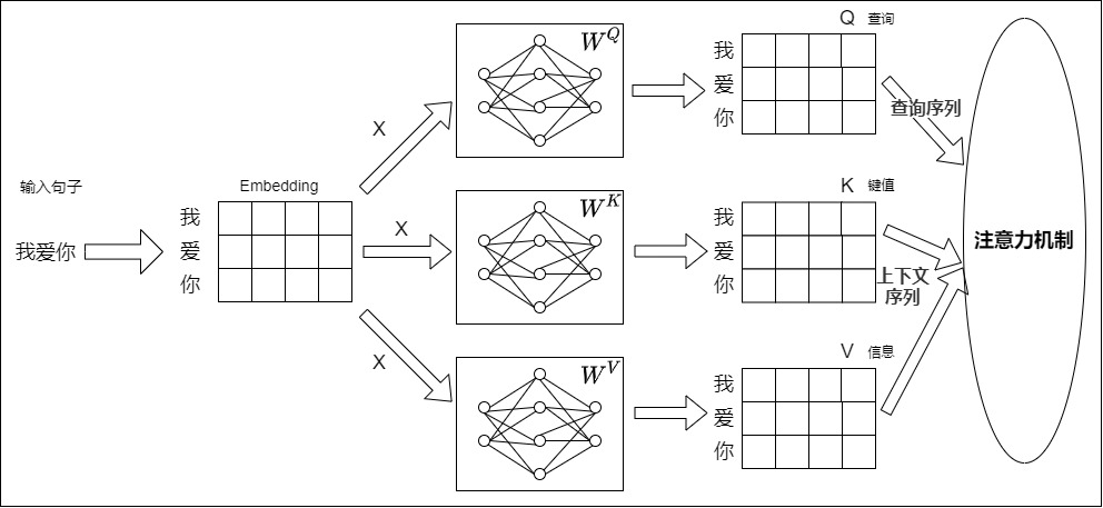
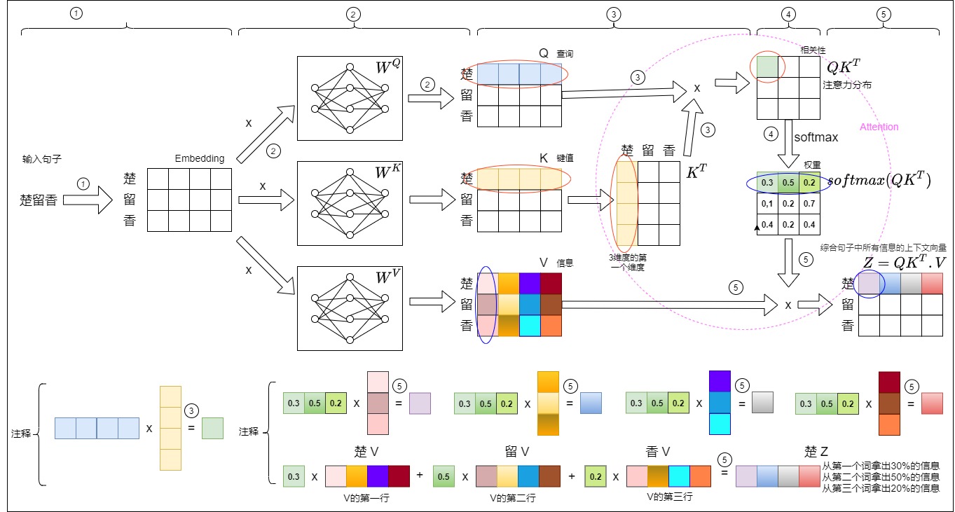
The source figure contains Chinese labels from the handwritten article. Read the three branches as learned role projections, not as three copies with fixed human meanings.
Worked detail Three readings of the query, key and value roles (soft database lookup, sequence alignment, value-space reconstruction) and where each one misleads; open it if the role names still feel arbitrary. (about 390 words, 3 code listings, 6 equations)
Three useful readings of the same Q/K/V contract
A10 approached Q/K/V from several directions. They are not competing definitions. Each highlights one invariant and becomes misleading when pushed too far.
Differentiable database reading
The database analogy makes the key-value pairing concrete:
query:
    a request represented in the learned matching space

key:
    an address or descriptor used to decide whether a slot is relevant

value:
    the payload retrieved if that slot receives weight
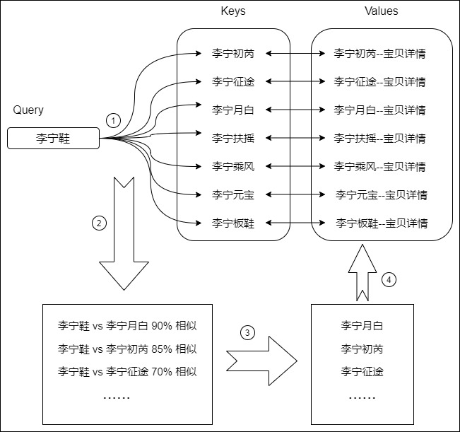
The source figure uses a shopping-query example and Chinese labels. Its useful claim is structural: candidate keys are scored first, and the values remain paired with those keys. Attention differs from a conventional database in at least four ways:
addresses are learned vectors rather than exact identifiers;
matching is dense similarity rather than equality;
the read normally mixes many values rather than returning one row;
the query, keys, values, and scoring projections train end to end.
The analogy therefore explains the read operation, not the storage engine. A Transformer attention layer does not sort scores, retrieve physical rows by ID, or necessarily materialize a top-k result. Dense attention evaluates every legal query-key pair and uses a differentiable weighted sum.
Sequence-to-sequence alignment reading
In encoder-decoder attention, the decoder state supplies a query while encoder states supply keys and values. Each target row obtains its own alignment over source positions:
The score row S[i,:] is target-indexed and source-normalized. This reading is
historically important because it connects Bahdanau/Luong alignment to the
Transformer primitive. It does not imply that every learned cross-attention
head is a clean lexical word-alignment model. Values may represent syntax,
position, discourse, or features that do not have one human label.
Contextual reconstruction reading
For self-attention, the output row is reconstructed from value rows:
This makes the operation a content-dependent linear combination in value
space. The coefficients are nonlinear functions of Q and K, so the complete
map from input states to output states is not linear. Conditional on a fixed
probability matrix P, however, the value path is linear:
That distinction matters for both interpretation and optimization. A heatmap shows the coefficients used for the current input. It does not show the value directions being moved, the output projection applied later, or the complete nonlinear function learned by the block.
The three readings agree on the contract:
Q/K decide where information is read from.
V decides what information crosses the selected edges.
The output remains indexed by queries.
They do not assign immutable semantics to vector coordinates. Query, key, and value are roles in one call, not permanent object types.
From one query to all query rows
For one query row, dot-product scores are:
Stack the memory keys as rows of matrix K. The complete score row becomes:
Now stack all queries as rows of Q:
The matrix multiplication is therefore not an arbitrary optimization applied
after defining attention. It is the batched form of every query comparing with
every available key. Row i, column j remains the pair (q_i, k_j).
0x03 Score matrix: QK^T / sqrt(d_k)
Before the Transformer, attention also used additive (Bahdanau) and bilinear, or “general” (Luong), score functions. The folded blocks below compare them; the visible text keeps the score computation, its shapes, and why the Transformer chose the scaled dot product.
The first real computation is:
d_k = query.size(-1)
scores = torch.matmul(query, key.transpose(-2, -1)) / math.sqrt(d_k)
Shape trace:
query:              [B, h, q_len, d_head]
key:                [B, h, k_len, d_head]
key.transpose:      [B, h, d_head, k_len]

scores:             [B, h, q_len, k_len]
The two middle sequence axes now have different meanings:
scores[..., i, j]
    = score for query row i against key row j
Rows are query positions. Columns are key/value positions.
This is one of the main objects later cost articles care about:
scores: [B, h, q_len, k_len]
When q_len = k_len = S, the score object is square: [B,h,S,S]. When cross-attention or decode changes the key axis, the object is not square. Treating all attention scores as [S,S] is a common source of bugs.
How this was checked How the score is split into compatibility, multiplier and finite bias for the rest of the article; open it if you want the exact notation behind later sections. (about 190 words, 2 equations)
Loop 3 contract: compatibility first, scaling second
Every attention family in this section must produce one scalar compatibility
for every legal query-key pair. Freeze the unscaled compatibility as u and
the multiplicative logit scale as alpha:
Here b is a finite preference such as position bias. Visibility is still the
separate boolean relation frozen in Loop 2. This ordering prevents three
different design choices from being hidden inside one word such as “score”:
| Contract field | Frozen meaning |
|---|---|
| compatibility family | the pair function f(q,k) before finite bias, visibility, or softmax |
logit multiplier alpha | inverse temperature applied to the compatibility |
temperature tau | tau = 1 / alpha when alpha > 0 |
| canonical Transformer choice | dot compatibility with alpha = Dk^(-1/2) |
| output contract | [B,Hq,Q,K], irrespective of how the pair function is evaluated |
Changing the family changes the model. Moving the same positive scalar between
algebraically equivalent locations should not change the real-number model,
although finite-precision execution can change. Loop 3 owns that distinction.
It does not own the complete softmax algorithm in 0x07, position-dependent
bias in M3.3, or context-length-dependent rescaling in M3.5.
Alternatives and history A table of score functions (dot, scaled dot, bilinear, additive, cosine) and why concatenation without a nonlinearity cannot rank keys; open it to compare the Transformer's choice with its predecessors. (about 230 words, 2 equations)
Alternative score functions and the Transformer choice
Scaled dot product is not the only differentiable compatibility function. The attention lineage used several choices:
| Score family | Mathematical and execution contract |
|---|---|
| dot product | u = q^T k; equal Q/K widths; no score-local parameters; all pairs are Q @ K^T |
| scaled dot product | s = alpha q^T k, canonically alpha = Dk^(-1/2); same pair program plus a fixed inverse temperature |
| bilinear / Luong general | u = q^T W_a k; Q/K widths may differ; W_a owns the cross-coordinate metric |
| additive / Bahdanau | u = v_a^T tanh(W_q q + W_k k + b_a); projected pair features and a nonlinear reduction |
| cosine / normalized QK | u = q_hat^T k_hat, optionally s = gamma u; norms are removed and the effective temperature is explicit |
A10 also lists the shorthand w^T[q;k] under concatenation similarity. Taken
literally without a nonlinearity, it is not an interactive additive score:
For one query row, w_q^T q is constant over every key. Row-wise softmax is
invariant to that constant, so the query-dependent term cancels. Bahdanau’s
additive score and Luong’s concat score insert a learned nonlinear hidden
layer; that hidden layer is what lets query and key jointly change the ranking.
The A10 shorthand is retained as source history, not as the implementation
contract.
Additive and multiplicative attention are legitimate design alternatives, not failed predecessors. The Transformer chose scaled dot product because projected queries and keys can be compared with a dense matrix multiplication, which is simple and accelerator-friendly, while the scale controls dimension-dependent logit growth. The choice couples an inductive assumption to a systems property: compatibility is represented by an inner product in a learned space, and all pairs can be evaluated by GEMM.
Alternatives and history Each score family derived from its assumption, with tensor shapes, parameter counts, one batched implementation and the limits of the Britz et al. comparison; open it when choosing or reimplementing a score function. (about 1,120 words, 5 code listings, 20 equations)
The alternatives also show what the projections are doing. A bilinear score
can absorb W_a into one side. Separate W_Q and W_K let the Transformer
learn two comparison spaces before the dot product. This does not make every
score family equivalent, but it makes scaled dot product much more expressive
than comparing raw input embeddings.
Deriving the score families from their interaction assumptions
The formulas look similar when reduced to a table, but they encode different pairwise interaction structures.
Dot product: coordinate agreement in a learned space
For q,k in R^d, the dot product is:
It rewards dimensions that have the same sign and large magnitude. Learned Q/K projections decide what those dimensions mean. There are no score-specific parameters after projection, and all query-key pairs become one GEMM:
This factorization constrains a single head’s unnormalized score matrix. If
Q in R^{Q_len x d_k} and K in R^{K_len x d_k}, then:
Softmax is nonlinear and value/output paths add capacity, so this is not a rank bound on the whole attention module. It is a precise property of the raw logit matrix.
The geometric decomposition separates angle from magnitude:
For fixed query i, its norm multiplies the entire score row and therefore
acts like a query-specific inverse temperature. A key norm changes one column
relative to other keys. The cosine term carries angular interaction. Calling a
dot product “only cosine similarity” drops two trainable magnitude channels.
Bilinear score: learn the interaction metric explicitly
Luong’s general score is:
If W_a is unconstrained, it can rotate, scale, and couple dimensions before
the comparison. In a Transformer with independent Q/K projections, part of
that freedom can be reparameterized into the projections:
This identity explains why a separate W_a is often unnecessary in the
scaled-dot-product design. It does not prove every bilinear parameterization
trains identically: initialization, sharing, dimensions, regularization, and
factorization rank differ.
For unequal widths Dq and Dk, choose
W_a in R^[Dq,Dk]. The batched tensor program is:
query:             [B,H,Q,Dq]
W_a:               [H,Dq,Dk]      # or shared [Dq,Dk]
query_metric:      [B,H,Q,Dk]
key:               [B,H,K,Dk]
score:              [B,H,Q,K]

query_metric = einsum("bhqd,hde->bhqe", query, W_a)
score        = query_metric @ key.transpose(-2, -1)
The score-local parameter count is H * Dq * Dk when every head owns a full
metric. Association order matters for work and temporary storage even though
(Q W_a)K^T = Q(W_a K^T) in exact arithmetic.
The following A10 figure rewrites projected dot-product attention as a learned
QK circuit. It is the bridge between Luong’s explicit bilinear metric and the
Transformer’s factorized W_Q W_K^T metric; the causal prefix shown in the
figure is one visibility policy, not part of the bilinear identity.
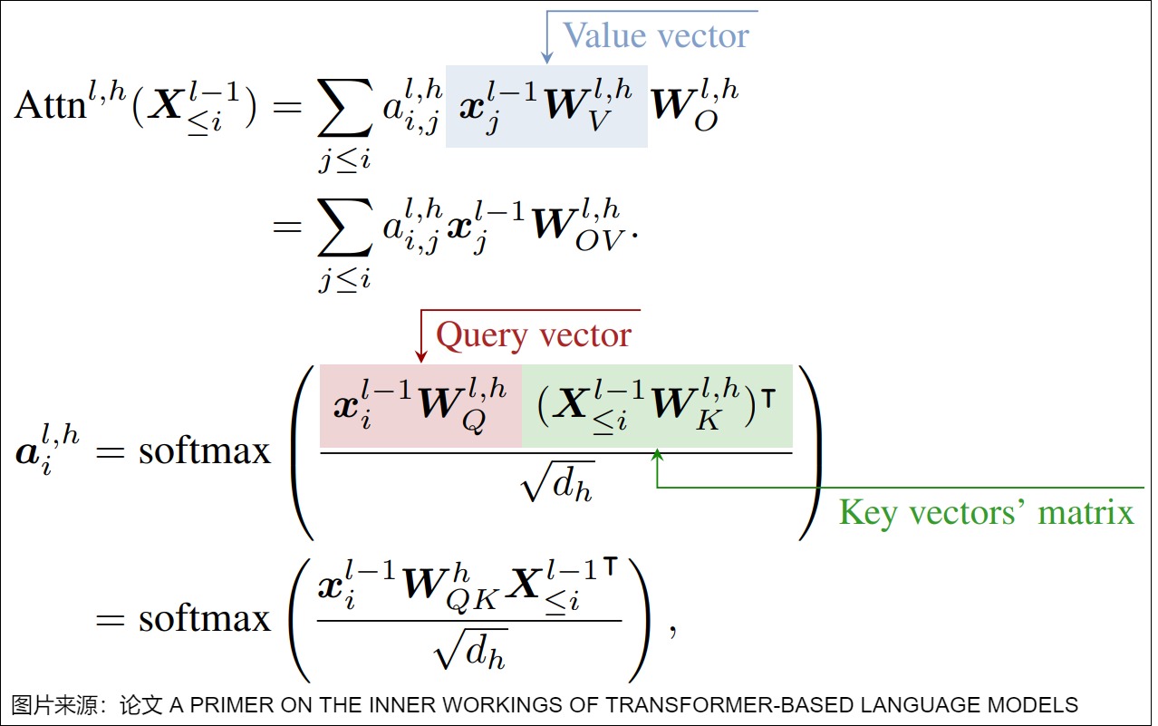
Visual provenance: reused from A10, where it is attributed to Ferrando et
al., A Primer on the Inner Workings of Transformer-based Language
Models. The semantic job here is the
factorization W_Q W_K^T, not an empirical claim.
Additive score: a learned nonlinear pair function
Bahdanau attention uses a small network:
For all pairs, projected query terms broadcast down the key axis and projected key terms broadcast across the query axis:
q_term: [B,Q,1,D_a]
k_term: [B,1,K,D_a]
pair:   [B,Q,K,D_a]
score:  [B,Q,K]
The nonlinear pair tensor gives additive attention a different interaction
family, but it also introduces a potentially large [B,Q,K,D_a] intermediate.
This is why “similar theoretical complexity” does not mean identical hardware
behavior. Dot-product attention maps its central pair operation directly onto
matrix multiplication.
With heads and unequal input widths, the full tensor trace is:
query:             [B,H,Q,Dq]
key:               [B,H,K,Dk]
W_q:               [H,Da,Dq]
W_k:               [H,Da,Dk]
v_a, b_a:          [H,Da]

q_term:            [B,H,Q,1,Da]
k_term:            [B,H,1,K,Da]
pair_hidden:       [B,H,Q,K,Da]
score:              [B,H,Q,K]
For independent per-head parameters, the score-local parameter count is:
where the final 2Da accounts for b_a and v_a. An implementation can tile
or fuse the pair operation instead of storing the complete five-dimensional
tensor, but it cannot silently replace the nonlinear pair function with GEMM
and still claim the same score family.
Cosine score: remove vector norm from compatibility
Cosine similarity with an explicit zero-norm policy is:
It bounds raw similarity to [-1,1] when norms are nonzero. A temperature or
learned scale is usually needed to give softmax an appropriate logit range.
Normalizing Q/K also changes the gradient: radial changes no longer affect the
score in the same way as angular changes.
The bounded interval is not automatically sharp enough. If one of K logits
is +1 and all others are -1, then without an extra multiplier the largest
possible probability is:
At K=128, this is only about 0.055. QKNorm is one concrete design point:
it L2-normalizes Q and K and replaces the fixed Dk^(-1/2) multiplier with a
learned scale. That is a changed model parameterization, not a different
placement of the canonical fixed scale.
One batched implementation oracle for all four families
The following pseudocode makes the common output axis and the family-specific temporary state explicit:
def compatibility(query, key, family, params, eps=1e-6):
    # query: [B,H,Q,Dq], key: [B,H,K,Dk]
    if family == "dot":
        assert query.shape[-1] == key.shape[-1]
        return query @ key.transpose(-2, -1)

    if family == "bilinear":
        # W: [H,Dq,Dk]
        q_metric = einsum("bhqd,hde->bhqe", query, params.W)
        return q_metric @ key.transpose(-2, -1)

    if family == "additive":
        # Wq: [H,Da,Dq], Wk: [H,Da,Dk], v/b: [H,Da]
        q_term = einsum("bhqd,had->bhqa", query, params.Wq)
        k_term = einsum("bhkd,had->bhka", key, params.Wk)
        pair = tanh(q_term[:, :, :, None, :]
                    + k_term[:, :, None, :, :]
                    + params.b[None, :, None, None, :])
        return einsum("bhqka,ha->bhqk", pair, params.v)

    if family == "cosine":
        assert query.shape[-1] == key.shape[-1]
        q_hat = query / norm(query, dim=-1, keepdim=True).clamp_min(eps)
        k_hat = key / norm(key, dim=-1, keepdim=True).clamp_min(eps)
        return q_hat @ k_hat.transpose(-2, -1)

    raise ValueError(f"unknown score family: {family}")
Only the dot-family result can be handed directly to the canonical SDPA primitive. Bilinear may be reducible to transformed Q or K before SDPA. Additive requires a different score kernel or an explicit pair program. Cosine requires normalization and, usually, an explicit scale. Backend availability is therefore part of the design choice, not an afterthought.
What the historical comparison does and does not establish
A10 reused the following table from Britz et al.’s large NMT architecture
study. It is useful evidence that additive and multiplicative families can be
competitive under a matched recurrent NMT experiment. It is not a universal
ranking of Transformer attention mechanisms, and the Mul rows are not the
canonical scaled Transformer primitive.
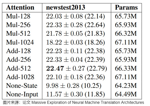
Visual provenance: A10 attributes this table to Britz et al., Massive Exploration of Neural Machine Translation Architectures. The table is source-reported, task-specific evidence. State width, recurrent architecture, training recipe, and measurement uncertainty prevent a general winner claim.
The implementation choice is therefore not just “which formula has fewer symbols.” It chooses:
the pairwise function class;
where trainable parameters live;
which pair tensors are materialized;
which operation accelerators execute efficiently;
how logit magnitude is controlled.
For M3.1, scaled dot product remains the reference because it is the model contract used by the canonical Transformer path. The alternatives are retained to explain the design space, not treated as interchangeable aliases.
0x04 Why the scale exists
The original Transformer defines scaled dot-product attention as:
The division by sqrt(d_k) is not decoration.
If the query and key components are roughly independent with unit variance, then a dot product sums d_k products. The variance of the unscaled dot product grows with d_k, and the standard deviation grows like:
Large-magnitude logits push softmax toward saturation:
one score dominates
other probabilities approach zero
gradients through softmax shrink
Scaling by sqrt(d_k) keeps the logit scale less sensitive to the head dimension. In per-head attention, the scale is the per-head width:
d_k = query.size(-1) # d_head, not d_model
Using d_model here when query is already split into heads returns a tensor with the same shape and the wrong temperature.
Variance derivation, assumptions, and temperature interpretation
First freeze the notation. Frameworks often call alpha a scale, while
statistical mechanics and sampling discussions usually name its reciprocal the
temperature:
The canonical Transformer chooses:
This article uses multiplier for alpha and temperature for tau.
Otherwise phrases such as “increase the scale” are ambiguous: increasing
alpha sharpens logits, while increasing tau flattens them.
Let one unscaled logit be:
Assume for the initialization argument that components are independent across
r, that q_r and k_r have mean zero, and that both have variance one. Then:
Also:
The variance of the sum is therefore:
and its standard deviation is sqrt(d_k). Dividing produces:
Derivation The variance result for general means and covariances, and why dependent Q and K need more than second moments; open it if you doubt the unit-variance assumption. (about 230 words, 6 equations)
The unit-variance case is only the shortest corollary. Suppose instead that Q
and K are independent random vectors with means mu_q, mu_k and covariance
matrices Sigma_q, Sigma_k. Then:
and:
For zero means this reduces to
tr(Sigma_q Sigma_k). If coordinates are isotropic with variances
sigma_q^2 and sigma_k^2, it becomes:
so the canonical multiplier leaves variance
sigma_q^2 sigma_k^2, not necessarily one. The fixed 1/sqrt(d_k) term
removes dimension-driven growth; it does not normalize arbitrary learned Q/K
statistics.
If Q and K are statistically dependent, second moments alone generally do not determine the variance of their product sum. One needs cross moments or a stronger distributional assumption. This matters in self-attention because Q and K can originate from the same residual state. The Transformer footnote is an initialization-scale argument under independence, not a theorem about every trained logit distribution.
The assumptions are an initialization-scale explanation, not a claim that
trained Q/K components remain independent standard-normal variables. Learned
projections, normalization, position mechanisms, and data create correlations.
The fixed scale still removes the most direct dimensional growth from summing
d_k products.
From logit spread to a small softmax Jacobian
The original Transformer paper motivates scaling by the small gradients of
softmax when unscaled dot products become large. The local statement can be
made exact. For one row p = softmax(s), the Jacobian is:
If one logit exceeds all others by gaps that tend to infinity, p approaches
a one-hot vector. Every entry of diag(p)-pp^T then approaches zero. Thus an
upstream gradient reaching the probability row is strongly attenuated through
the score path. This is a local Jacobian statement, not a promise that every
parameter gradient in the complete residual network vanishes.
For two logits with gap Delta, the winning probability is logistic:
and its local derivative with respect to the scaled gap is:
Increasing the multiplier alpha sends a fixed nonzero gap toward a hard
decision and sends this derivative toward zero. This is the precise bridge
from dimension-dependent logit variance to softmax saturation. 0x07 later
owns the complete row-wise softmax and backward contracts.
Softmax can be written with temperature tau:
Larger tau produces a flatter distribution; smaller tau produces a sharper
one. The Transformer uses tau=sqrt(d_k). Accidentally scaling by sqrt(d_model)
when d_model=h*d_k makes the temperature larger by sqrt(h), flattening
attention relative to the intended per-head equation.
For d_model=4096 and h=32:
d_head = 128
correct divisor: sqrt(128)  ~= 11.31
wrong divisor:   sqrt(4096) = 64
temperature ratio:          ~= 5.66
The error is numerically large and shape-invisible.
How this was checked Expected results of a numerical sweep over head widths 8, 32 and 128 that confirms the variance formula; open it to see how a missing or wrong scale shows up. (about 90 words)
An executable reference sweep in the Loop 3 evidence package samples independent standard-normal Q/K components. Its expected ledger is:
| Width and quantity | Expected behavior |
|---|---|
raw variance at d_k = 8, 32, 128 | grows approximately as 8, 32, 128 |
scaled variance with alpha = d_k^(-1/2) | stays approximately 1 |
standard deviation ratio, raw 128 vs raw 8 | approximately sqrt(128/8) = 4 |
wrong d_model divisor for 32 heads | multiplier is too small by sqrt(32) ~= 5.66 |
Sampling error is expected; the analytic formula is the contract. The sweep is a diagnostic that catches an omitted scale, the wrong dimension, or accidental double scaling.
Implementation and runtime contracts Where the scale may be applied (after the product, on Q, on K, or split as d_k^(-1/4) on each side) and how PyTorch's scale argument avoids scaling twice; open it when porting a checkpoint or calling a fused kernel. (about 220 words, 3 code listings)
Scale placement and fused APIs
Let alpha > 0 be the effective logit multiplier. These four placements are
algebraically equivalent in exact arithmetic:
scores_post = (q @ k.transpose(-2, -1)) * alpha

scores_q = (q * alpha) @ k.transpose(-2, -1)

scores_k = q @ (k * alpha).transpose(-2, -1)

root_alpha = math.sqrt(alpha)
scores_split = (q * root_alpha) @ (k * root_alpha).transpose(-2, -1)
For canonical attention, alpha = d_k^(-1/2). The symmetric multiplier on
each operand is therefore sqrt(alpha) = d_k^(-1/4), a detail that is easy to
get wrong. Scaling both Q and K by d_k^(-1/2) applies an effective multiplier
of d_k^(-1) and changes the model.
The placements are not bitwise equivalent in finite precision. Pre-scaling Q
or K rounds the operands before accumulation. Post-scaling rounds the
dot-product accumulator. A fused kernel may fold the multiplier into a tiled
score/softmax pipeline without ever materializing scores. Parity should
therefore compare outputs and gradients under a declared tolerance, while the
immutable contract compares the effective real-number multiplier.
PyTorch 2.13’s functional SDPA contract names this multiplier scale:
alpha = d_k ** -0.5

# Canonical default: the API derives alpha from query.size(-1).
out_default = F.scaled_dot_product_attention(q, k, v, scale=None)

# Explicit checkpoint or model contract.
out_explicit = F.scaled_dot_product_attention(q, k, v, scale=alpha)
The keyword is applied before softmax. It is a multiplier, not the denominator
temperature. If Q is already pre-scaled by alpha, preserve that model with
scale=1.0; leaving scale=None would apply the default multiplier again:
# Correct only when q_scaled already contains the complete alpha.
out = F.scaled_dot_product_attention(q_scaled, k, v, scale=1.0)

# Wrong: effective multiplier becomes alpha * d_k**(-0.5).
out_double_scaled = F.scaled_dot_product_attention(q_scaled, k, v)
The backend may differ while this semantic multiplier remains fixed.
Conversely, changing from the canonical multiplier to a learned per-head
gamma, a length-dependent multiplier, or a score soft-cap is a model change
even if the same kernel can execute it. M3.5 owns context-extension scaling;
M4 owns whether a requested placement/backend is actually faster.
How this was checked An eager-versus-fused comparison that catches shape-preserving scale errors (d_model instead of d_k, scaling twice, a multiplier read as a denominator); open it when testing a new backend. (about 50 words, 1 code listing)
Scale-placement validation gate
Before comparing eager and fused results, record and assert:
assert manifest.compatibility_family == "dot"
assert manifest.scale_semantics == "multiplicative_inverse_temperature"
assert manifest.effective_logit_multiplier == configured_alpha
assert manifest.scale_application_count == 1
assert manifest.scale_width == query.shape[-1]  # unless checkpoint overrides it

eager_scores = (q @ k.transpose(-2, -1)) * configured_alpha
eager_out = softmax(eager_scores + bias_or_mask, dim=-1) @ v

fused_out = F.scaled_dot_product_attention(
    q, k, v,
    attn_mask=bias_or_mask,
    dropout_p=0.0,
    scale=configured_alpha,
)

assert_close(eager_out, fused_out, atol=declared_atol, rtol=declared_rtol)
This gate catches the dangerous failures that preserve every tensor shape:
using d_model instead of d_k, applying the multiplier twice, interpreting
an inverse temperature as a denominator, or comparing two backends under
different configured scales.
0x05 Optional finite bias: inherited score preferences
M3.3 opens the relative-position score tensor and shows that some mechanisms add finite score preferences before softmax:
scores = scores + position_bias
M3.1 only needs the slot:
if position_bias is not None:
    scores = scores + position_bias
Typical compatible shapes:
scores:        [B, h, q_len, k_len]

position_bias: [1, h, q_len, k_len]
position_bias: [B, h, q_len, k_len]
position_bias: [q_len, k_len]       # if intentionally shared
The semantic contract is:
position_bias:
    finite preference among keys that may be visible

attention_mask:
    visibility / illegality
A finite bias can encourage or discourage a key. It cannot make a future key legal. It cannot make a PAD key meaningful. That is why the mask remains authoritative.
How this was checked The masked softmax written as an equation over legal keys only, why a large finite negative constant only approximates it, and which earlier stage builds each mask input; open it for the exact definition of masking used throughout. (about 430 words, 8 equations)
Loop 4 contract: one support relation, several physical encodings
Freeze the pre-softmax row in three layers:
followed by a Boolean visibility predicate . The model-level probability is not merely “softmax plus a mask.” It is softmax on a restricted support:
This equation fixes four properties before selecting an API:
- each query row has its own legal key set;
- an illegal key is absent from both numerator and denominator;
- finite bias changes probability ratios within the legal set;
- visibility changes the support itself.
The familiar additive representation is one implementation of the same extended-real contract:
Using a large finite negative constant only approximates this support rule. If
one illegal entry has original logit z_bad, receives additive penalty -C,
and the legal row denominator is Z_legal, then it still receives
in exact arithmetic. Whether it rounds to zero depends on score range,
accumulation dtype, and backend. -inf expresses illegality; -1e9 is a
historical implementation sentinel whose behavior must be tested in the
actual dtype.
Construction owner versus application owner
M3.1 does not invent document boundaries or decide which labels train. It consumes a structured batch contract and applies the resulting relation at the score boundary:
| Object | Constructed by | Consumed here as | Deferred concern |
|---|---|---|---|
| token validity, lengths, padding side | M2.1 | legal key columns and query-valid rows | tokenizer/collator policy |
| segment IDs or cumulative lengths | M2.1 | same-segment visibility or varlen metadata | pack assignment and label boundaries |
| target shift and objective topology | M3.9 | causal, prefix, or other declared support | supervised-row ownership |
| positional geometry and request-local cache frontier | M3.3, M3.4, and M3.5 construct positional geometry; M3.10 supplies the request-local cache-position/frontier relation | query/key coordinates in the predicate | persistent cache publication, physical mutation, and rollback in M5.1 and M5.3 |
visible[b,h,i,j] | M3.1 | exclusion before row normalization | optimized IO schedule in M4.3 |
The boundary is deliberate. M2.1 can prove that token j belongs to document
d; M3.9 can prove that output row i predicts a particular target; M3.1
proves whether score edge (i,j) participates in the denominator.
This article does not re-explain T5 buckets, Shaw relative vectors, ALiBi slopes, DeBERTa, TUPE, RoPE, or length extrapolation. Those belong to M3.3, M3.4, and M3.5.
0x06 Visibility mask before softmax
Masks come in many forms, so this section is long. The visible text keeps the rule (an illegal key is removed before softmax, so it is absent from both the numerator and the denominator of its row; the text calls this restricted-support softmax, and its equation is in the last folded block of 0x05), the causal and padding cases, how they combine, and why every used query needs at least one legal key. The folded blocks cover cached-decoding alignment, mask polarity in different APIs, unused query rows, packing, prefix and window designs, and how masks are built and handed to fused kernels.
The Harvard attention code applies the mask after score construction and before softmax:
if mask is not None:
    scores = scores.masked_fill(mask == 0, -1e9)

p_attn = scores.softmax(dim=-1)
Conceptually, use -inf:
scores = scores.masked_fill(mask == 0, -float("inf"))
The role of the mask is not to nudge a preference. It removes illegal key positions from the softmax distribution.
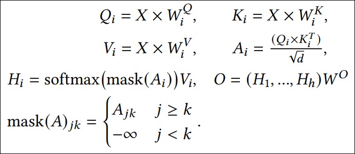
Masking is exclusion, not multiplication or post-softmax erasure
Three shape-compatible programs are often described as “apply the mask,” but only one directly implements restricted-support softmax.
# Correct hard exclusion before normalization.
masked_logits = logits.masked_fill(~visible, -torch.inf)
probabilities = torch.softmax(masked_logits, dim=-1)

# Wrong: an illegal score becomes zero, and exp(0) is positive.
multiplied_logits = logits * visible
probabilities = torch.softmax(multiplied_logits, dim=-1)

# Wrong unless followed by an explicit renormalization over legal entries.
probabilities = torch.softmax(logits, dim=-1)
probabilities = probabilities * visible
For the last program, if p = softmax(logits) and at least one legal entry
exists, then
recovers the same exact distribution as pre-softmax exclusion. Merely zeroing entries does not: the remaining row sums to less than one, and the illegal logits already affected the original denominator. Pre-softmax exclusion is therefore both the simpler contract and the form fused attention APIs expect.
The A11 prose sometimes says “multiply by a mask” while its executable Harvard
code uses masked_fill before softmax. Treat the code path and the
restricted-support equation as authoritative; literal multiplication by a
zero-one matrix is not equivalent.
Causal mask
In decoder self-attention, query row i should not read future key rows j > i.
visible(i, j) = j <= i
For a length-5 prefix:
query\key   0  1  2  3  4
0           1  0  0  0  0
1           1  1  0  0  0
2           1  1  1  0  0
3           1  1  1  1  0
4           1  1  1  1  1
That lower triangle is only the square, zero-offset special case. The general causal predicate compares absolute positions:
This form survives left padding, rectangular cross-shapes, chunked decoding, and static caches because legality is attached to coordinates rather than matrix corners.
Edge cases and failure behaviour Why a "lower-triangular" mask is ambiguous when there are fewer queries than keys, as in cached decoding, and how absolute positions and PyTorch's is_causal alignment settle it; open it before decoding with a cache. (about 210 words, 3 code listings)
Rectangular causal alignment is part of the contract
For Q=2, K=5, the phrase “lower triangular” is ambiguous. Upper-left
alignment produces:
q\k  0 1 2 3 4
 0   1 0 0 0 0
 1   1 1 0 0 0
This is correct when the two query rows have absolute positions [0,1]. It is
wrong for a decode chunk representing absolute positions [3,4], which needs
lower-right alignment:
q_abs\k_abs  0 1 2 3 4
      3      1 1 1 1 0
      4      1 1 1 1 1
The second relation follows from coordinates, not from a special drawing:
q_pos = torch.arange(q_len, device=device) + past_len
k_pos = torch.arange(k_len, device=device)
visible = k_pos[None, :] <= q_pos[:, None]
PyTorch 2.13 documents that scaled_dot_product_attention(..., is_causal=True) uses an upper-left causal bias for non-square matrices.
Its prototype CausalBias API distinguishes causal_upper_left from
causal_lower_right. Consequently, is_causal=True is not a generic promise
that an arbitrary cache offset will be inferred. A runtime must prove that the
API’s alignment matches its query/key coordinates, or pass an explicit bias
that does.
| Call shape | Query coordinates | Key coordinates | Dense support |
|---|---|---|---|
square prefill Q=K=T | 0..T-1 | 0..T-1 | ordinary lower triangle |
| one-token contiguous decode | [past_len] | 0..past_len | one fully legal row |
chunk decode Q=c, K=past+c | past..past+c-1 | 0..past+c-1 | lower-right triangle |
static cache K=capacity | current absolute rows | slot positions plus validity | causal AND initialized-slot validity |
The table separates semantic causality from physical extent. A cache tensor can contain allocated but uninitialized slots; no triangle can infer those slots are invalid from shape alone.
The mask prevents future-token leakage inside attention. Target shifting and loss alignment are separate training objects owned by M3.9.
Padding mask
Padding keys should not receive probability mass.
For source padding, a typical key mask is:
src_key_visible: [B, 1, 1, S]
The 1 axes broadcast across heads and query rows:
scores:          [B, h, q_len, S]
src_key_visible: [B, 1,     1, S]
Padding masks primarily hide key/value columns. If a query row itself is padding, downstream training loss or pooling code must also avoid treating that row as meaningful. That is not solved by letting the row attend to nothing.
A11’s padding illustration is useful precisely because it exposes this distinction:
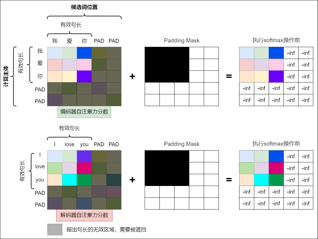
Edge cases and failure behaviour Why masking padded query rows as well as padded key columns leaves rows with no legal key, and why key validity and query validity are separate tensors; open it when your batches pad queries. (about 130 words, 1 code listing, 2 equations)
Read the rightmost matrix critically. Masking PAD columns excludes
meaningless K/V rows from every query denominator. Masking the PAD query
rows as well creates rows containing only -inf; ordinary softmax does not
turn those rows into a mathematically defined row of zeros. A real
implementation therefore needs two objects:
key_valid[b,j]:
    may key/value row j contribute to any query?

query_valid[b,i]:
    will output row i be consumed by residual, pooling, or loss code?
Query validity and key validity are different tensors. In particular,
query_valid is separate from the relation normalized by attention; it may
govern output zeroing or downstream loss without deleting every key from that
physical query row.
For a padded encoder batch, the attention relation can remain
while query_valid separately zeros or ignores outputs at synthetic query
rows. Conflating these objects is how an apparently reasonable two-dimensional
padding picture becomes an all-masked-row bug.
Combined target mask
A decoder target mask often combines padding visibility and causal visibility:
target_pad:      [B, 1, T]
causal:          [1, T, T]

combined:        [B, T, T]
score-ready:     [B, 1, T, T]
The exact rank differs by implementation. The invariant is that the final mask must broadcast to:
scores: [B, h, q_len, k_len]
Implementation and runtime contracts The opposite meanings of True in Harvard code, PyTorch SDPA, nn.MultiheadAttention and additive masks, adapters between them, and the mask shapes each API expects; open it before passing a mask to a library. (about 200 words, 3 code listings)
Boolean and additive conventions
The dangerous part is not the mask idea. It is API polarity.
| Convention | Allowed position | Blocked position | Operation |
|---|---|---|---|
| Harvard-style boolean | 1 / True | 0 / False | masked_fill(mask == 0, -inf) |
PyTorch SDPA boolean attn_mask | True participates | False blocked | blocked entries receive -inf bias |
PyTorch MultiheadAttention binary attn_mask | False allowed | True not allowed | API interprets True as blocked |
PyTorch MultiheadAttention key_padding_mask | False token kept | True token ignored | padding-side mask convention |
| Additive float mask | 0.0 | -inf or very negative | added to scores |
Same dtype, opposite polarity is a silent correctness bug.
Do not let an untyped tensor named mask cross the model/backend boundary.
Convert from one canonical semantic object in a named adapter:
def visible_to_sdpa_bool(visible):
    # SDPA: True participates.
    return visible.bool()

def visible_to_mha_attn_mask(visible):
    # MultiheadAttention binary attn_mask: True is blocked.
    return ~visible.bool()

def key_valid_to_mha_padding_mask(key_valid):
    # MultiheadAttention key_padding_mask: True is ignored.
    return ~key_valid.bool()

def visible_to_additive_bias(visible, dtype):
    bias = torch.zeros(visible.shape, dtype=dtype, device=visible.device)
    return bias.masked_fill(~visible, -torch.inf)
PyTorch’s public contracts also differ in rank:
SDPA attn_mask:
    broadcastable to [B,...,Hq,Q,K]

MultiheadAttention attn_mask:
    [Q,K] or [B*H,Q,K]

MultiheadAttention key_padding_mask:
    [B,K]
If MultiheadAttention receives both attn_mask and key_padding_mask, its
documentation requires their types to match. The module expands and merges
them internally. That convenience does not erase the semantic distinction:
attn_mask represents query-key edges, while key_padding_mask represents
key-column validity.
Float masks add values rather than declare a Boolean support. They must match the API’s required dtype and device, and any finite entries are preferences, not authoritative exclusion. A release manifest should therefore record:
canonical polarity: True = visible
adapter/API: SDPA bool | MHA blocked bool | additive float | block metadata
materialized shape and broadcast axes
causal alignment: square | upper-left | lower-right | explicit positions
all-masked-row precondition or policy
All-masked rows
One more failure is easy to miss:
scores[i, :] = [-inf, -inf, -inf, ...]
Softmax over an all-masked row can produce NaN, because there is no legal key for that query. This can happen with malformed padding, empty cross-attention memory, or a bad combination of causal and padding masks.
The reason is structural, not an arbitrary library limitation. Restricted softmax would require
but the legal set is empty, so both the intended numerator and denominator vanish. There is no probability distribution over an empty support.
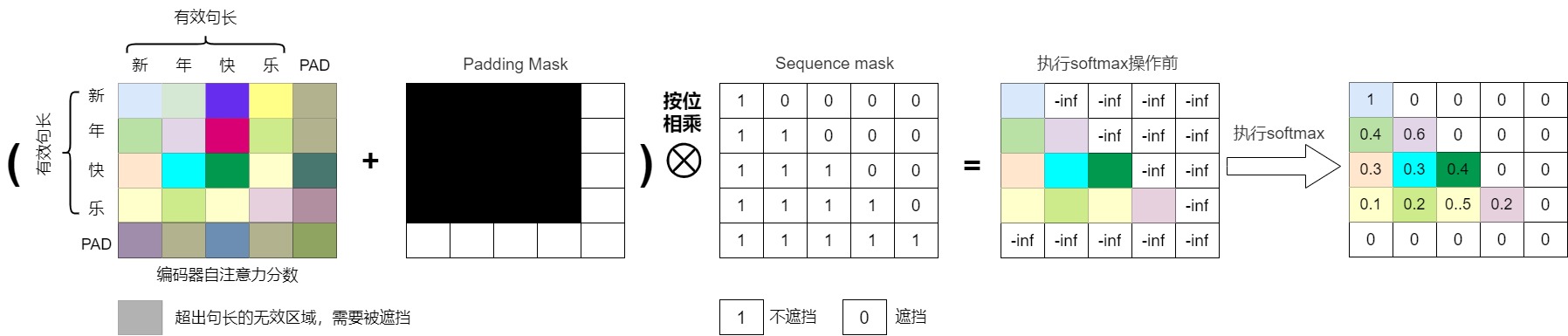
The A11 figure labels the final PAD query row as zeros after softmax. That is a
useful desired output policy, but it does not follow from applying ordinary
softmax to five -inf logits. The implementation must explicitly reject the
row, give it a sentinel legal key, or mark it unused and zero its output. The
figure must not be read as a numerical derivation.
The mask contract is not just “make illegal logits small.” It is:
Every query row that will be used must have at least one legal key.
Edge cases and failure behaviour Three policies for query rows whose outputs are never used (reject them, give them a sentinel key, or mark them and zero their outputs), a reference implementation, and why zeroing NaN afterwards is weaker; open it when batches contain padded queries. (about 230 words, 4 code listings)
Policies for structurally unused query rows
Some batches contain query rows whose outputs will never be consumed, such as PAD query positions. There are three defensible policies, but they must not be mixed implicitly.
Policy 1: reject all-masked rows.
This is the strongest reference behavior:
assert visible.any(dim=-1).all()
It catches malformed examples early and is appropriate when every query row is expected to represent a real token.
Policy 2: give every physical query a legal sentinel key.
A dedicated null/sentinel slot can make the row mathematically defined. The sentinel value and its downstream treatment become learned/model state; this is not equivalent to pretending the row did not exist.
Policy 3: mark unused queries separately and zero their outputs.
Here key visibility and query validity are different tensors:
key_visible = ...   # [B,1,Q,K], relation used by softmax
query_valid = ...   # [B,1,Q,1], whether output row is consumed
A safe reference implementation can temporarily make one key legal for unused queries, normalize, then zero the output:
def attention_with_unused_queries(q, k, v, visible, query_valid):
    visible = torch.broadcast_to(visible, (*q.shape[:-1], k.size(-2)))
    query_valid = torch.broadcast_to(query_valid, (*q.shape[:-1], 1))

    no_key = ~visible.any(dim=-1, keepdim=True)
    assert torch.all(~(no_key & query_valid))

    safe_visible = visible.clone()
    safe_visible[..., 0:1] |= no_key

    scores = (q @ k.transpose(-2, -1)) * (q.size(-1) ** -0.5)
    scores = scores.masked_fill(~safe_visible, -torch.inf)
    probabilities = torch.softmax(scores, dim=-1, dtype=torch.float32)
    output = probabilities.to(q.dtype) @ v

    output = output * query_valid.to(output.dtype)
    return output
The temporary key is an implementation device for unused rows only. It must never make a real query legal when its semantic key set is empty.
Zeroing NaN after an undefined softmax is weaker:
probabilities = torch.nan_to_num(softmax(all_negative_infinity_row))
That can hide a real visibility bug and gives backend-dependent gradients. Choosing a policy before normalization makes forward and backward behavior auditable.
Optimized kernels may define their own all-masked-row result. A backend parity test must include this case explicitly or exclude it by precondition; it should not discover the policy accidentally in production.
Code and tensors Small functions that build causal and padding visibility apart from the single line that applies it; open it when writing mask code or locating a mask bug. (about 90 words, 3 code listings)
Mask construction and mask application are different interfaces
The attention kernel should not have to infer why an entry is illegal. Upstream code constructs visibility from semantic objects; the score path only applies the resulting rule.
def make_causal_visibility(q_len, k_len, past_len=0, device=None):
    q_pos = torch.arange(q_len, device=device) + past_len
    k_pos = torch.arange(k_len, device=device)
    return k_pos[None, :] <= q_pos[:, None]       # [q_len, k_len]

def make_key_padding_visibility(attention_mask):
    # attention_mask: [B, k_len], 1 means a real token.
    return attention_mask[:, None, None, :].bool()  # [B,1,1,k_len]

def combine_visibility(causal, key_visible):
    return causal[None, None, :, :] & key_visible
Application then has one narrow contract:
visible = combine_visibility(causal, key_visible)  # broadcastable to scores
masked_scores = scores.masked_fill(~visible, -torch.inf)
Separating the interfaces makes failures easier to localize:
wrong legal positions:
    construction bug

right legal positions, wrong polarity or dtype:
    application/API bug

right mask, NaN row:
    no legal key or unstable backend path
The distinction also matters for cached decoding. With q_len=1, the causal
row must use the absolute query position, not local row zero. Otherwise a
current token at absolute position 127 would be allowed to read only key zero.
Worked detail Visibility written as predicates for packed samples (block-diagonal, with pair counts for lengths 3, 4, 5 and 4), encoder, decoder, cross-attention and cached decoding, plus prefix-LM and sliding-window designs; open it for masks beyond causal and padding. (about 680 words, 3 code listings, 20 equations)
Packed samples require block-diagonal visibility
Packing several independent examples into one physical token row removes PAD tokens, but it does not make the examples one sequence. A causal mask alone would let a token in the second example read tokens from the first example.
For packed segment IDs:
segment: [0,0,0, 1,1,1,1, 2,2, 3,3,3]
position:[0,1,2, 0,1,2,3, 0,1, 0,1,2]
legal visibility is the conjunction:
same_segment = segment_ids[:, None] == segment_ids[None, :]
causal_local = positions[:, None] >= positions[None, :]
packed_visible = same_segment & causal_local
Packing changes the physical schedule, not the independent-example semantics.
For lengths l_1,...,l_n, padding every example to L=max(l_s) presents
nL token slots and up to
query-key score pairs to a dense batched kernel. Independent variable-length execution needs only
dense pairs before causal triangular savings. Concatenating all tokens and running one unrestricted dense matrix would instead expose
including cross-document pairs that must not exist. Block-diagonal visibility recovers the independent semantics; a varlen kernel can also avoid materializing or computing the off-block region.
For A11’s lengths [3,4,5,4]:
padded dense pairs:       4 * 5^2 = 100
independent dense pairs:  3^2 + 4^2 + 5^2 + 4^2 = 66
unrestricted concat:     16^2 = 256   # wrong support and extra work
These are logical pair counts, not a claim that every backend materializes the score matrix. M4.3 owns the IO schedule and kernel-level traffic.
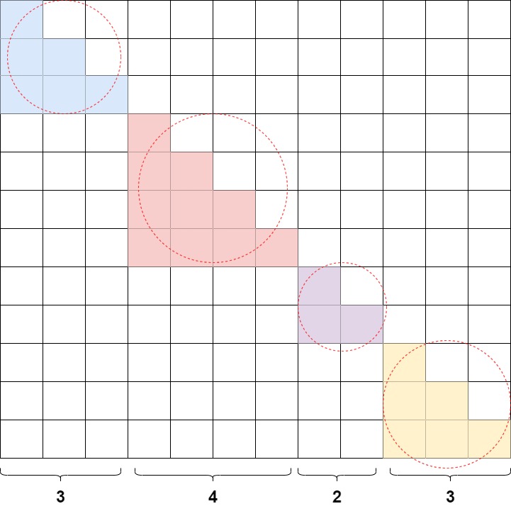
The source visual marks each packed sample as its own causal triangle. This is the semantic requirement. A production kernel may represent the same structure with cumulative sequence lengths and avoid materializing the dense mask.
Mask algebra across encoder, decoder, cross-attention, and cache modes
Write visibility as predicates rather than pictures. Let query position be i,
key position be j, batch row be b, and real[b,j] indicate a non-padding
key.
The omitted head index is intentional only when every head shares topology.
The full object is V[B,H,Q,K]; a physical [Q,K], [B,1,Q,K], or
[B,1,1,K] tensor is valid only because its omitted axes are declared
broadcast-invariant. Head-specific windows or sparsity require an H axis and
must not be silently collapsed to one shared mask.
Encoder self-attention normally uses:
Every real query can read every real key. Query padding still needs a separate downstream contract because key masking only controls which values enter a row.
Decoder causal self-attention uses:
Cross-attention from target query i to source key j uses:
unless the application adds an explicit source-memory restriction. There is no generic target causal triangle on the source axis. The target row is already conditioned on legal target history before it queries source memory.
For cached decoding, use absolute positions. Let the current query positions be
p_i and cached key positions be r_j:
If the implementation appends exactly one current key after a contiguous past, all provided keys satisfy the predicate and an explicit triangular mask may be redundant. That does not justify removing masks from every decode kernel. Chunked decode, speculative branches, static cache buffers, left padding, and mixed-length batches can expose keys whose validity cannot be inferred from tensor extent alone.
Prefix and window masks are visibility designs, not score biases
A prefix language model may allow all prefix rows to see one another while continuation rows are causal:
A causal sliding window of width w uses:
These masks remove edges from the attention graph. A finite position bias does
not: a sufficiently strong content score can overcome a finite negative bias,
while a masked edge must remain impossible. That is why ALiBi-like preferences,
relative-position biases, prefix visibility, and sliding-window legality should
not all be represented by an undocumented float tensor called mask.
Implementation and runtime contracts How a visibility relation is compiled, composed and encoded for backends (dense, additive, sequence lengths, block masks), where masks arise in training and inference pipelines, and the rules for packed batches with a test; open it when building a data or serving pipeline. (about 1,500 words, 16 code listings)
One predicate compiler, not one universal dense matrix
A transparent reference compiler can combine declared semantic inputs before choosing a physical encoding:
def compile_visibility(
    q_pos,                 # [B,Q] absolute or segment-local coordinates
    k_pos,                 # [B,K]
    key_valid,             # [B,K]
    *,
    causal=False,
    q_segment=None,        # [B,Q]
    k_segment=None,        # [B,K]
    prefix_length=None,    # scalar or [B]
    window=None,
):
    visible = key_valid[:, None, :]          # [B,1,K]

    if q_segment is not None or k_segment is not None:
        assert q_segment is not None and k_segment is not None
        visible = visible & (
            q_segment[:, :, None] == k_segment[:, None, :]
        )

    if prefix_length is not None:
        P = torch.as_tensor(prefix_length, device=q_pos.device)
        if P.ndim == 0:
            P = P.expand(q_pos.size(0))
        q_in_prefix = q_pos < P[:, None]
        k_in_prefix = k_pos < P[:, None]
        topology = (
            (q_in_prefix[:, :, None] & k_in_prefix[:, None, :])
            | (~q_in_prefix[:, :, None]
               & (k_pos[:, None, :] <= q_pos[:, :, None]))
        )
        visible = visible & topology
    elif causal:
        visible = visible & (
            k_pos[:, None, :] <= q_pos[:, :, None]
        )

    if window is not None:
        distance = q_pos[:, :, None] - k_pos[:, None, :]
        visible = visible & (distance >= 0) & (distance < window)

    return visible[:, None, :, :]            # [B,1,Q,K]
This is an eager semantic oracle, not a recommendation to materialize a
dense mask at long sequence lengths. A production adapter may lower the same
predicate to an is_causal flag, sequence lengths, cumulative offsets,
CausalBias, or block metadata. The lowering is correct only if it preserves
every (b,h,i,j) truth value.
The function also exposes incompatible requests. A prefix topology already
defines its own causal region; blindly setting both prefix_length and a
separate global causal flag can accidentally remove legal prefix-to-prefix
edges. Semantic composition must happen once before backend lowering.
Boolean composition and additive composition must agree
With True = visible, boolean rules compose with logical AND:
visible = key_is_real & causal & same_packed_segment
With additive masks, each rule contributes 0 for legal and -inf for
illegal:
additive = padding_bias + causal_bias + segment_bias
masked_scores = scores + additive
Because -inf + finite = -inf, either illegal rule remains authoritative. In
finite dtypes and mixed precision, constructing several copies of
torch.finfo(dtype).min and adding them can overflow to -inf; that is usually
semantically fine for illegal entries but can complicate debugging and backend
dispatch. Constructing one final boolean visibility relation and converting it
once is often easier to audit.
The following truth table should hold before any optimized representation is accepted:
| Real key | Causally legal | Same packed sample | Final visibility |
|---|---|---|---|
| 1 | 1 | 1 | 1 |
| 0 | 1 | 1 | 0 |
| 1 | 0 | 1 | 0 |
| 1 | 1 | 0 | 0 |
This is the mask’s model semantics. Dense tensors, block metadata, sequence length arrays, and kernel flags are alternative physical encodings.
Dense support, compact metadata, and predicate kernels
The same visibility relation can cross the backend boundary in several forms:
| Encoding | Persistent object | Suitable pattern | Main proof obligation |
|---|---|---|---|
| dense Boolean | up to B*H*Q*K bits/bytes | small or irregular calls | polarity, broadcast, exact entries |
| dense additive | up to B*H*Q*K score-dtype values | finite bias plus hard mask | dtype and -inf placement |
| causal flag/bias | shape and alignment metadata | canonical triangle | coordinate alignment is exact |
lengths / cu_seqlens | O(number of sequences) offsets | independent packed sequences | ordering and boundaries match |
| block mask | block counts, indices, partial-block predicate | structured sparse patterns | full/partial/empty block classification |
| runtime predicate | function of (b,h,q_idx,kv_idx) | custom topology | logical indices include cache offsets |
PyTorch FlexAttention makes the last two distinctions explicit. A mask_mod
returns whether an edge exists and can be precompiled into BlockMask
metadata; a score_mod changes a computed finite score. The separation is the
same one established here between visibility and bias. It also has a systems
consequence: fully illegal blocks can be skipped, fully legal blocks need no
per-element mask test, and only boundary blocks require the predicate.
During cached decoding, a predicate written against local q_idx=0 repeats the
same offset bug as a dense upper-left triangle. The official FlexAttention
inference example adds the cache offset to the query index before comparing it
with kv_idx. Logical coordinates remain part of correctness even when no
dense tensor exists.
The mask lifecycle: data policy, model semantics, backend encoding
A11 did more than draw triangular matrices. It followed masks from batch construction through encoder and decoder call sites. That lifecycle is worth preserving because many mask failures happen before the attention function is called.
dataset / tokenizer policy
    -> token IDs, lengths, segment boundaries, PAD convention
    -> semantic visibility predicates
    -> model API masks and position metadata
    -> broadcast / packed representation
    -> backend-specific mask, sequence lengths, or causal flag
    -> score exclusion before row normalization
Each stage owns a different question:
| Stage | Question | Typical failure |
|---|---|---|
| collator | Which rows are real tokens and which examples share a physical row? | PAD/segment metadata lost |
| objective builder | Which target positions may be visible for this loss? | teacher-forced future leakage |
| model wrapper | Which mask applies to encoder self-, decoder self-, or cross-attention? | source and target masks swapped |
| head-layout code | How does the mask broadcast over heads and query rows? | wrong unsqueeze axis |
| kernel adapter | Does True mean legal or blocked, and is causal masking implicit? | polarity inversion or double masking |
| loss/output path | Which query rows contribute to the objective? | padded query rows still scored |
The attention function can verify shapes and legal rows. It cannot reconstruct document boundaries that were discarded by the collator or infer whether the training objective intended prefix-LM rather than causal-LM visibility.
Immutable visibility handoff
A reproducible call should be able to serialize the information from which the relation was compiled, even if the dense relation itself is never stored:
visibility_handoff:
    batch_layout: padded | packed | jagged | cache
    q_positions / k_positions: values or derivation rule
    key_valid: shape, polarity, padding side, initialized cache length
    query_valid: shape and downstream zero/ignore policy
    segment_boundaries: segment IDs or cumulative lengths
    topology: bidirectional | causal | prefix | window | custom
    prefix_length / window / cache_offset: explicit when applicable
    head_sharing: shared | per-head

backend_lowering:
    API and pinned version
    bool/additive/block/length representation
    polarity and broadcast axes
    non-square causal alignment
    all-masked-row precondition
The handoff is immutable for one forward call. Mutating past_len, sequence
boundaries, or padding side after Q/K positions were derived creates a new
visibility object even if the underlying storage address is reused.
Harvard names, PyTorch names, and semantic objects
A11’s comparison figure records an important source of confusion: libraries split the semantic mask into differently named tensors.
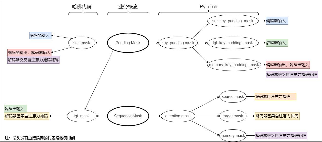
The figure contains Chinese labels, but its central split is readable:
attention mask:
    relation between query positions and key positions
    examples: causal triangle, memory restriction, block-diagonal packing

key padding mask:
    which key columns correspond to real tokens in each batch row
For torch.nn.Transformer, the common public objects are:
| API object | Logical shape | Applies to |
|---|---|---|
src_mask | [S,S] or head/batch-expanded form | encoder source-position relation |
tgt_mask | [T,T] or expanded form | decoder target relation, normally causal |
memory_mask | [T,S] or expanded form | decoder-query to encoder-memory relation |
src_key_padding_mask | [B,S] | source key columns |
tgt_key_padding_mask | [B,T] | target key columns |
memory_key_padding_mask | [B,S] | encoder-memory key columns during cross-attention |
These names are API contracts, not six independent mathematical ideas. At the
score boundary they become a relation broadcastable to [B,H,Q,K]. A wrapper
may combine them; a fused kernel may receive only cumulative lengths and an
is_causal flag. Parity means all encodings exclude the same edges.
Teacher-forced training: future rows exist but remain illegal
During decoder training, the target batch commonly contains the whole shifted target sequence:
decoder input:  <bos> y_0 y_1 ... y_(T-2)
labels:          y_0  y_1 y_2 ... y_(T-1)
All input rows can be processed in parallel because row i is prevented from
reading rows j > i. The target causal mask and the label shift solve
different problems:
causal visibility:
    prevents hidden-state leakage inside the model

label shift:
    chooses which next token each output row predicts

loss padding mask:
    chooses which output rows contribute to the objective
Applying only two of the three can produce plausible loss curves with the wrong task. In particular, masking PAD keys does not automatically remove PAD query rows from cross-entropy.
The handwritten mask article followed the same objects through the encoder and both decoder attention calls:
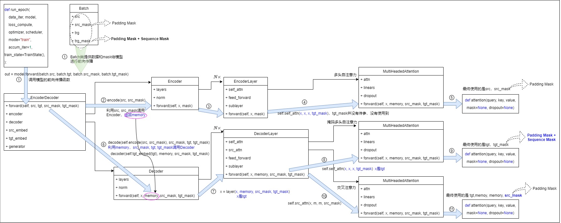
The operational call graph is:
memory = encoder(src_states, src_visibility)

target_states = decoder_self_attention(
    target_states,
    target_states,
    target_states,
    target_visibility,       # causal AND target-key-real
)

target_states = cross_attention(
    target_states,
    memory,
    memory,
    source_key_visibility,   # source columns, no target triangle
)
When S == T, swapping the last two masks may preserve every tensor shape.
The semantics still fail. This is why call-site tests need unequal source and
target lengths.
Prefill, one-token decode, and static cache buffers
At inference prefill, a decoder-only model processes a prompt block with a causal relation over prompt rows. After prefill, ordinary one-token decode may have:
Q = 1
K = past_length + 1
If the K/V tensor contains exactly the contiguous legal prefix, every supplied key is legal for the current query and the kernel can omit an explicit dense triangle. That optimization is a consequence of cache extent and absolute positions, not a change in causal semantics.
Explicit validity becomes necessary again when physical extent exceeds legal state:
static cache:
    allocated slots beyond current length must stay invisible

left-padded batch:
    physical columns before the real prefix may be PAD

chunked decode:
    several new queries need a local causal relation inside the chunk

speculative branch:
    candidate rows may have branch-specific ancestry

sliding window:
    old but physically retained keys may be outside the legal window
The backend may encode these cases through lengths, cache positions, block
tables, or a custom mask. The model-level audit remains the predicate
legal(query_position,key_position).
Packing is a joint attention, position, and loss contract
Padding a batch to its longest sequence can waste most token slots when length distributions are broad.
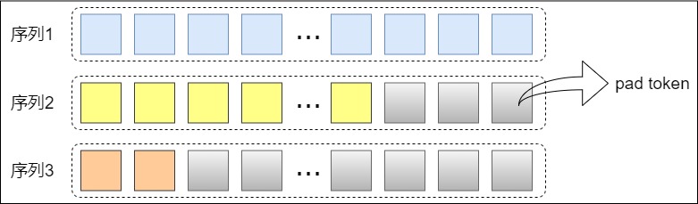
Packing removes that waste by concatenating independent examples into fewer physical rows:
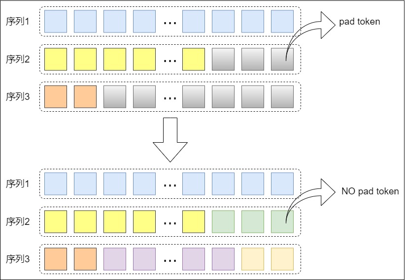
But concatenation alone silently changes the training problem. A correct packed representation needs at least:
token IDs:
    the physical packed row

segment or cumulative-length metadata:
    which tokens belong to one logical example

position IDs:
    whether positions reset per example or follow another documented policy

attention visibility:
    block-diagonal causal edges, no cross-example reads

loss boundaries:
    labels must not predict the first token of the next packed document from
    the final token of the previous document unless that transition is intended
For example lengths [3,4,5,4], cumulative boundaries are:
cu_seqlens = [0,3,7,12,16]
A variable-length attention kernel can consume those boundaries and run the
four causal examples without constructing a dense 16 x 16 block mask. The
dense block-diagonal matrix and cu_seqlens are semantically equivalent only
if query/key ordering and position policy agree.
The LongAlign figure retained by A11 shows that packing also has a scheduling dimension: filling token capacity does not guarantee balanced per-rank work or equal example weighting.
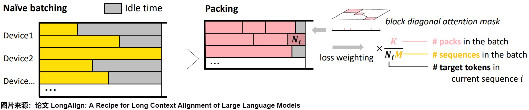
Three concerns should be measured separately:
padding efficiency:
    fraction of physical token slots carrying real tokens

compute balance:
    whether workers receive comparable sequence work

optimization weighting:
    whether long examples dominate because loss is averaged per token rather
    than per logical example
The source packing survey compares combinations of sorting, padding, fixed length packing, position IDs, and document isolation:
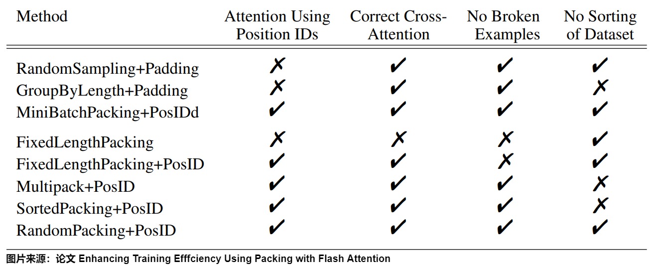
The figure is a source-reported design comparison, not a universal ranking. The correct choice depends on whether the workload permits truncation, whether the kernel accepts variable lengths, how distributed batches are balanced, and how the loss weights examples. The non-negotiable correctness rule is simpler:
tokens from independent examples must not exchange attention or labels unless
the dataset explicitly defines that relation.
Packing conformance test
A minimal test compares packed and unpacked execution with dropout disabled:
def assert_packed_equivalence(model, examples, pack):
    separate = [model(x, causal=True) for x in examples]

    packed_ids, segment_ids, positions = pack(examples)
    packed_out = model(
        packed_ids,
        segment_ids=segment_ids,
        position_ids=positions,
    )

    cursor = 0
    for expected, example in zip(separate, examples):
        length = example.shape[-1]
        actual = packed_out[:, cursor:cursor + length]
        torch.testing.assert_close(actual, expected, rtol=1e-4, atol=1e-5)
        cursor += length
This catches cross-example leakage, position-reset mistakes, and wrong cumulative boundaries. A separate label test must confirm that loss transitions also stop at document boundaries.
0x07 Softmax over key positions
The visible text covers the softmax axis, why subtracting the row maximum is exact and what it does and does not protect against, how softmax turns score differences into probability ratios, and how adding legal keys dilutes a fixed score gap. Two symbols come from the folded blocks: is the set of legal keys in one query row, and is that row’s log-sum-exp. The folds hold the theory of softmax (log-sum-exp, Jacobian, temperature, entropy), alternative normalizers, exceptional rows, and the online form used by fused kernels.
After bias and mask:
p_attn = scores.softmax(dim=-1)
The dim=-1 is the key/value axis:
p_attn: [B, h, q_len, k_len]
For each batch item, head, and query row:
sum_j p_attn[b, head, i, j] = 1
That means each query row forms a distribution over visible key/value rows.
Wrong-axis softmax keeps the same rank but changes the operation:
scores.softmax(dim=-2) # wrong for normal attention
That would normalize over query rows. Instead of each query choosing keys, each key would distribute mass across queries. The tensor shape survives; the row ownership does not.
How this was checked The exact domain assumed here (a non-empty set of legal keys with finite scores) and what is left to the mask and dropout steps; open it for the formal setting of this section. (about 190 words, 1 code listing, 4 equations)
Loop 5 contract: normalize one finite legal row
Loop 4 froze the support relation. For one fixed [batch, head, query] row,
let
be the legal key indices and let s_j denote the finite scaled score plus any
finite position bias for j in J. Loop 5 owns the map
It does not choose J, move a key into or out of the support, define a
dropout realization, or choose an IO-aware kernel schedule. Those boundaries
matter because four objects that are often called “the softmax row” are not
interchangeable:
| Object | Contract | Owner after this loop |
|---|---|---|
semantic support J | which key positions may receive mass | frozen by Loop 4 |
legal logits s_J | finite compatibility values on that support | Loops 3-4 |
pre-dropout distribution p | nonnegative, unit-sum routing mass over J | Loop 5 |
| post-dropout weights | stochastic rescaled coefficients; one realization need not sum to one | Loop 6 |
The strict reference domain is therefore:
support is non-empty;
every legal score is finite;
masked entries are absent from the reduction;
normalization is over the key axis;
probabilities are inspected before attention dropout.
NaN, legal +inf, legal -inf, and empty support are explicit policy
boundaries later in this section. They are not silently repaired by changing
the formula.
Derivation Softmax as the gradient of log-sum-exp, which explains why a constant shift changes nothing, and as a score-plus-entropy maximization; open it for the theory behind the visible identities. (about 290 words, 1 code listing, 16 equations)
One log-partition function generates the entire row geometry
Define the log-partition function on the legal support:
Differentiate it with respect to one legal score:
Thus softmax is not an unrelated activation placed after the score function:
This one identity will generate the translation invariance, probability ratios, Jacobian, entropy relation, and temperature derivatives below. It also fixes the difference between a probability and its normalizer:
A(s):       one scalar log-normalizer for the row
p_i:        one derivative of that scalar with respect to score i
sum_i p_i:  one, because all legal terms share the same denominator
Adding a common constant c gives
so its gradient is unchanged:
The logits are consequently identifiable only up to a common row offset. Two implementations can use different representatives of the same row and still produce exactly the same real-arithmetic probabilities.
Softmax is entropy-regularized competition
Softmax also solves a constrained optimization problem:
where
Introduce a Lagrange multiplier for sum_j p_j = 1. For an interior optimum,
Therefore p_j is proportional to exp(s_j), and normalization recovers
softmax. The score term rewards concentrating on large logits; Shannon entropy
rewards spreading mass. Temperature changes the strength of that competition.
Removing or replacing softmax is therefore a model change, not merely deleting
one expensive function call.
Stable softmax and why subtracting the row maximum is exact
The mathematical softmax is invariant to adding the same constant to every logit in one row:
Choose c = max(scores[row]). The largest shifted logit is zero, so no shifted
exponential is greater than one:
row_max = masked_scores.max(dim=-1, keepdim=True).values
shifted = masked_scores - row_max
probabilities = shifted.exp()
probabilities = probabilities / probabilities.sum(dim=-1, keepdim=True)
This is not an approximation to softmax. It is the same distribution evaluated with a numerically safer representative of the logit row. Blanchard, Higham, and Higham analyze this distinction directly: formulas that are equivalent in real arithmetic can have different overflow, underflow, and rounding behavior in finite precision.
The stable row can be written as a compact state:
Then:
At least one shifted score is zero. If n = |J|, every shifted exponential
lies in (0,1], and therefore:
These bounds explain exactly what subtract-max repairs. It prevents positive exponential overflow for finite legal logits and keeps the denominator in a known range. It does not guarantee that every small term remains representable. A large negative gap can still underflow:
ideal real arithmetic:
    exp(s_j - m) is positive for every finite legal score

finite precision:
    a sufficiently negative s_j - m may round exp(...) to zero
That zero is numerical truncation, not semantic sparsity. It can be harmless for a negligible forward contribution while still erasing the corresponding small gradient. The required accumulation dtype and error tolerance are therefore part of the implementation contract.
For an explicit eager path, keep the reduction dtype visible:
def stable_softmax_finite_row(scores, visible, work_dtype=torch.float32):
    legal = scores[visible]
    if legal.numel() == 0:
        raise ValueError("softmax support is empty")
    if not torch.isfinite(legal).all():
        raise ValueError("legal softmax scores must be finite")

    work = legal.to(work_dtype)
    row_max = work.max()
    numerators = torch.exp(work - row_max)
    denominator = numerators.sum()

    probabilities = torch.zeros_like(scores, dtype=work_dtype)
    probabilities[visible] = numerators / denominator
    logsumexp = row_max + denominator.log()
    return probabilities, logsumexp
PyTorch’s functional softmax exposes a dtype argument that casts before the
operation, specifically allowing callers to choose a safer computation type.
torch.logsumexp exposes the stabilized log-normalizer directly. Neither API
removes the need to validate the axis, legal support, or exceptional inputs.
A deterministic NumPy reference on shifted logits [0,-10,-20,-40] makes the
precision boundary concrete:
| Work dtype | Stable exponential numerators, approximately | Resulting observation |
|---|---|---|
| float16 | [1, 4.54e-5, 0, 0] | gaps 20 and 40 underflow to exact stored zeros; adding 4.54e-5 to 1 also rounds the denominator to 1 |
| float32 | [1, 4.54e-5, 2.06e-9, 4.25e-18] | all four terms remain represented in this fixture |
| float64 | [1, 4.54e-5, 2.06e-9, 4.25e-18] | reference retains the same terms with a more accurate sum |
These are fixture observations, not universal hardware thresholds. Subnormal handling, reduction precision, flush-to-zero behavior, and fused-kernel policy can differ. The invariant is the diagnostic method: record the work dtype, test adversarial score gaps, and compare against a higher-precision reference.
Fused kernels perform an equivalent running-max/running-sum reduction in tiles. They do not need to materialize the full score matrix to preserve exact softmax semantics. M4.3 owns the online-state merge proof, pass/access accounting, value-numerator recurrence, and IO reason for fusing score, mask, normalization, and value accumulation.
Probability ratios reveal what softmax preserves
For two legal keys j and r in one query row:
Softmax discards a common row offset but preserves every pairwise logit difference as a probability ratio. This gives three useful consequences:
adding the same constant to a row changes nothing;
multiplying logits changes sharpness because it scales every difference;
masking a key with -infinity makes its ratio to a legal key zero.
The A10 visual below shows both the row-wise probability calculation and the query-by-key matrix whose final axis is normalized:
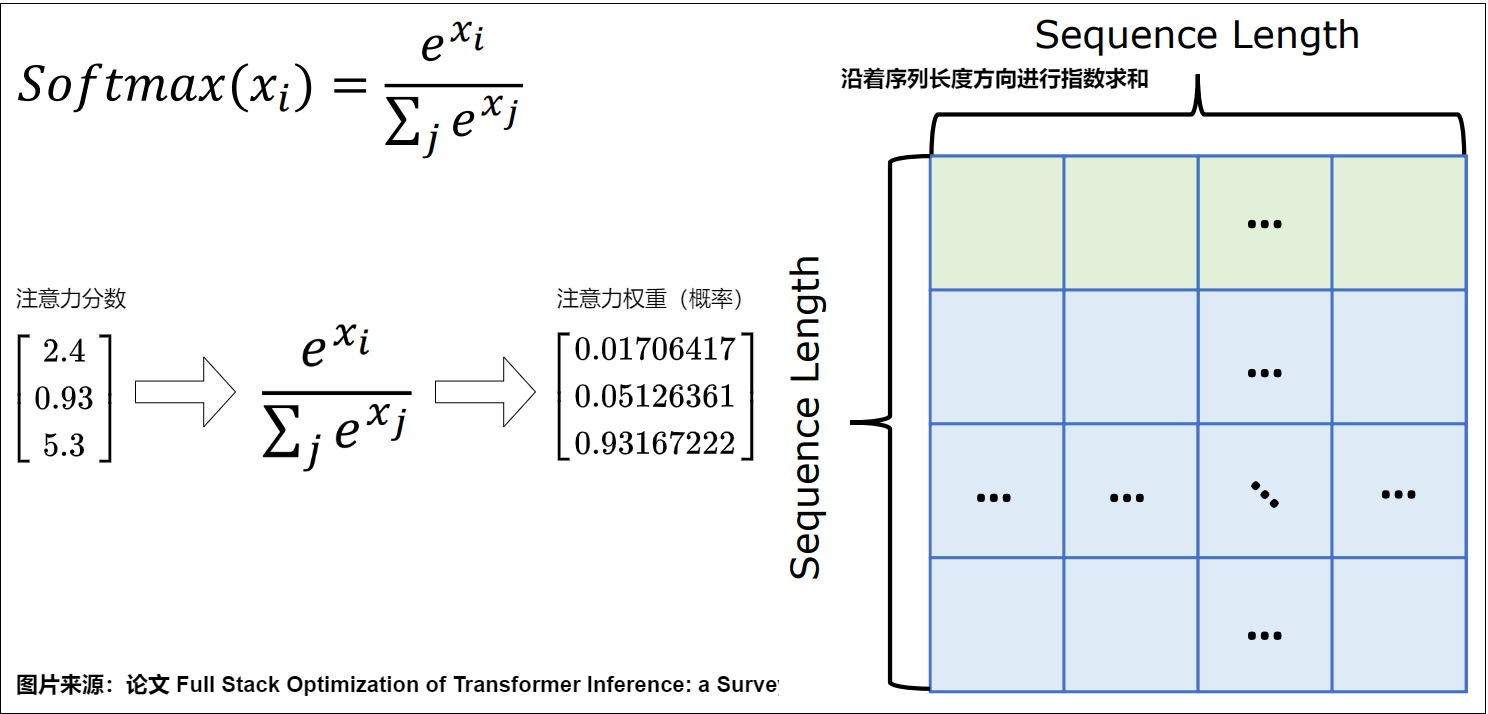
The numerical labels are illustrative. The semantic point is that softmax is
applied independently to every [batch,head,query] row, never once over the
whole matrix.
The ratio identity also proves three order properties for finite legal scores:
Softmax changes magnitudes but not score ordering. It is also dense on a finite legal support:
Exact zeros in the ideal distribution come from support exclusion or a different normalizer, not from an ordinary finite softmax score. Finite precision can round a tiny positive value to zero, but that numerical event must not be mistaken for a learned sparse-support decision.
Derivation The softmax Jacobian and how it couples every key in a row, saturation from a large gap (with ties and single-key rows), and how temperature changes entropy; open it before the backward pass or entropy diagnostics. (about 660 words, 1 code listing, 30 equations)
The softmax Jacobian and gradient coupling
For probability vector p = softmax(s), the derivative is:
In matrix form:
The off-diagonal terms are not zero. Raising one logit changes all
probabilities because the row must continue to sum to one. Given upstream
gradient g_p, the efficient vector-Jacobian product is:
This form appears later in the full backward trace. It also explains why inspecting each attention edge independently is incomplete: legal edges in the same row compete through normalization.
The same matrix is the Hessian of the log-partition function:
For any vector z over the legal keys,
So the Jacobian is symmetric positive semidefinite. Its constant direction is null:
This is the differential form of row-offset invariance. If all n legal
probabilities are positive, the Jacobian has rank n-1: softmax maps an
n-coordinate logit row onto the interior of an (n-1)-dimensional
probability simplex. No gradient can identify or update a common score offset
through this operation alone.
The covariance reading is also an implementation test. A computed Jacobian
should be symmetric, have row and column sums near zero, and have no materially
negative eigenvalue beyond the declared numerical tolerance. Those checks are
stronger than testing only sum(p) = 1.
Saturation from a large logit gap
For two logits [0, delta]:
As delta grows, p_2 approaches one and the derivative approaches zero.
Scaling by sqrt(d_k) is therefore connected directly to optimization: it
reduces dimension-driven logit gaps before softmax. It does not guarantee high
entropy after training; the model can still learn sharp distributions.
Two boundary cases sharpen that statement:
one legal key:
    p = [1] and J = [0] for every finite score;
    this is structural certainty, not a numerical failure

tied largest scores:
    lowering temperature does not choose one tied key;
    the limiting mass is shared uniformly across the maximal set
For example, softmax(alpha * [3,3,1]) approaches [0.5,0.5,0] as
alpha -> infinity, not a one-hot vector. An implementation oracle must
include ties and singleton support instead of testing only a unique maximum.
Entropy is descriptive, not an objective by default
The entropy of one attention row is:
Uniform attention over n legal keys has entropy log(n); a one-hot limit has
entropy zero. Temperature controls this distribution:
Increasing tau flattens the row; decreasing it sharpens the row. But low
entropy is not automatically “better focus,” and high entropy is not
automatically “confusion.” A head may need a broad average, a special-token
sink, a local copy, or a sparse retrieval depending on layer and task. Unless
the training loss contains an explicit entropy term, entropy is a diagnostic
of the learned routing distribution rather than a direct target.
The log-partition identity gives a more precise temperature path. Let
alpha = 1 / tau >= 0 and
Differentiate one probability:
Large-score keys gain mass and below-mean keys lose mass. The expected score obeys
Using
we obtain
For nonnegative inverse temperature, sharpening cannot increase entropy in
exact arithmetic. Equality holds when the legal scores are all equal or at
alpha = 0. The endpoints are:
and, as alpha -> infinity, uniform mass over the set of maximal scores. This
derivation is row-local. It does not establish that changing temperature
improves a trained model, preserves calibration, or generalizes across context
lengths.
Legal support size can dilute attention without changing old logits
A10 raised a separate length-generalization problem: even if the logits for existing keys do not change, adding more legal keys changes the softmax denominator.
Suppose one relevant key has logit a and n distractors all have logit b,
with gap Delta = a-b. The relevant probability is:
For fixed Delta, increasing n lowers the relevant key’s probability. To
hold probability at target p^*, the required gap is:
This is a clean derivation of mass dilution. It does not say every long context becomes uniform: real distractor logits differ, position mechanisms change scores, and trained heads can increase the relevant gap. It says that softmax competition depends on the number and scores of all legal keys, not only the best pair.
A10 discussed this issue using an earlier title of the linked preprint. The current v3 is titled Softmax is not Enough (for Sharp Size Generalisation). Its externally verified claim is narrower than “softmax always becomes uniform”: for sharp tasks such as maximum-key selection, a fixed learned softmax circuit can disperse as valid problem size grows, and the paper studies adaptive temperature as an ad-hoc mitigation. The algebra above is a toy equal-distractor case that makes one denominator pressure visible; it is not a reproduction of every theorem or experiment in that paper.
The same argument applies when m relevant keys share logit a:
This form distinguishes adding useful evidence from adding distractors.
For a fixed gap Delta = 4, the one-relevant-key fixture gives:
Equal-logit distractors n | Relevant-key probability |
|---|---|
| 1 | 0.9820 |
| 4 | 0.9317 |
| 16 | 0.7734 |
| 64 | 0.4604 |
If the target relevant probability is 0.9, the required gaps for those same
support sizes are approximately 2.197, 3.584, 4.970, and 6.356.
Quadrupling distractor count adds log(4) to the required gap. The executable
oracle derives these values from the formulas rather than storing them as
unexplained examples.
Worked detail Why rescaling logits with context length changes the model rather than extending it exactly, and row diagnostics that say more than one mean entropy; open it when studying long-context behaviour. (about 190 words, 2 code listings, 2 equations)
Length-dependent temperature is a model change
A10 discusses scaling logits as context length changes, schematically using a
factor related to log(n)/log(m) for inference length n and training length
m. The motivation follows from the gap equation: sharper logits can offset a
larger legal support.
Write a general multiplier c(n):
Increasing c(n) lowers the effective temperature and amplifies every score
difference. This may preserve concentration in some distributions, but it is
not an algebraically exact context extension. It changes attention weights,
can over-sharpen already decisive rows, interacts with position geometry, and
may alter behavior on heads that intentionally average broadly.
The claim should therefore be scoped:
source-local motivation:
    longer legal support can increase entropy or dilute fixed score gaps

rewrite interpretation:
    length-dependent logit scaling is one possible compensation

not guaranteed:
    one scaling law preserves quality or entropy for every head and input
M3.5 owns the full context-extension comparison, because score scaling must be evaluated beside RoPE frequencies, interpolation, fine-tuning, retrieval tests, and serving constraints.
Better diagnostics than one mean entropy number
For one attention row, useful diagnostics include:
entropy H(p):
    overall uncertainty, depends on support size

normalized entropy H(p)/log(n_legal):
    concentration relative to the maximum for that legal support

effective support exp(H(p)):
    number of equally weighted keys with the same entropy

top-k mass:
    how much probability lies in the largest k entries

maximum probability and logit gap:
    sharpest edge and separation from competitors

mass on designated evidence spans:
    task-conditioned retrieval diagnostic, when labels exist
These measurements should be stratified by layer, head, query type, and context length. Averaging all rows can hide a mixture of one-hot copy heads and broad aggregation heads.
Alternatives and history Why vocabulary methods such as hierarchical softmax do not apply here, and how sigmoid gates, sparsemax and entmax change the routing; open it when considering a different normalizer. (about 340 words, 2 code listings, 2 equations)
Attention softmax is not vocabulary softmax
A10 also surveys log-softmax, hierarchical softmax, and adaptive softmax. Those methods primarily address output distributions over a large vocabulary. They are not direct replacements for attention normalization over key positions.
vocabulary softmax axis:
    candidate token IDs, often tens or hundreds of thousands

attention softmax axis:
    legal key/value rows for one query
Log-softmax is valuable when a downstream loss consumes log probabilities, but
attention needs probabilities or an equivalent normalized value accumulator
for P@V. Hierarchical/adaptive vocabulary methods exploit token-frequency and
class structure; key positions in one attention row do not follow that fixed
vocabulary tree.
This is a deliberate non-import from the handwritten source: the broader softmax background remains useful in A10, while M3.1 retains only methods whose axis and contract match attention.
Alternative row normalizers change the routing geometry
The design space is broader than ordinary softmax, but each alternative gives up at least one part of the contract just derived:
| Mapping | Row coupling | Exact zeros from finite legal scores? | Geometry and runtime consequence |
|---|---|---|---|
| softmax | one exponential denominator | no | interior of simplex; smooth dense competition |
| independent sigmoid gates | no shared denominator | no | total row mass is not fixed; keys do not compete globally |
| sparsemax | Euclidean projection onto simplex | yes | piecewise-linear sparse support and a different Jacobian |
alpha-entmax | generalized entropy regularization | yes for alpha > 1 | interpolates from dense softmax toward sparse mappings |
| unnormalized or kernel attention | method-specific | method-specific | changes normalization, associativity, and often the runtime graph |
Sparsemax is defined as a simplex projection:
Unlike finite-logit softmax, the projection can land on the simplex boundary
and assign exact zero mass. Martins and Astudillo derived its Jacobian and
applied it to neural attention. Peters, Niculae, and Martins later introduced
alpha-entmax sequence models, where softmax and sparsemax are members of a
larger family and alpha > 1 can produce sparse alignments.
These alternatives are not drop-in numerical fixes for an unstable softmax:
switching normalizer changes forward probabilities;
switching normalizer changes gradients and learned optima;
exact sparsity does not automatically produce kernel speedup;
checkpoint weights trained with one map need not preserve behavior under another.
Loop 5 records this comparison so that “tiny floating-point probability” is not confused with “model-defined zero support.” M3.1 Loop 9 owns the full alternative-interaction comparison, including kernel/linear attention and the M4 runtime boundary.
Edge cases and failure behaviour What the normalizer should do with empty rows and with infinite or NaN scores, and why repairing NaN after softmax hides the cause; open it when a row returns NaN. (about 230 words, 1 code listing)
Exceptional rows need policy before arithmetic
Subtract-max softmax has a finite-input contract. Applying it blindly to extended or undefined values produces ambiguous or invalid operations:
| Legal row presented to the normalizer | What the formula asks for | Strict M3.1 policy |
|---|---|---|
| non-empty, all finite | ordinary stable softmax | compute |
| empty support | denominator is an empty sum | reject a consumed query or route an explicit unused-row policy |
all entries -inf | -inf - (-inf) | do not call ordinary softmax; this is empty effective support |
one legal +inf | inf - inf after subtract-max | reject or invoke a separately specified extended-real policy |
multiple legal +inf | limit depends on how infinities are approached | reject or explicitly define mass sharing |
any legal NaN | comparisons and exponentials are contaminated | reject and diagnose the upstream producer |
finite legal row plus masked -inf storage | masked entries are outside J | compute over legal entries only |
A convenient extended-real convention could assign all mass to one +inf, or
split mass uniformly across several +inf entries. That convention is not the
ordinary real-valued softmax formula, and different frameworks need not infer
it. The strict oracle used here rejects non-finite legal logits and allows
-inf only as a physical encoding of an already-excluded entry.
Do not repair an undefined row after the fact:
# Too late: the reduction has already lost the semantic distinction.
probabilities = torch.nan_to_num(torch.softmax(scores, dim=-1))
This can turn empty support, an upstream NaN, and a legal +inf into the same
zero-filled symptom. Validate support and finiteness before normalization so
the failure retains its cause.
Masking as a probability limit
For a blocked key, add mask value -C and let C grow:
This is the mathematical reason for an additive negative-infinity mask. A
large finite constant approximates the limit, but the result depends on dtype
range and implementation. In float16, a literal -1e9 cannot be represented
as a finite value and becomes -inf; other constants may remain finite and
leave tiny nonzero mass.
The ideal mask also removes score gradients through blocked entries because their probability is zero. That statement is local to the attention-score path. The underlying token row can still receive gradients through query-side work, residual branches, embeddings, or another attention call.
Derivation Proof that naive, max-subtracted and tile-by-tile (online) softmax share one denominator, a reference online normalizer, and the row [1000, 999, 998] worked through; open it before reading about fused kernels. (about 370 words, 2 code listings, 12 equations, 1 figure)
Naive, safe, and online normalization are the same row contract
A10 retained a two-pass naive softmax algorithm: first accumulate the denominator, then divide each exponential.
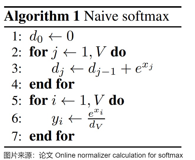
The direct algorithm is mathematically clear but numerically unsafe if logits are large. For a finite row, define its native denominator
Subtracting the final maximum m gives
The common e^m cancels from every probability:
Safe softmax therefore changes coordinates, not the ideal row distribution.
Online softmax changes when those same coordinates are discovered. Suppose a
prefix has state (m_old, ell_old) and an incoming tile has maximum m_tile.
Choose one common reference:
Every old and incoming exponential must be expressed under that reference:
By induction, after the final tile:
Native, safe, scalar-online, and block-online normalization thus share one denominator in exact arithmetic. They are not necessarily bitwise identical in finite precision because reduction and merge order change rounding.
The smallest auditable online normalizer keeps an explicit validity branch so
the empty-state identity never evaluates -inf - (-inf):
def online_normalizer(finite_scores):
    valid = False
    running_max = -float("inf")
    running_sum = 0.0

    for score in finite_scores:
        if not math.isfinite(score):
            raise ValueError("legal score must be finite")
        if not valid:
            running_max = score
            running_sum = 1.0
            valid = True
            continue

        new_max = max(running_max, score)
        running_sum = (
            running_sum * math.exp(running_max - new_max)
            + math.exp(score - new_max)
        )
        running_max = new_max

    if not valid:
        raise ValueError("softmax support is empty")
    return running_max, running_sum
For the adversarial row [1000, 999, 998], direct exponentiation overflows in
ordinary floating-point arithmetic. Subtract-max and online normalization both
reduce it to the finite gaps [0,-1,-2] and produce approximately:
[0.66524096, 0.24472847, 0.09003057]
The A10 image is sourced from Milakov and Gimelshein’s online-normalizer paper. It captures the naive two-scan denominator, but not the safe maximum pass or the online recurrence. The existing M4.3 visual below supplies that missing algorithm comparison:

M3.1 owns the distribution identity, strict finite-row domain, and parity oracle. M4.3 owns scan/access counts, merge trees, online value numerators, FlashAttention scheduling, HBM traffic, and backward reconstruction. Carrying the same recurrence here is a semantic handoff, not a second kernel chapter.
How this was checked The softmax properties the article's test code checks (shift, gradient, curvature, temperature, support size, precision, exceptional inputs); open it when writing your own softmax tests. (about 40 words, 1 code listing)
Loop 5 executable gate
The publication oracle exercises properties that a shape-only example misses:
translation:
    softmax(s + c) == softmax(s)

partition gradient:
    finite_difference(grad(logsumexp)) == softmax(s)

curvature:
    J == diag(p) - p p^T
    J is symmetric positive semidefinite
    J @ ones == 0

temperature:
    entropy is non-increasing with nonnegative inverse temperature
    tied maxima share limiting mass

support:
    singleton -> p=[1], J=[0]
    empty support -> explicit error

finite precision:
    native overflow is observable
    subtract-max avoids positive overflow
    low precision may underflow tiny legal probabilities to zero

exceptional input:
    legal NaN, +inf, and -inf are rejected before reduction
The oracle also reconciles scalar-online and block-online states against the same stable reference. It does not benchmark a GPU kernel; that experiment belongs to M4.3.
0x08 Dropout on attention probabilities
The Harvard code applies dropout to p_attn:
if dropout is not None:
    p_attn = dropout(p_attn)
So the local order is:
scores
  -> mask
    -> softmax
      -> dropout on p_attn
        -> p_attn @ value
This is not dropout on the value tensor and not dropout on raw scores.
Modern functional APIs can have their own sharp edges. PyTorch’s scaled_dot_product_attention applies dropout according to the dropout_p argument, so callers must pass 0.0 during evaluation if they use the functional form directly.
The conceptual point for M3.1 is simple:
attention dropout changes which probability links are active during training.
it does not change which keys are legal.
Legality is still the mask.
How this was checked The objects of one dropout draw (keep mask, rescaling factor, consumed weights) with their shapes, and where the placement on probabilities comes from; open it for the setup used by the derivations below. (about 320 words, 4 equations)
Loop 6 contract: one realized stochastic local operation
Loop 5 ended with a deterministic pre-dropout probability tensor. Loop 6 adds one random object, uses it to mix values, and then differentiates that exact realization. For one batch/head/query row, write:
The consumed routing weights and head output are:
The distinction among these objects is part of the training contract:
| Object | Shape | Deterministic after inputs? | Semantic role |
|---|---|---|---|
| legal support | [B,H,Q,K] predicate | yes | which query-key edges may exist |
P | [B,H,Q,K] | yes | normalized pre-dropout routing distribution |
M | [B,H,Q,K] boolean | no during training | sampled kept/dropped edges |
Z=M/(1-rho) | [B,H,Q,K] | no during training | inverted-dropout multiplier |
Pdrop=P*Z | [B,H,Q,K] | no during training | weights actually consumed by V |
V | [B,H,K,Dv] | yes after the forward inputs are fixed | payload rows |
O=Pdrop@V | [B,H,Q,Dv] | no during training | contextualized per-head output |
dO | [B,H,Q,Dv] | supplied by later computation | upstream backward signal |
This loop owns the dense semantic equations, their tensor shapes, one fixed-RNG gradient trace, and the state required to reproduce that trace. It does not own how a tiled kernel visits query/key blocks, where those blocks live, or which gradient tile has exclusive hardware ownership. Those schedules remain in M4.3.
Historically, general dropout randomly removes units or connections during
training to reduce co-adaptation. Srivastava et al.
provide that general contract. The Annotated
Transformer makes the
attention-specific placement explicit in code: normalize scores, drop entries
of p_attn, then multiply by value. That placement is a model choice, not an
algebraic consequence of softmax.
Inverted attention dropout is unbiased only in expectation
Let pre-dropout probability be p_ij. With dropout probability rho, draw
independent mask m_ij ~ Bernoulli(1-rho) and use inverted scaling:
Then:
The expected value mix is unchanged:
But one realized row generally does not sum to one:
Derivation Variances of the dropped probabilities, the row sum and the output, the chance that a whole row drops, and a Monte Carlo check of these formulas; open it to quantify dropout noise. (about 250 words, 1 code listing, 12 equations)
Its element-wise variance is:
The row sum is a random variable:
Assuming independent Bernoulli draws across legal edges:
This variance depends on concentration. A diffuse row has small
sum_j p_ij^2; a nearly one-hot row inherits almost the full
rho/(1-rho) variance of one Bernoulli multiplier. If a row has n_i legal
keys, its probability of losing every legal route is:
That event is legal under ordinary element-wise attention dropout. It produces a zero head-output row for this attention call; it is not the same condition as an all-masked softmax row, which Loop 4 rejects before normalization.
The output is also an unbiased random estimator:
Its covariance under independent edge draws is:
The covariance is value-dependent. Attention dropout therefore injects noise in the payload directions selected by the routing distribution; it is not just noise in a scalar probability diagnostic.
The Loop 6 oracle checks these equations with 200,000 fixed-seed draws for:
P = [0.1, 0.2, 0.3, 0.4]
rho = 0.2

analytic E[row sum]       = 1.000000
empirical E[row sum]      = 1.000564
analytic Var(row sum)     = 0.075000
empirical Var(row sum)    = 0.075137

analytic E[output]        = [0.800000, 0.975000]
empirical E[output]       = [0.798995, 0.975084]
Pr(all four routes drop)  = 0.001600
These are deterministic fixture results, not a benchmark or a claim that independence is the only useful dropout structure.
This resolves an apparent contradiction in debugging:
before dropout:
    each legal probability row sums to one

after dropout during training:
    individual rows need not sum to one

in expectation:
    the original probability and value mixture are preserved
Frameworks also differ in which object they expose as “attention weights.”
Some return pre-dropout probabilities for interpretation; the Harvard helper
stores self.attn before or around the dropout path depending on the wrapper;
fused kernels may not return the matrix at all. Tests must name the object they
expect instead of asserting row sums on an undocumented tensor.
Derivation Why one realized output after dropout is a rescaled rather than a convex combination of values, with numbers from one fixed draw; open it if outputs after dropout look shifted. (about 120 words, 4 equations)
One realization is not a convex combination
Before dropout, P_i V lies in the convex hull of the visible values. After
dropout, every coefficient remains nonnegative, but the coefficient sum is
R_i, not necessarily one. A realized output is therefore a nonnegative,
rescaled combination, not generally a convex combination.
This changes a useful translation identity. Add one constant vector c to
every visible value row. Before dropout:
For one post-dropout realization:
Only in expectation does the shift return to c. In the fixed oracle trace,
the two realized row sums are 1.004632 and 0.990504; adding
c=[2,-1.5] consequently adds [2.009265,-1.506949] and
[1.981008,-1.485756], respectively.
Alternatives and history Other dropout placements (renormalizing survivors, dropping keys before softmax, DropAttention, DropKey, DropHead) and why each is a different estimator, with a worked example; open it before changing the dropout scheme. (about 300 words)
Alternative dropout placements are different estimators
“Apply dropout to attention” does not identify one operation. The dropped object, placement relative to softmax, sharing pattern, schedule, and fallback policy all change the training distribution.
| Design | Random object | Row normalized in one realization? | Key consequence | Owner here |
|---|---|---|---|---|
| standard attention-weight dropout | independent entries of post-softmax P | no | Pdrop@V is unbiased after inverted scaling | derived fully |
| drop then renormalize survivors | post-softmax entries, followed by division by surviving mass | yes unless every route drops | changes expectation and needs an all-drop fallback | comparison only |
| pre-softmax key/edge deletion | support or logits before normalization | yes if support stays nonempty | recomputes competition over surviving keys | comparison only |
| DropAttention | elements, columns, or contiguous regions of the attention matrix | method-dependent | introduces structured correlation across dropped routes | paper boundary |
| DropHead | one multiplier for an entire head | no at head-combination boundary | regularizes head co-adaptation rather than individual routes | M3.2 boundary |
| value/output/residual dropout | value features or later sublayer output | not a routing-row question | perturbs payload channels or residual writes | M3.7 boundary |
DropAttention studies element-, column-, and contiguous-region structures over attention weights. DropKey moves stochastic deletion before attention normalization for vision Transformers. Scheduled DropHead drops whole heads and changes the rate across training. Their reported quality results belong to their tasks and settings; the reusable point here is that they randomize different semantic objects.
Renormalization is especially easy to mislabel as an implementation detail.
Enumerating every keep mask for P=[0.1,0.2,0.7] and rho=0.5 gives:
| Rule | Expected realized weights |
|---|---|
| inverted dropout, no renormalization | [0.1000, 0.2000, 0.7000] |
| renormalize survivors, all-drop becomes zero | [0.1948, 0.2611, 0.4191] |
renormalize survivors, all-drop falls back to original P | [0.2073, 0.2861, 0.5066] |
Both renormalized variants bias the expected routing weights in this unequal row. Preserving row sum one and preserving the original expectation are not the same contract.
Implementation and runtime contracts The random-number state backward needs to replay the same mask, why evaluation must pass dropout_p=0.0 to PyTorch's functional call, and how precision and backend affect the score path; open it when training runs are not reproducible. (about 350 words, 3 code listings, 1 figure)
RNG state is part of the training input
For gradient derivation, M is held fixed. Backward differentiates the sampled
program that ran in forward; it does not differentiate the Bernoulli sampling
decision and must not draw a fresh mask. Reproducible execution therefore needs
more than a nominal dropout probability:
global/model seed
device-specific generator identity
generator seed and counter/offset before the operation
logical batch, head, query, and key coordinates
draw-to-coordinate mapping
training/evaluation mode and dropout probability
A saved dense mask is sufficient but can be quadratic. A fused implementation
may instead save compact generator state and replay each logical draw. Saving a
seed alone is insufficient if a changed tile order, vector width, or counter
advance maps that seed to different (batch,head,query,key) coordinates.

The visual is reused from M4.3 because the semantic objects are identical. M3.1 owns why replay is required. M4.3 owns how tiled forward/backward regenerate those objects without materializing the global probability or mask matrices.
PyTorch’s functional.dropout
takes an explicit training flag. Its functional
scaled_dot_product_attention
has a sharper contract: it applies dropout whenever dropout_p > 0, so a module
wrapper must pass 0.0 explicitly during evaluation.
Precision, dtype, and backend are implementation contracts
The mathematical score path does not specify its accumulation dtype. In a mixed-precision model, Q/K/V may be float16 or bfloat16, while an eager implementation computes softmax in float32 and casts the probabilities back:
attn_weights = torch.softmax(scores, dim=-1, dtype=torch.float32)
attn_weights = attn_weights.to(query.dtype)
Transformers v5.13.1 uses this pattern in its eager LLaMA attention path. The point is not that every backend must copy those two lines. Fused SDPA or FlashAttention kernels can choose their own accumulation and normalization strategy without materializing scores or p_attn as full tensors.
The local audit is:
Q/K/V dtype:
    checkpoint and kernel contract

position bias and additive mask:
    compatible device and floating dtype

softmax accumulation:
    eager or fused backend policy

returned attention/output dtype:
    caller and residual-stream contract
An unintended promotion from a float32 bias can increase memory traffic; an unsafe downcast can lose the intended mask magnitude; and a CPU mask added to CUDA scores fails before the attention equation is evaluated. Numerically close eager and fused outputs also need not be bitwise identical because accumulation and reduction orders can differ.
0x09 Weighted value sum
The final line consumes whichever routing weights the mode produced:
consumed = p_drop if training else p
out = torch.matmul(consumed, value)
Shape trace:
P or Pdrop: [B, h, q_len, k_len]
value:      [B, h, k_len, d_value]

out:        [B, h, q_len, d_value]
The output sequence length follows q_len, not k_len.
For each query row i, evaluation uses:
while one training realization uses:
The attention probabilities decide how much of each value row enters the output. The score matrix itself is not the contextualized state. p_attn is also not the output state. The contextualized per-head output is p_attn @ value.
The function often returns both:
return out, p_attn
Returning p_attn is useful for debugging, visualization, or interpretability. The next sublayer consumes out, not the probability matrix.
Value-mixing geometry: convex combinations before dropout
For one head and one query row, legal softmax probabilities satisfy:
Therefore:
lies in the convex hull of the visible value rows. This yields several precise forward properties:
If all visible values are identical, the output equals that value.
If one probability approaches one, the output approaches one value row.
If probabilities are uniform, the output is the arithmetic mean of values.
The output cannot leave the value convex hull before later projections,
residual addition, normalization, or MLP transformation.
The final Transformer sublayer is not confined to that convex hull. W_O
mixes head channels, and the residual path adds the previous state. Attention
dropout also makes one realized post-dropout row a rescaled subset rather than
a normalized convex combination. The convex-hull statement applies to the
pre-dropout probability/value operation.
Worked detail A two-query numerical trace with one fixed dropout mask that separates three reasons for a zero weight (masked edge, dropped edge, dropped edge with a nonzero probability); open it to see dropout act on real numbers. (about 130 words, 3 code listings)
Fixed two-query training trace
The expectation equations do not reveal what one backward pass consumes. The
Loop 6 fixture therefore freezes a rectangular call with two query rows, three
key/value rows, value width two, dropout probability rho=0.25, and one
realized keep mask:
P =
  [[0.753474, 0.246526, 0.000000],
   [0.257122, 0.191056, 0.551822]]

M =
  [[1, 0, 0],
   [0, 1, 1]]

Z = M / 0.75 =
  [[1.333333, 0.000000, 0.000000],
   [0.000000, 1.333333, 1.333333]]

Pdrop = P * Z =
  [[1.004632, 0.000000, 0.000000],
   [0.000000, 0.254741, 0.735763]]

row sums(Pdrop) = [1.004632, 0.990504]
With:
V = [[ 1.0, -1.0],
     [ 2.0,  0.5],
     [-0.5,  3.0]]
the value matmul produces:
O = Pdrop @ V =
  [[1.004632, -1.004632],
   [0.141601,  2.334659]]
This trace distinguishes three zeros that must not be conflated. P[0,2] is
zero because the edge is illegal. Pdrop[0,1] is zero because a legal edge was
dropped in this realization. Pdrop[1,0] is another dropped legal edge, even
though its pre-dropout probability is nonzero. Only the first zero is a model
support statement.
This distinction is useful when interpreting attention as retrieval. The head does not copy an existing value unless its routing is effectively one-hot. It normally interpolates among learned value directions.
QK and OV are separate functional circuits
For one head with projected states:
and, after the corresponding block of W_O:
The product W_QW_K^T controls content-dependent routing and is often called a
QK circuit. The product W_VW_O^(h) controls what is read from a selected token
and written back to the residual stream, an OV circuit. The decomposition is
helpful because two heads can have similar attention maps and different value
writes, or different attention maps whose writes cancel or align after W_O.
It also explains why an attention map is not the full head function:
P answers where the head reads.
W_V and W_O answer what the head writes.
The residual stream answers what that write changes.
Permutation equivariance without position-dependent structure
Let R be a permutation matrix that reorders sequence rows. Ignore
position-dependent objects and permute Q, K, and V consistently:
Scores become:
Row-wise softmax commutes with that joint row/column permutation:
The output is:
So attention without positional geometry or an order-dependent mask is permutation equivariant: reorder the input rows and the output rows reorder the same way. It does not know that one token was “first” merely from tensor order.
Absolute/relative position, RoPE, causal masks, windows, and segment rules break or refine this symmetry by making pair relations depend on coordinates. This is why position handling cannot be treated as decoration added after the attention mechanism has already learned order.
Derivation Masks read as a directed communication graph, how information travels over several layers, and what one result on rank collapse under masking does and does not show; open it when comparing mask topologies. (about 230 words, 3 code listings)
Attention masks define a directed communication graph
For one layer, create directed edge j -> i when query row i may read key
row j. The visibility mask is then an adjacency relation:
full encoder attention:
    complete directed graph among real tokens

causal attention:
    edges from current/past keys into each query

local window:
    bounded-neighborhood graph

packed attention:
    disconnected block-diagonal components

cross-attention:
    bipartite source-to-target read graph
After multiple layers, information can travel along graph paths even when one layer has no direct edge between two positions. This is the representational cost hidden by sparse edge counts: fewer edges can require more layers or special global routes to connect distant tokens.
A11 also retained a theoretical source on masked attention and token-rank collapse:
The figure contains Chinese exposition and summarizes one paper’s assumptions and bound. It should be read narrowly: under its stated conditions, repeated masked mixing on a sufficiently connected graph can drive token representations toward a lower-rank/common subspace, with graph radius and attention concentration affecting the bound. It is not proof that every trained Transformer inevitably becomes rank one.
Real blocks include residual connections, normalization, learned value maps, MLPs, finite depth, and data-dependent attention. A11’s useful contribution is the design question it raises:
mask topology affects more than FLOPs;
it changes information paths and repeated mixing dynamics.
This creates a three-way tradeoff for local/sparse masks:
fewer edges reduce pairwise work;
longer graph paths can delay global communication;
different connectivity/mixing can change smoothing and rank dynamics.
Those properties require model-level experiments and assumptions. M3.1 keeps the graph interpretation because it follows directly from visibility, while avoiding a universal convergence claim.
0x09A Worked three-token causal trace
The entire path is small enough to calculate by hand. Use one head, three token
rows, d_k = 2, and:
The unmasked scaled score matrix is:
A causal mask keeps columns j <= i and replaces future columns with
negative infinity:
Applying softmax across each row’s key axis gives approximately:
The blocked entries are exactly zero after softmax. Each visible row sums to one before dropout. The final value mixture is:
The second output row, for example, is not a score row. It is the value-space mixture:
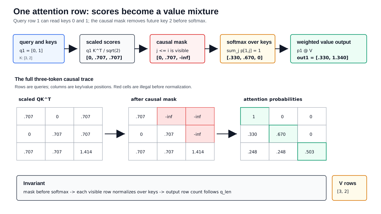
The corresponding executable trace is deliberately literal:
q = torch.tensor([[1.0, 0.0], [0.0, 1.0], [1.0, 1.0]])
k = q.clone()
v = torch.tensor([[1.0, 0.0], [0.0, 2.0], [1.0, 1.0]])

scores = q @ k.T / math.sqrt(q.size(-1))
causal = torch.tril(torch.ones(3, 3, dtype=torch.bool))
masked_scores = scores.masked_fill(~causal, -float("inf"))
p_attn = masked_scores.softmax(dim=-1)
out = p_attn @ v
This one example exposes four independent audit points: the transpose creates query-by-key scores, scaling changes their magnitude, masking changes which columns participate in normalization, and the final multiplication moves from key-space weights back into value-space vectors.
The source figure writes one causal head row rather than a full batch. It makes the same ownership visible: the current row supplies the query, allowed prefix rows supply keys and values, and the output is a value-space mixture.
0x09B An auditable eager implementation
A reference implementation should expose semantic checks, not only return a tensor with the expected rank:
def eager_attention(
    q, k, v, visible=None, bias=None, dropout_p=0.0, training=False,
    dropout_multiplier=None,
):
    # q: [B,H,Q,D], k: [B,H,K,D], v: [B,H,K,Dv]
    assert q.ndim == k.ndim == v.ndim == 4
    assert q.shape[:2] == k.shape[:2] == v.shape[:2]
    assert q.shape[-1] == k.shape[-1]
    assert k.shape[-2] == v.shape[-2]

    scores = q @ k.transpose(-2, -1)
    scores = scores * (q.shape[-1] ** -0.5)

    if bias is not None:
        scores = scores + bias.to(device=scores.device, dtype=scores.dtype)

    if visible is not None:
        visible = visible.to(device=scores.device, dtype=torch.bool)
        visible = torch.broadcast_to(visible, scores.shape)
        assert visible.any(dim=-1).all(), "every used query needs a legal key"
        scores = scores.masked_fill(~visible, -torch.inf)

    pre_dropout = torch.softmax(scores, dim=-1, dtype=torch.float32)
    pre_dropout = pre_dropout.to(q.dtype)

    if dropout_multiplier is not None:
        # Test/oracle path: replay one already-sampled coordinate-wise Z.
        assert training and dropout_multiplier.shape == pre_dropout.shape
        consumed = pre_dropout * dropout_multiplier.to(pre_dropout.dtype)
    else:
        consumed = torch.dropout(pre_dropout, dropout_p, training)

    output = consumed @ v

    assert output.shape == (*q.shape[:-1], v.shape[-1])
    if not training or dropout_p == 0.0:
        row_sum = pre_dropout.float().sum(dim=-1)
        torch.testing.assert_close(row_sum, torch.ones_like(row_sum))
    return output, {
        "pre_dropout": pre_dropout,   # normalized distribution P
        "consumed": consumed,         # stochastic weights Pdrop
    }
The row-sum assertion is conditional because dropout on probabilities changes
the realized row sum during training. Dropout is unbiased in expectation after
its rescaling; one sampled mask does not remain a normalized probability row.
That is another reason not to inspect post-dropout p_attn and assume it is the
same object as pre-dropout routing probabilities.
The optional dropout_multiplier is an oracle hook, not a proposed public API.
A production eager path normally asks the framework dropout operator to sample
Z; a conformance test needs a way to replay one fixed realization across
manual, autograd, and finite-difference calculations.
Derivation The backward pass of this function under a fixed dropout mask (gradients for V, the probabilities, the scores, Q and K), a finite-difference check, why masked and dropped edges differ, and the projection-weight gradients; open it when implementing or debugging backward. (about 680 words, 6 code listings, 22 equations)
Backward path: every role receives a different signal
Backward differentiates the exact sampled forward program. Hold Z fixed and
write:
The value matmul sends gradients down two branches. Its value gradient is weighted by the consumed stochastic matrix:
The gradient of the consumed weights is:
The fixed dropout multiplier then gates the direct probability gradient:
Dropout does not create a differentiable path into the sampled Bernoulli
decision. Conventional attention dropout treats Z as realized training
input. If a method learns a drop rate or a discrete gate with another
estimator, that is a different optimization contract.
Softmax couples every legal score in one query row. Define the row contraction:
Substituting the preceding branches gives a second form that is useful in fused backward algorithms:
The softmax gradient is then:
For S=alpha QK^T, with alpha=1/sqrt(d_k), the score matmul returns:
The scale appears once in both branches. Omitting it, or applying it again
inside G_S, can preserve all shapes while changing every Q/K gradient.
Fixed-mask backward trace
For the forward fixture above, freeze:
G_O = [[ 0.7, -0.4],
       [-0.2,  0.9]]
The two equivalent row contractions and the resulting score gradient are:
D from sum(P * G_P) = [1.105096, 2.072873]
D from sum(G_O * O) = [1.105096, 2.072873]

G_S =
  [[ 0.272434, -0.272434,  0.000000],
   [-0.532981, -0.383297,  0.916279]]
The maximum central-finite-difference error over Q, K, and V is
2.84e-10 in float64 with epsilon 1e-6. Reconstructing P from saved
row log-sum-exp differs by at most 2.78e-17, and replaying the same Z
changes the manual gradients by at most 1.11e-16. Drawing the fixture’s
different fresh mask instead produces a maximum gradient mismatch of
0.771809. That is not stochastic tolerance; it is differentiation of a
different program.
Dropped, masked, and all-dropped routes have different gradients
The fixed trace exposes a subtle consequence of softmax coupling:
legal edge (query 0, key 1) is dropped:
    Z[0,1] = 0
    direct G_P[0,1] = 0
    score G_S[0,1] = -0.272434   # generally nonzero

illegal edge (query 0, key 2) is masked:
    P[0,2] = 0
    score G_S[0,2] = 0
The dropped edge receives no direct gradient through its own consumed route, but its score still affects the softmax denominator that allocated pre-dropout mass to kept edges. A masked edge is absent from that denominator and has zero ideal score gradient.
If every legal edge in one row drops, then Pdrop_i=0 and O_i=0. For that
row, the contributions to G_V, G_P, D_i, G_S, G_Q, and G_K are
all zero. This well-defined stochastic event is different from asking
softmax to normalize an empty legal support. The oracle checks both
distinctions and also verifies:
sum_j G_S[i,j] = 0 for each legal finite row
masked G_S entries = 0
all-dropped row attention gradients = 0
This exposes the training semantics that the forward mnemonic hides:
V learns what payload helps the downstream loss.
Q learns what each output row should request.
K learns how each memory row should advertise itself.
An additive mask with true -inf gives blocked entries zero probability; their
score gradients are correspondingly zero under the ideal softmax semantics.
This does not mean a padded token can never receive gradients elsewhere in the
network. Residual paths, embeddings, losses, and query-side computation have
their own masking contracts.
Projection gradients reconnect the local attention call to the model
M3.1 receives projected tensors, but training eventually updates the projection weights owned by M3.2. If:
then:
Input-state gradients accumulate all roles in self-attention because the same
X feeds Q, K, and V:
In cross-attention, target states receive the Q branch while source memory receives the K and V branches. This is the backward counterpart of the forward stream contract:
self-attention:
    one state stream receives Q + K + V gradient contributions

cross-attention:
    target stream receives Q contribution
    source-memory stream receives K + V contributions
The split matters when freezing an encoder, reusing source memory, adding adapters to selected projections, or debugging a detached memory tensor.
0x09C Reference semantics versus production attention APIs
One mathematical attention call can appear as several code paths. The correct comparison is not line count; it is which semantic objects each path accepts, returns, saves for backward, or fuses.
Path 1: explicit eager attention
The eager_attention function above materializes scores and probabilities.
Advantages:
every intermediate can be inspected;
custom finite bias and visibility are explicit;
attention probabilities can be returned;
gradient checks can target each stage.
Costs:
score and probability tensors may occupy O(B*H*Q*K) memory;
separate kernels move intermediates through memory;
Python/model code must handle mask polarity and all-masked rows.
This is the conformance oracle, not necessarily the production backend.
Path 2: functional scaled dot-product attention
PyTorch exposes the local operation directly:
def sdpa_attention(q, k, v, visible=None, dropout_p=0.0, training=False):
    additive = None
    if visible is not None:
        visible = torch.broadcast_to(visible, (*q.shape[:-2], q.size(-2), k.size(-2)))
        assert visible.any(dim=-1).all()
        additive = torch.zeros_like(visible, dtype=q.dtype)
        additive = additive.masked_fill(~visible, -torch.inf)

    return torch.nn.functional.scaled_dot_product_attention(
        q,
        k,
        v,
        attn_mask=additive,
        dropout_p=dropout_p if training else 0.0,
        is_causal=False,
    )
The explicit training branch is important: the functional API uses the
provided dropout_p; it does not inspect a module’s .training flag for the
caller. The example sets is_causal=False because visibility has already been
encoded. Passing both a custom mask and an implicit causal contract requires
checking the exact framework version and backend behavior rather than assuming
they compose identically.
An implementation may dispatch to math, memory-efficient, or Flash-style backends. Dispatch can depend on device, dtype, dimensions, mask form, dropout, and whether gradients or attention weights are requested. Backend selection is not part of the checkpoint’s learned function, but it is part of reproducible execution.
Path 3: model-integrated attention
A decoder layer usually wraps the local operation with additional state:
q = q_proj(hidden_states)
k = k_proj(key_value_states)
v = v_proj(key_value_states)

q, k, v = split_heads(q, k, v)
q, k = apply_position_geometry(q, k, position_ids)
k, v = cache.update(k, v, cache_position)

out = scaled_dot_product_attention(q, k, v, ...)
out = merge_heads(out)
out = o_proj(out)
M3.1 owns only the middle score path, but a local test must still verify what arrives there:
Q/K already use the intended position transform;
K/V contain exactly the legal cached rows;
query and cache positions describe the same coordinate system;
mask dimensions refer to the post-cache key length;
dtype/device match the selected backend.
The A10 implementation diagram separates the same five local operations: score matmul, scale, optional mask, softmax, and value matmul.
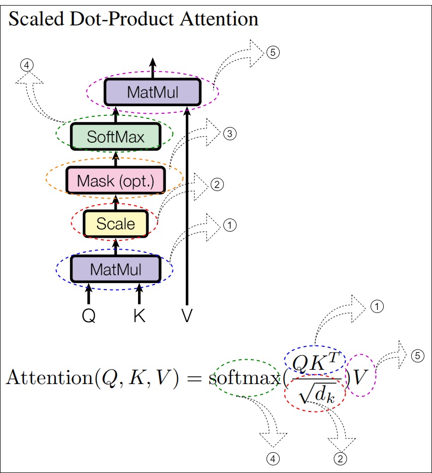
Implementation and runtime contracts Why requesting attention weights can change the execution path, why an attention map alone is not an explanation, and what dense, recomputing and fused paths save for backward; open it before profiling or interpreting attention maps. (about 490 words, 2 code listings, 2 equations, 1 figure)
Requesting attention weights can change the execution path
An optimized kernel can produce O without writing the full P matrix to
HBM. Asking for all attention weights may therefore:
force an eager or different backend;
materialize B*H*Q*K elements;
increase backward saved state;
change latency enough to invalidate a benchmark;
still return a tensor that is unsuitable as a causal explanation.
Debug runs should state whether weights are pre-dropout or post-dropout and whether they came from the same backend as normal execution. Production profiling should normally disable weight return unless the feature itself is a requirement.
PyTorch MultiheadAttention documents need_weights=False as the path that
permits its optimized SDPA implementation. That is an API performance
contract, not a mathematical statement that P does not exist. Conversely,
a returned tensor named attn_weights does not by itself prove whether it is
P, Pdrop, head-averaged P, or a tensor recomputed by another backend.
The wrapper contract must say which object it returns.
An attention map is also only one part of the head function. Jain and Wallace
showed counterexamples to treating learned attention weights as explanations;
Wiegreffe and Pinter argued that stronger, task- and definition-specific tests
can still make attention analytically useful. The bounded conclusion here is
not that attention weights are meaningless. It is that a routing matrix alone
omits V, W_O, residual state, downstream nonlinearities, and counterfactual
behavior, so it must not be labeled a causal explanation without an explicit
method and validation contract.
Training state saved by the local operation
Backward needs enough state to recover Q, K, V, the pre-dropout probability, and the exact sampled dropout multiplier. It does not require every one of those objects to be stored as a dense tensor. The saved-state choice is a time-memory-reproducibility contract:
| Path | Typical forward-visible state | Sufficient backward state | Backward work | Main failure |
|---|---|---|---|---|
| explicit eager | materialized S, P, Pdrop, O | framework-dependent Q/K/V plus retained P and mask/multiplier | dense matmuls and softmax backward | silently retaining quadratic tensors beyond their useful lifetime |
| checkpoint/recompute | often only O visible | Q/K/V, visibility/bias, scale, dropout replay state, normalization statistics or inputs | recreate scores/probabilities, then contract gradients | replaying another mask or another model state |
| fused IO-aware | no global S or P required | Q/K/V, O, row log-normalizers, coordinate-stable RNG state, kernel metadata | tile-local score/probability recomputation | tile-order-dependent RNG or wrong gradient ownership |
One dense reconstruction route saves the row log-partition L_i and recomputes:
on legal entries. The Loop 6 oracle reconstructs the fixture probabilities
with maximum error 2.78e-17. It then replays the fixed coordinate-wise
dropout multiplier and reproduces the analytic gradients within 1.11e-16.
Those are semantic conformance checks, not expected low-precision GPU
tolerances.

The visual is reused at a different level of abstraction. M3.1 derives the dense operation that must be preserved. M4.3 owns the FlashAttention tile schedule, HBM/SRAM traffic, recomputation order, and gradient-write ownership.
This creates a three-way distinction:
forward mathematical state:
    Q, K, V -> exact output O

debug-visible state:
    optional full scores or probabilities

autograd saved state:
    backend-specific tensors/statistics needed for backward
Conflating them leads to claims such as “attention requires storing the full matrix” or “FlashAttention has no attention probabilities.” The mathematical probabilities exist; whether they are materialized, returned, or recomputed is an execution choice.
How this was checked A table of dropout and backward mistakes with how each is detected, and the commands the article's test code runs for this part; open it when debugging attention during training. (about 260 words, 2 code listings)
Loop 6 failure lab
| Failure | Shape-valid symptom | Broken invariant | Detection |
|---|---|---|---|
| assert post-dropout rows sum to one | intermittent training assertion | only pre-dropout P is normalized | compare sum(P) and realized sum(Pdrop) separately |
| sample a fresh mask in backward | noisy, irreproducible gradients | backward differentiates a different program | fixed-mask replay parity test |
use Pdrop in the softmax Jacobian | plausible but wrong Q/K gradients | softmax produced P, then dropout produced Pdrop | float64 finite difference against fixed Z |
omit Z from G_P | dropped routes receive direct gradient | chain rule through Pdrop=P*Z is missing | inspect a dropped legal edge |
use P instead of Pdrop in G_V | value gradient ignores sampled routing | forward consumed Pdrop@V | manual/autograd V-gradient parity |
| treat dropped edge as masked edge | force G_S=0 at a dropped legal score | legal edge still participates in softmax denominator | inspect fixed edge (0,1) |
| treat all-dropped row as all-masked row | reject a valid dropout sample or create NaNs | support is nonempty even when all sampled routes drop | separate legal-count and keep-count assertions |
omit alpha in Q/K backward | gradients have correct shapes and wrong scale | S=alpha QK^T | scale-ratio and finite-difference checks |
| leave functional SDPA dropout active in evaluation | nondeterministic evaluation outputs | functional API obeys dropout_p, not module mode | repeated eval call and explicit dropout_p=0.0 |
| request weights during benchmark | latency and memory regress unexpectedly | return contract changes dispatch/materialization | record backend and need_weights in run manifest |
Loop 6 executable gate
The evidence package turns this section into executable claims:
cd docs/numinens-evidence/m3-1-attention-score-path
python3 loop6_attention_oracle.py
python3 loop6_contract_audit.py
python3 -m unittest -v test_loop6_contract
Publication requires all of the following:
analytic and Monte Carlo dropout moments agree within declared tolerances;
fixed-mask manual Q/K/V gradients pass central finite differences;
the two D_i contractions agree;
masked, dropped, and all-dropped cases remain distinct;
same-mask replay agrees and fresh-mask replay demonstrably fails;
alternative renormalization is not mislabeled as unbiased inverted dropout;
source and visual provenance resolve locally;
Loops 1-5 section hashes remain frozen.
0x0A Self-attention, causal self-attention, and cross-attention axes
The same score path covers several attention calls.
| Mode | Query source | Key/value source | Score shape | Mask object |
|---|---|---|---|---|
| Encoder self-attention | encoder states | encoder states | [B,h,S,S] | source padding mask |
| Decoder causal self-attention | target/prefix states | target/prefix states | [B,h,T,T] | causal + target padding mask |
| Cross-attention | decoder states | encoder memory | [B,h,T,S] | source memory padding mask |
| One-token decode boundary | current token state | cached history + current key/value | [B,h,1,past+1] | cache-aware visibility mask |
The local math is identical. The axes change.
Cross-attention is the easiest shape trap. Its score object is target-by-source:
scores: [B, h, T, S]
Applying a target causal mask to cross-attention because the tensor happens to be rank four is a semantic error. Source keys are not future target tokens.
0x0A1 Full Source-to-Tensor and Eager Implementation Trace
The three-token example in 0x09A traced one call by hand. This section repeats the exercise for a cross-attention call in which two target rows read three source rows, one of them padding, and records every intermediate value; the stages and the matching reference code are folded below.
The earlier sections isolated each mathematical stage. This section asks a different implementation question:
Given one concrete caller, can we name the source row behind every tensor axis, reproduce every intermediate value, and explain every difference between the compact Harvard function and a defensive eager reference?
That question is stricter than checking the final shape. Many attention bugs
preserve [B,H,Q,Dv]: K and V can be permuted differently, a source mask can
be aligned to the query axis, softmax can reduce the wrong dimension, or a
finite bias can revive an edge if support exclusion is applied in the wrong
order. A full trace gives those errors nowhere to hide.
How this was checked How the trace keeps the source description, the equation and the program in agreement, and why it runs in evaluation mode; open it for the setup of the trace. (about 60 words, 1 code listing)
Loop 7 contract: reconcile source, equation, and program
Loop 7 freezes three descriptions of one operation:
source description:
    target rows query an encoder/source memory;
    source row j owns both key j and value j;
    source validity determines which memory rows are legal

equation description:
    S = alpha Q K^T
    S_bias = S + B
    S_mask = where(visible, S_bias, -inf)
    P = softmax_K(S_mask)
    O = (P * Z) V

program description:
    explicit tensors, views, broadcast adapters, work dtype,
    saved trace objects, assertions, and return semantics
The three must agree on row identity, not only dimensions. The fixture runs in
evaluation mode, so its dropout multiplier is Z=1. Loop 6 already owns the
stochastic training derivation and backward replay. Loop 7 records where that
multiplier would enter the complete forward program without reopening its
statistics.
The caller boundary is part of the trace, not part of the local owner
The original Transformer separates scaled dot-product attention from the multi-head wrapper:
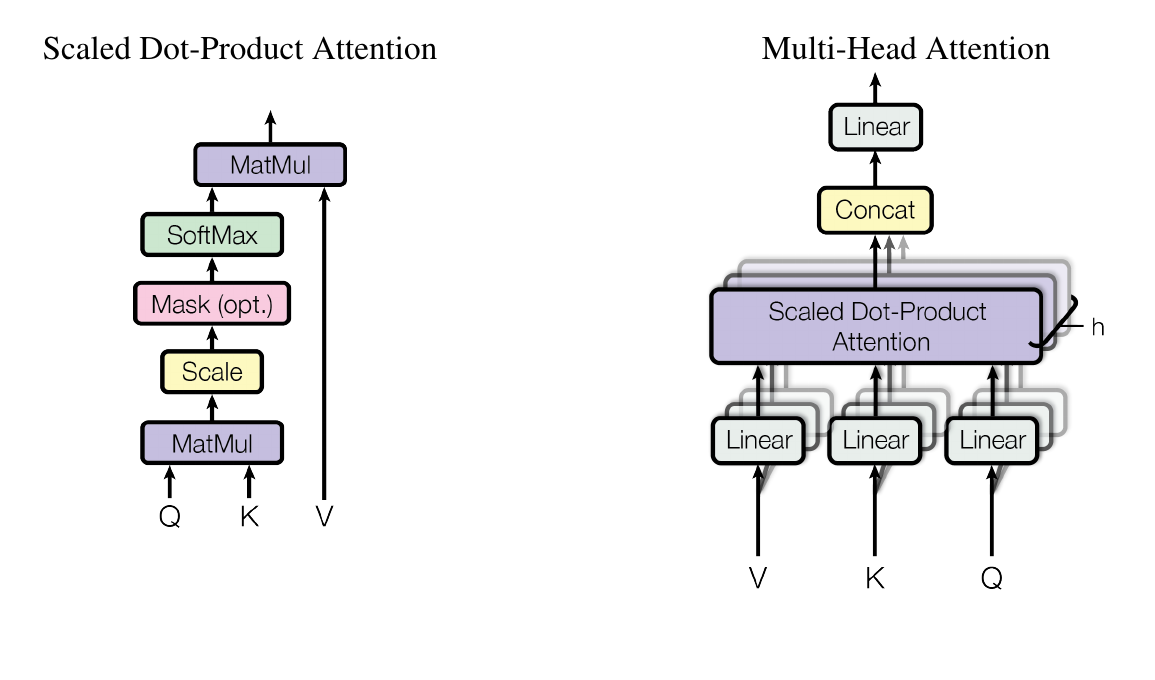
Source: Attention Is All You Need, Figure 2. The left panel is M3.1’s local owner. The right panel is the M3.2 caller. Showing both is necessary for lineage; it does not transfer projection, head split, concatenation, or W_O ownership into this article.
Implementation and runtime contracts Which stages belong to the caller (projections, head merge) and which to this call, and a line-by-line comparison of the compact Harvard function with a safer reference; open it before reading the trace. (about 550 words, 1 code listing)
Use the following firewall when reading the executable fixture:
| Stage | Concrete object | Owner in Transformer System | Loop 7 use |
|---|---|---|---|
| data identity | target/source token IDs, padding/segment metadata | M2.1 | retain row provenance; do not derive tokenization |
| vector state | target hidden rows and encoder/source memory rows | M2.2 and earlier blocks | provide deterministic caller inputs |
| learned adapters | W_Q, W_K, W_V, head split, head map | M3.2 | expose the exact Q/K/V values received by M3.1 |
| local attention | score, scale, finite bias, visibility, normalization, dropout, value mix | M3.1 | derive and execute every intermediate |
| assembled result | head merge, W_O, residual branch | M3.2 and M3.7 | consume per-head O; remain outside this fixture |
The trace therefore starts before the M3.1 API only to prove lineage. Its
projection matrices use equation orientation [Dmodel,Dout], so row vectors
compute X @ W. A PyTorch nn.Linear checkpoint stores its weight in
[Dout,Din]; M3.2 owns that orientation conversion.
The Harvard source and the safe reference have different jobs
A10 and A11 reconstruct the compact function from the Annotated Transformer:
d_k = query.size(-1)
scores = torch.matmul(query, key.transpose(-2, -1)) / math.sqrt(d_k)
if mask is not None:
    scores = scores.masked_fill(mask == 0, -1e9)
p_attn = scores.softmax(dim=-1)
if dropout is not None:
    p_attn = dropout(p_attn)
return torch.matmul(p_attn, value), p_attn
That code is an excellent equation spine. It is not a complete execution manifest. A defensive oracle makes assumptions explicit:
| Harvard line | Preserved meaning | Safe-reference addition |
|---|---|---|
query.size(-1) | Q/K score width owns 1/sqrt(Dk) | assert Q and K widths agree; record alpha |
key.transpose(-2,-1) | exchange K’s row and feature axes | record shape/stride and keep key/value row IDs paired |
torch.matmul | batch/head axes are batch dimensions | reject unintended Q/K/V broadcasting before calling it |
/ sqrt(d_k) | scale every compatibility logit once | record configured multiplier; detect double scaling |
masked_fill(mask == 0, -1e9) | illegal keys leave the distribution | adapt canonical True=legal; use -inf; reject empty used rows |
softmax(dim=-1) | normalize over source/key rows | expose max, shifted logits, exponentials, and denominator in work dtype |
dropout(p_attn) | sample consumed routing weights | retain both pre-dropout P and consumed Pdrop; record replay state |
p_attn @ value | mix value rows with key-axis weights | assert K rows equal V rows and preserve source row identity |
return p_attn | expose the function’s current weight object | name whether returned weights are pre- or post-dropout |
PyTorch’s torch.matmul
broadcasts its leading batch dimensions. That behavior is useful, but it can
hide a missing head or batch axis. The safe oracle requires Q/K/V leading axes
to match exactly and permits broadcasting only for declared metadata such as
visibility and finite bias. PyTorch’s
broadcasting rules
align trailing dimensions; they do not know that one axis means head and
another means query.
The broad A11 reconstruction is useful because it shows the complete source path in one surface:
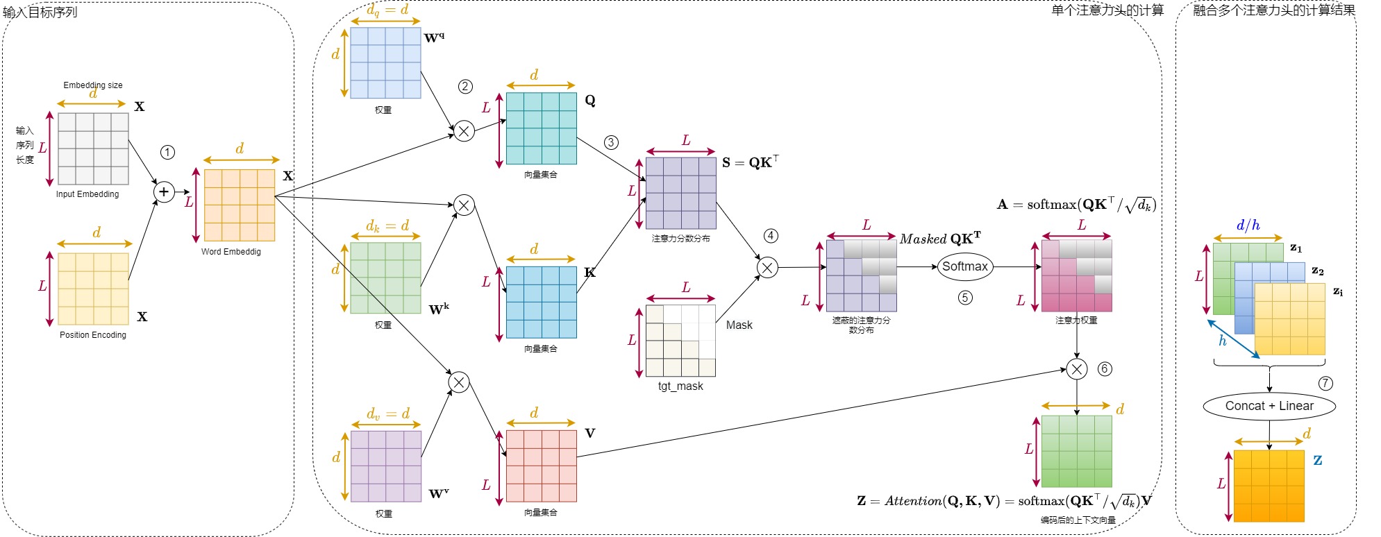
Source-local A11 figure. Read it critically: input/position construction is upstream, projections and multi-head merge belong to M3.2, and the multiplication symbol drawn between the score matrix and mask is schematic. Authoritative visibility is not score multiplication; it is support exclusion before softmax, as derived in Loop 4.
Worked detail The cross-attention call traced stage by stage (projection, scores, a large bias on the padded row, masking, stable softmax, value mixing), showing that the mask beats any finite bias; open it for a second complete numerical example. (about 480 words, 4 code listings, 30 equations)
Fixed fixture: two target rows read three source rows
The fixture is a one-batch, one-head cross-attention call:
B=1, H=1, Q=2, K=3, Dmodel=3, Dk=2, Dv=2
target token IDs: [31, 47]
source token IDs: [11, 22, PAD]
source row IDs:   [source:0, source:1, source:2]
Token IDs are provenance labels, not arithmetic inputs to M3.1. Upstream
embedding/block computation supplies target states Xq and source memory
Xm:
The caller’s deterministic projection matrices are:
Stage 1: project and expose the head axis
The M3.2 caller computes:
After adding batch and head axes:
Q: [1,1,2,2]
K: [1,1,3,2]
V: [1,1,3,2]
Key row j and value row j still name the same source row. That paired-row
invariant is more important than the coincidence Dk=Dv=2 in this fixture.
Permuting K without applying the same source-row permutation to V leaves every
matrix multiplication shape-valid and changes the retrieved content.
Stage 2: transpose the key view and compute compatibility
K.transpose(-2,-1) is a logical [1,1,2,3] view. The batched product is:
With alpha=1/sqrt(2)=0.70710678:
The output row axis comes from Q and the column axis comes from K. This is why
the result is target-by-source [2,3], not a square matrix inferred from tensor
rank.
Stage 3: add finite preference, then enforce source visibility
Use a query-specific finite bias:
The padded source row deliberately receives +7. This turns operation order
into an executable test: no finite preference may revive an illegal edge.
The semantic visibility object begins as a source-row vector:
source_visible: [True, True, False]      shape [B,K] = [1,3]
visible:        [True, True, False]      shape [B,1,1,K] = [1,1,1,3]
broadcast view: two identical query rows shape [B,H,Q,K] = [1,1,2,3]
After bias:
After authoritative support exclusion:
The large third-column bias remains observable in biased_scores for audit,
but it cannot enter the denominator.
Stage 4: expose the stable-softmax state
The legal row maxima are:
Subtracting them and exponentiating legal entries gives:
with denominators:
Therefore:
The fixture uses float64 so the published values and executable oracle can
agree tightly. A production eager call may use float32 for the softmax work
state and cast probabilities back. The torch.softmax
dtype parameter makes that policy explicit; fused kernels may preserve the
same mathematical row through a different internal schedule.
Stage 5: consume probabilities and mix source values
Evaluation mode fixes:
The per-head output is:
For the first target row:
0.3650 * value(source:0) + 0.6350 * value(source:1)
= 0.3650 * [1, 2]       + 0.6350 * [2, -1]
= [1.6350, 0.0951]
value(source:2) contributes exactly zero. The reason is semantic exclusion,
not a small score and not attention dropout.
Code and tensors Every intermediate with its shape and value, a traceable reference implementation, how source-row identity survives each step, how self-, cross- and cached attention differ only in their inputs, and stage-by-stage assertions; open it when instrumenting your own attention code. (about 690 words, 5 code listings)
Every intermediate has both values and execution metadata
The complete local ledger is:
| Object | Shape | Value summary | Storage/materialization statement |
|---|---|---|---|
q | [1,1,2,2] | [[2,1],[1,2]] | caller-produced head view or tensor |
k | [1,1,3,2] | three source key rows | caller-produced; row-aligned with V |
v | [1,1,3,2] | three source payload rows | caller-produced; row-aligned with K |
k_t | [1,1,2,3] | same K values, axes exchanged | transpose view; no semantic row reorder |
dot | [1,1,2,3] | [[3,3.5,2.5],[3,2.5,3.5]] | materialized by this eager oracle |
scaled | [1,1,2,3] | dot / sqrt(2) | one configured scale |
bias_effective | [1,1,2,3] | query-specific, including illegal +7 | broadcast view when caller supplies fewer axes |
visible_effective | [1,1,2,3] | third source column false | broadcast view; semantic True=legal |
masked_scores | [1,1,2,3] | third column -inf | authoritative support encoding |
row_max | [1,1,2,1] | [2.6749,2.1213] | reduction work state |
exp_shifted | [1,1,2,3] | masked column exactly zero | normalization work state |
denominator | [1,1,2,1] | [1.5749,1.6354] | strictly positive used-row state |
pre_dropout | [1,1,2,3] | rows sum to one | semantic probability object |
dropout_multiplier | [1,1,2,3] | all ones in this eval fixture | training would require sampled replay state |
consumed | [1,1,2,3] | equals P in evaluation | weights actually passed to V mix |
output | [1,1,2,2] | two target-indexed value mixtures | M3.1 return to M3.2 caller |
Full matrices belong in a tiny oracle trace, not in production telemetry. A runtime manifest normally records shape, dtype, device, stride, contiguity, materialization policy, and small checksums/statistics. Dumping attention matrices for real batches changes memory lifetime, may expose sensitive token relationships, and can force a different backend.
A traceable safe eager reference
The following function is intentionally more verbose than the code spine. It is a semantic oracle and debugging instrument, not the recommended production kernel:
def eager_attention_trace(
    q, k, v, *, visible, bias=None,
    dropout_multiplier=None, softmax_dtype=torch.float32,
):
    # Local contract: already projected/head-shaped tensors.
    assert q.ndim == k.ndim == v.ndim == 4
    assert q.shape[:2] == k.shape[:2] == v.shape[:2]
    assert q.shape[-1] == k.shape[-1]
    assert k.shape[-2] == v.shape[-2]
    assert q.device == k.device == v.device

    B, H, Q, Dk = q.shape
    K, Dv = k.shape[-2], v.shape[-1]
    expected_scores = (B, H, Q, K)
    trace = {"q": q, "k": k, "v": v}

    k_t = k.transpose(-2, -1)
    dot = torch.matmul(q, k_t)
    alpha = Dk ** -0.5
    scaled = dot * alpha

    if bias is None:
        bias_effective = torch.zeros_like(scaled)
    else:
        bias = bias.to(device=scaled.device, dtype=scaled.dtype)
        bias_effective = torch.broadcast_to(bias, expected_scores)
    biased = scaled + bias_effective

    visible = visible.to(device=scaled.device, dtype=torch.bool)
    visible_effective = torch.broadcast_to(visible, expected_scores)
    if not visible_effective.any(dim=-1).all():
        raise ValueError("every consumed query row needs at least one legal key")
    masked = biased.masked_fill(~visible_effective, -torch.inf)

    work = masked.to(softmax_dtype)
    row_max = work.max(dim=-1, keepdim=True).values
    shifted = work - row_max
    exp_shifted = torch.where(
        visible_effective, torch.exp(shifted), torch.zeros_like(shifted)
    )
    denominator = exp_shifted.sum(dim=-1, keepdim=True)
    pre_dropout_work = exp_shifted / denominator
    pre_dropout = pre_dropout_work.to(v.dtype)

    if dropout_multiplier is None:
        dropout_multiplier = torch.ones_like(pre_dropout)
    else:
        assert dropout_multiplier.shape == expected_scores
        dropout_multiplier = dropout_multiplier.to(
            device=pre_dropout.device, dtype=pre_dropout.dtype
        )
    consumed = pre_dropout * dropout_multiplier
    output = torch.matmul(consumed, v)

    trace.update({
        "k_t": k_t,
        "dot": dot,
        "alpha": alpha,
        "scaled": scaled,
        "bias_effective": bias_effective,
        "biased_scores": biased,
        "visible_effective": visible_effective,
        "masked_scores": masked,
        "row_max": row_max,
        "shifted": shifted,
        "exp_shifted": exp_shifted,
        "denominator": denominator,
        "pre_dropout": pre_dropout,
        "dropout_multiplier": dropout_multiplier,
        "consumed": consumed,
        "output": output,
    })
    assert output.shape == (B, H, Q, Dv)
    return output, trace
Two choices are deliberate.
First, Q/K/V do not broadcast. torch.matmul could broadcast leading axes,
but a safe reference rejects that convenience because physical head mapping is
an M3.2 decision. Visibility and finite bias may broadcast because their
manifests explicitly declare that behavior.
Second, torch.broadcast_to returns an expanded view. A broadcast head/query
axis can have stride zero: several logical coordinates name the same storage.
The trace never mutates bias_effective or visible_effective in place. A
later implementation that writes through an expanded view is not equivalent to
reading broadcast metadata.
Source identity survives every legal transformation
An end-to-end debugger should carry row labels beside tensor values:
query row labels:
    [target:0, target:1]

key/value row labels:
    [source:0, source:1, source:2]

score cell [i,j]:
    compatibility(target:i, source:j)

probability cell [i,j]:
    normalized legal routing weight from target:i to source:j

output row [i]:
    mixture of source value rows for target:i
Transpose does not reorder source identities; it changes how K participates in the matrix product. Broadcasting the source mask does not create new source rows; it applies one source-validity decision to several heads/query rows. Softmax does not move identities; it normalizes each fixed query row over the key axis. Value mixing removes the key axis by contracting each probability column with the correspondingly indexed value row.
This yields a useful conservation rule:
before P @ V:
    key axis j and value row j must denote the same source object

after P @ V:
    key axis is contracted away;
    query row identity and value feature identity remain
The rule catches a data-pipeline bug that pure tensor algebra cannot: if K is sorted, sharded, cached, or gathered under one index map and V under another, the calculation is numerically valid and semantically corrupt.
Self-attention, cross-attention, and cached self-attention are caller variants
The safe function does not branch on an attention_type string. The caller
creates different source objects and coordinates:
| Call | Q lineage | K/V lineage | Typical shape | Visibility owner |
|---|---|---|---|---|
| full self-attention | current stream, all query rows | same stream, same represented rows | [B,H,S,S] | bidirectional or causal/padding policy |
| rectangular cross-attention | target stream | encoder/source memory | [B,H,T,S] | source validity; normally no target causal triangle |
| cached one-token self-attention | current row | prior cached rows plus current row | [B,H,1,past+1] | cache coordinates and chronology |
| chunked cached self-attention | several current rows | cache prefix plus current chunk | [B,H,Qchunk,past+Qchunk] | absolute query/key coordinates |
The full numeric fixture is cross-attention because Q=2 and K=3 make axis
ownership visible. A rectangular cached-self call can have the same score
shape while representing a different graph. Shape does not determine whether
the source is encoder memory or history from the same stream.
Reconciliation assertions
The fixture checks values at stage boundaries rather than trusting only the final output:
output, t = eager_attention_trace(...)

assert t["k_t"].shape == (1, 1, 2, 3)
assert t["dot"].shape == (1, 1, 2, 3)
assert t["visible_effective"].shape == t["dot"].shape
assert torch.isneginf(t["masked_scores"][..., 2]).all()
assert (t["pre_dropout"][..., 2] == 0).all()
torch.testing.assert_close(
    t["pre_dropout"].sum(dim=-1),
    torch.ones((1, 1, 2), dtype=t["pre_dropout"].dtype),
)
torch.testing.assert_close(output, t["consumed"] @ t["v"])
The evidence oracle additionally compares:
vectorized safe trace
    == scalar row-by-row reference
    == Harvard-style translated-mask reference

output row i
    == sum_j probability[i,j] * value[j]

masked source column
    == zero probability and zero value contribution
The Harvard comparison is restricted to its shared contract: one head-shaped
Q/K/V call, no empty legal row, the same finite bias inserted before its mask
step, dropout disabled, and 1=legal/0=blocked mask adaptation. Agreement does
not prove that -1e9 is a universal mask policy or that implicit dtype/backend
choices are safe.
How this was checked A table of shape-preserving mistakes this trace catches, and the commands the article's test code runs for it; open it when choosing debugging tests. (about 280 words, 2 code listings)
Loop 7 failure lab
| Failure | Why the final shape can still pass | Broken trace invariant | Detection |
|---|---|---|---|
| permute K without V | both remain [B,H,K,D] | key row j no longer addresses value row j | row-ID manifest plus scalar weighted-sum oracle |
| normalize over query axis | softmax returns the same rank | each source column competes across queries | assert row sums over K, not column sums over Q |
align [B,Q,K] mask as if it were [B,1,Q,K] | dimensions may accidentally agree when B=H | batch identity is consumed as head identity | canonicalize named axes before broadcasting |
| add finite bias after masking | a large finite value can replace/revive exclusion under a faulty encoding | support must dominate preference | fixture’s illegal +7 column remains zero probability |
| squeeze batch/head axes in a toy | B=H=1 numeric result looks right | general batched/head contract is lost | keep rank-four assertions in the oracle |
| transpose V like K | dimensions may pass when K=Dv | P contracts with the value feature axis | source-row weighted-sum check |
| silently broadcast Q/K/V heads | torch.matmul permits leading-axis broadcast | physical head ownership changes | require identical Q/K/V leading axes |
| mutate a broadcast mask view | repeated logical rows may alias storage | metadata adaptation changes another row | read-only expanded view and no in-place operations |
| return only one unnamed weight tensor | caller cannot tell P from Pdrop | interpretation and backward state become ambiguous | named pre_dropout and consumed fields |
| validate only final output | compensating bugs can cancel in one fixture | no stage-level reconciliation | freeze intermediate shapes and values |
Loop 7 executable gate
The deterministic evidence package runs the full fixture and freezes the source/visual contract:
cd docs/numinens-evidence/m3-1-attention-score-path
python3 loop7_source_to_tensor_oracle.py
python3 loop7_contract_audit.py
python3 -m unittest -v test_loop7_contract
Publication requires:
every projected row retains target/source provenance;
every intermediate shape and numeric value matches the fixture;
vectorized, scalar, and Harvard-style references agree;
the illegal high-bias source row remains excluded;
K/V row permutations fail the semantic oracle despite valid shapes;
only declared metadata broadcasts;
the M3.1/M3.2 ownership firewall remains explicit;
Loops 1-6 section hashes remain frozen.
0x0A2 SDPA, Framework, and Model Runtime Integration
This section follows the same call into PyTorch’s scaled_dot_product_attention, nn.MultiheadAttention and Hugging Face model code: mask polarity, causal alignment for cached calls, grouped-query heads, dropout in evaluation mode, backend selection, and tests that compare eager and fused paths. Open it when you move from the reference function to a framework call.
Implementation and runtime contracts Why framework paths that implement the same equation can still disagree on mask polarity, causal alignment, dropout mode, grouped heads, returned weights or backend. (about 120 words)
Loop 7 ended with a defensive eager function whose intermediate values can be inspected. Production models rarely call that function directly. They project and position Q/K/V, adapt a semantic visibility relation to a framework API, ask a dispatcher for an eligible implementation, and return only the objects the caller requested.
That indirection is useful, but it creates a new class of bugs. Two runtime paths may implement the same equation while disagreeing about boolean polarity, causal alignment, dropout mode, GQA head mapping, returned weights, or whether a requested backend actually ran.
Owner question. How does the exact eager operation from Loop 7 cross a framework and model-runtime boundary without allowing API defaults or backend dispatch to redefine its support, scale, stochastic state, or output meaning?
How this was checked The four runtime layers kept apart here (semantic operation, API adapter, dispatcher, model runtime) and the framework versions the claims are tied to. (about 260 words, 1 code listing)
Loop 8 contract: preserve semantics across four runtime layers
The word SDPA is overloaded. It can name the mathematical operation, the PyTorch functional API, or whichever kernel that API selects. Loop 8 keeps four objects separate:
| Layer | Object | What is fixed here | What remains elsewhere |
|---|---|---|---|
| semantic | Attention(Q,K,V,visible,bias,scale,dropout_state) | legal edges, finite bias, scale, probability axis, dropout state, value mixture | M2.1/M3.9 construct sequence policy |
| API adapter | SDPA/MHA/model attention arguments | polarity, shape, causal alignment, training-conditioned dropout, GQA flag, return contract | M3.2 owns projections and head assembly |
| dispatcher | eligible implementation set and observed execution | requested policy is recorded separately from observed execution | M4.3 derives fused schedules and IO cost |
| model runtime | layer call, position state, cache state, output request | exact tensors and metadata handed into/out of the local call | M3.3 owns position geometry; M3.10 owns request-local logical cache/frontier requirements; M5.1 owns persistent publication/lifecycle, M5.2 scheduling, and M5.3 physical mutation |
The contract is:
same semantic manifest
    -> backend-specific adapter
    -> framework call
    -> local output O with declared tolerance

never:
framework default
    -> inferred model semantics
This section is version-scoped to the PyTorch 2.13 functional
SDPA
and MultiheadAttention
documentation, plus the Hugging Face Transformers
attention-interface
and LLaMA implementation
snapshots linked below. These are
external implementation contracts, not timeless properties of every
framework version. The manifest must record actual package versions and source
revisions used by a run.
Implementation and runtime contracts PyTorch SDPA arguments, mask adapters, cache-aligned causal masks, grouped-query heads, dropout in evaluation, backend selection, nn.MultiheadAttention, Hugging Face integration and mask registries, a typed call object, and a parity test matrix. (about 1,830 words, 24 code listings, 18 equations, 3 figures)
One equation, one functional call, several hidden decisions
PyTorch’s functional entry point has the shape:
F.scaled_dot_product_attention(
    query,
    key,
    value,
    attn_mask=None,
    dropout_p=0.0,
    is_causal=False,
    scale=None,
    enable_gqa=False,
)
The version-scoped documentation gives the logical reference program:
where scale=None means:
and E=query.size(-1). Passing scale=alpha supplies the multiplier itself;
it is not a denominator and it is not multiplied by the default a second time.
The documented tensor axes are more general than the four-axis fixture:
Q: [N, ..., Hq, L,  E]
K: [N, ..., H,  S,  E]
V: [N, ..., H,  S, Ev]
O: [N, ..., Hq, L, Ev]
N,... are batch-like axes, Hq is the query-head count, H is the key/value
head count, L is query length, and S is key/value length. The score object
is logically [N,...,Hq,L,S]. The API may broadcast an attention mask to that
shape, but Loop 2’s strict contract still rejects accidental broadcasting of
Q, K, or V batch axes. Framework permissiveness is not evidence that the model
intended replication.
The returned tensor alone does not reveal:
which mask encoding was consumed;
whether causal alignment was upper-left or cache-aligned;
whether K/V heads were repeated logically;
whether dropout was active;
which implementation executed;
whether a quadratic probability tensor was materialized;
which numerical reduction order was used.
Those are runtime-manifest fields, not facts to reverse-engineer from O.
The visibility adapter is a polarity firewall
M3.1’s canonical relation remains:
For a dense additive encoding, lower it exactly once:
The adapter matrix is deliberately explicit:
| Interface | Boolean True means | Float legal/blocked | Required conversion from M3.1 visible |
|---|---|---|---|
functional SDPA attn_mask | participate | 0 / -inf | boolean: pass visible; float: lower with the equation above |
nn.MultiheadAttention.attn_mask | blocked | additive float | boolean: pass ~visible after wrapper-specific reshaping |
nn.MultiheadAttention.key_padding_mask | ignore that key row | additive float | reduce only if legality is query-independent, then invert |
| Transformers SDPA 4D mask | participate | 0 / -inf | use the backend’s registered mask formatter or a validated 4D mask |
| eager Transformers attention | backend-defined; current LLaMA path adds a float mask | 0 / -inf | provide additive legality/bias in the expected shape |
PyTorch explicitly documents the boolean polarity difference between
functional SDPA and MultiheadAttention. This is not a naming inconvenience.
The following two tensors encode the same support:
semantic / SDPA bool visible:      MHA bool blocked:
[[1, 0, 0],                       [[0, 1, 1],
 [1, 1, 0],                        [0, 0, 1],
 [1, 1, 1]]                        [0, 0, 0]]
A float 1/0 matrix is neither representation. Under additive semantics, 0
keeps a score and 1 rewards it. It masks nothing.
def lower_visibility_for_sdpa(visible, *, q, k):
    score_shape = (*q.shape[:-2], q.size(-2), k.size(-2))
    visible = torch.broadcast_to(visible, score_shape)
    if not visible.any(dim=-1).all():
        raise ValueError("all-masked query row")
    return visible  # SDPA bool polarity: True participates


def lower_visibility_for_mha(visible):
    return ~visible  # MHA bool polarity: True blocks
The real adapter must also validate dtype, device, batch/head expansion, and
the all-masked-row policy frozen in Loop 4. ~mask is not a complete adapter.
Causal is a coordinate relation, not a triangular adjective
For a square prefill with query and key rows beginning at the same absolute position, causal visibility is:
For cached decoding, query row i can begin at absolute offset q_offset:
If L=2, S=5, and the two query rows are the final two rows of the key
history, then q_offset=S-L=3. The desired lower-right relation is:
             key j ->  0 1 2 3 4
query abs 3 / row 0:  1 1 1 1 0
query abs 4 / row 1:  1 1 1 1 1
An upper-left triangle instead means:
             key j ->  0 1 2 3 4
query row 0:           1 0 0 0 0
query row 1:           1 1 0 0 0
Both are lower-triangular-looking relations. Only one uses the caller’s cache
coordinates. PyTorch 2.13 documents is_causal=True as upper-left alignment
for a non-square matrix. Its causal_lower_right(L,S) bias expresses the second
relation. Therefore:
square prefill:
    is_causal=True may encode the complete support

rectangular cached call:
    do not infer cache alignment from is_causal=True
    provide a validated lower-right/cache-position relation or backend adapter

custom padding/packing/window constraints:
    compile the full semantic relation once
    do not also ask another layer to add an assumed causal triangle

The safest runtime object carries coordinates, not only a boolean named
is_causal:
@dataclass(frozen=True)
class AttentionCoordinates:
    q_positions: Tensor  # [B, L]
    k_positions: Tensor  # [B, S]
    q_segments: Tensor | None
    k_segments: Tensor | None


visible = (
    coordinates.k_positions[:, None, None, :]
    <= coordinates.q_positions[:, None, :, None]
)
Packing, windows, prefix regions, and padding compose with this relation before backend lowering. M3.9 owns the packed-example metadata; M3.10 owns the request-local logical cache-position/frontier transition. M5.1 owns persistent publication/lifecycle, and M5.3 owns physical cache mutation. M3.1 owns checking that the concrete relation arriving at the score boundary matches those coordinates.
GQA changes head mapping, not the local probability axis
Functional SDPA can receive more query heads than key/value heads:
Q: [B, Hq, L, E]
K: [B, Hkv, S, E]
V: [B, Hkv, S, Ev]
For equal-size groups, require:
With Hq=4 and Hkv=2:
query head:  0 1 2 3
KV head:     0 0 1 1
The documented enable_gqa=True reference repeats K and V over the head axis
before the same score operation. That establishes semantic equivalence:
It does not require an optimized kernel to materialize repeated K/V rows.
M3.2 owns why the checkpoint has Hq and Hkv, how heads are projected, and
how outputs merge. M3.1 only records the head map consumed by the local call.
PyTorch 2.13 marks functional GQA support experimental and documents backend
and shape restrictions. A runtime adapter should prefer capability checks over
assuming that enable_gqa=True is accepted everywhere:
assert hq % hkv == 0
assert key.size(-3) == value.size(-3)

if backend_capabilities.native_gqa:
    out = F.scaled_dot_product_attention(
        q, k, v, attn_mask=mask, enable_gqa=True, **runtime_args
    )
else:
    # Semantic fallback; memory cost is explicit and benchmarked separately.
    group = hq // hkv
    k_expanded = k.repeat_interleave(group, dim=-3)
    v_expanded = v.repeat_interleave(group, dim=-3)
    out = F.scaled_dot_product_attention(
        q, k_expanded, v_expanded, attn_mask=mask, **runtime_args
    )
The fallback is a conformance path, not a promise about memory-efficient serving. M5.7 owns the cache-size consequences of MHA, GQA, and MQA, and M5.8 those of MLA.
Dropout mode must cross the module/function boundary explicitly
Functional SDPA always applies dropout according to the supplied dropout_p.
It does not inspect the caller module’s .training flag. The adapter must set:
dropout_p = module.attention_dropout if module.training else 0.0

out = F.scaled_dot_product_attention(
    q,
    k,
    v,
    attn_mask=mask,
    dropout_p=dropout_p,
    is_causal=False,
    scale=module.scaling,
)
This is exactly the pattern in the current Transformers LLaMA attention call:
the module computes projections, RoPE, and cache state; then passes a
training-conditioned dropout value and explicit scaling into the selected
attention interface.
Three stochastic states must be distinguished:
| State | Meaning | Required evidence |
|---|---|---|
| training with attention dropout | sampled Z changes Pdrop and gradients | seed/RNG policy, dropout_p, training mode, replay contract |
| evaluation | dropout_p=0.0 at the functional call | repeated-call equality within backend policy |
| backend comparison during training | different kernels may consume RNG differently | compare distribution/gradients under a controlled test, not elementwise masks unless coordinate RNG is guaranteed |
Loop 6 owns the dropout derivation and backward replay. Loop 8 owns carrying the mode and rate into the selected runtime function without silently changing that derivation.
Backend request, eligibility, selection, and observation are different facts
PyTorch documents automatic selection among SDPA implementations according to
the inputs. A request such as FLASH_ATTENTION is a policy constraint, not a
portable guarantee that every shape, dtype, device, mask, dropout, and gradient
mode is eligible.
The runtime record needs four stages:
requested_backends:
    ordered policy supplied by the caller

eligible_backends:
    implementations that accept this concrete call

selected_backend:
    implementation chosen by the dispatcher, if observable

observed_evidence:
    strict-context success/warnings and profiler/operator trace
The preferred control surface is the scoped sdpa_kernel context manager:
from torch.nn.attention import SDPBackend, sdpa_kernel

with sdpa_kernel(SDPBackend.MATH):
    reference = F.scaled_dot_product_attention(q, k, v, **args)

with sdpa_kernel(SDPBackend.FLASH_ATTENTION):
    candidate = F.scaled_dot_product_attention(q, k, v, **args)
Forcing a single backend and receiving an eligibility error is useful evidence. Allowing several backends and seeing a numerically plausible output is not proof of which one ran. Record profiler/operator evidence when dispatch identity matters.
| PyTorch 2.13 SDPA path | Logical contract | Numerical/runtime qualification |
|---|---|---|
| math/C++ | same SDPA formula; supports float64 | documented to keep intermediates in float for half/bfloat16 inputs unless reduced-precision math reduction is enabled |
| FlashAttention path | same logical output without globally materializing S/P | fused operation order can change low-order bits; eligibility is input/hardware dependent |
| memory-efficient path | same logical output with another fused schedule | backward and reduction order can differ; eligibility is input/hardware dependent |
The current PyTorch reproducibility note further distinguishes deterministic forward from backend-dependent backward behavior. Determinism is therefore a run policy, not an implication of setting one random seed:
framework version and build
accelerator and architecture
input dtype and accumulation policy
requested backend set/order
deterministic-algorithm flags
training/evaluation mode
dropout/RNG state
compile/export state
M4.3 owns why a fused implementation can reduce HBM traffic. Loop 8 owns only whether the runtime call preserved the M3.1 semantic operation and what execution evidence was recorded.
nn.MultiheadAttention is a caller and adapter, not an alias for functional SDPA
nn.MultiheadAttention owns projections, head layout, output projection, mask
merging, and an optional weight-return contract. Functional SDPA starts after
those learned projections. Treating the two APIs as interchangeable hides
several differences:
| Question | Functional SDPA | nn.MultiheadAttention |
|---|---|---|
| input level | projected Q/K/V with head axes | embedding-level query/key/value; wrapper owns projection and merge |
| boolean mask | True participates | True blocks for attn_mask and key_padding_mask |
| attention weights | returns output only | optional weights; default may average heads |
| dropout mode | caller passes effective rate | module training state controls module dropout |
| optimized path | dispatcher chooses eligible SDPA implementation | optimized SDPA use depends on wrapper conditions; need_weights=False is documented for best performance |
Requesting weights changes the output contract:
need_weights=False:
    output only; optimized SDPA path can remain eligible

need_weights=True, average_attn_weights=True:
    [B,L,S] head-averaged weights

need_weights=True, average_attn_weights=False:
    [B,H,L,S] per-head weights
That returned object is not automatically the same debug object as the
pre-dropout P in Loop 6, and a backend that returns only O need not have
materialized full probabilities in HBM. The caller must name the requested
object and accept any backend change required to produce it.
Model integration is an object graph, not one attention line
The original A10 figure is useful precisely because it shows the complete source-to-output path that a framework later decomposes into modules and runtime adapters.
Source-local visual from A10. The learned Q/K/V projections and final multi-head output belong to M3.2. Loop 8 uses the figure to locate the narrow runtime seam where projected, positioned, cache-complete tensors enter M3.1.
Current Transformers model code makes that seam explicit through an attention interface. A LLaMA-style call has this ownership trace:
hidden_states
    -> q_proj / k_proj / v_proj                 M3.2
    -> reshape and expose head axes             M3.2
    -> apply RoPE to Q and K                    M3.4
    -> derive request-local K/V frontier        M3.10
    -> publish/map persistent K/V rows          M5.1 and M5.3
    -> create backend-specific causal mask      M3.1 consumes policy
    -> resolve configured attention interface   framework runtime
    -> local score/dropout/value operation      M3.1
    -> merge heads and o_proj                   M3.2
    -> residual/block continuation              M3.7

The model-level pseudocode should expose each handoff:
def model_attention_forward(
    module,
    hidden_states,
    *,
    position_embeddings,
    attention_policy,
    past_key_values,
    runtime,
):
    # M3.2: checkpoint-owned projections and head layout.
    q, k, v = module.project_and_split(hidden_states)

    # M3.3: checkpoint/config-owned positional geometry.
    q, k = module.apply_position_geometry(q, k, position_embeddings)

    # M3.10: request-local logical frontier; M5.1/M5.3: persistence/mapping.
    k, v, coordinates = past_key_values.update_and_describe(k, v)

    # M3.1 adapter: one semantic support relation, one backend encoding.
    visible = compile_visibility(attention_policy, coordinates)
    call = lower_runtime_call(
        q=q,
        k=k,
        v=v,
        visible=visible,
        finite_bias=runtime.finite_bias,
        scale=module.scaling,
        dropout_p=module.attention_dropout if module.training else 0.0,
        requested_backend=runtime.requested_backend,
        need_weights=runtime.need_weights,
    )

    local_output, optional_weights, execution = execute_attention(call)
    runtime.record(execution)

    # M3.2: concatenate/reshape query heads and apply W_O.
    return module.merge_and_project(local_output), optional_weights
This code does not prescribe one framework. It states the minimum information that must survive any framework adapter.
Attention and mask registries are one coupled extension point
Transformers exposes an AttentionInterface that can select eager, SDPA,
FlashAttention, FlexAttention, or a registered custom function. Its
AttentionMaskInterface separately formats masks for the active implementation.
The documentation warns that registering a custom attention implementation
without a matching mask formatter can skip mask creation and pass
attention_mask=None.
That is a critical correctness contract:
AttentionInterface.register("my_sdpa", my_sdpa_forward)
AttentionMaskInterface.register("my_sdpa", sdpa_mask)
The two registry entries form one semantic adapter. Unit-testing only the attention function with a hand-built mask does not prove that model execution will construct and deliver that mask.
Backend-specific mask forms also differ:
SDPA:             dense boolean or additive mask broadcastable to [B,H,L,S]
eager LLaMA:      additive mask applied to materialized scores
FlashAttention:   often lengths / 2D padding metadata / causal flags
FlexAttention:    BlockMask or score-modification contract
The model should construct policy once, then call the formatter registered for the active backend. It should not independently invert or expand masks in both the model and backend adapter.
A runtime adapter needs a typed call object
Loose keyword arguments make it easy to combine individually valid choices into an invalid call. Freeze the call before execution:
@dataclass(frozen=True)
class AttentionRuntimeCall:
    q_shape: tuple[int, ...]
    k_shape: tuple[int, ...]
    v_shape: tuple[int, ...]
    q_positions: tuple[int, ...]
    k_positions: tuple[int, ...]
    semantic_visibility_hash: str
    mask_encoding: str
    mask_shape: tuple[int, ...] | None
    mask_polarity: str | None
    finite_bias_present: bool
    scale: float
    training: bool
    dropout_p: float
    enable_gqa: bool
    q_heads: int
    kv_heads: int
    need_weights: bool
    requested_backends: tuple[str, ...]
    framework_version: str
    device: str
    dtype: str
Validate cross-field invariants before invoking the framework:
assert q_shape[-1] == k_shape[-1]
assert k_shape[-2] == v_shape[-2]
assert len(q_positions) == q_shape[-2]
assert len(k_positions) == k_shape[-2]
assert dropout_p == (configured_dropout if training else 0.0)
assert q_heads % kv_heads == 0
assert not (mask_encoding == "explicit" and is_causal_flag)
assert semantic_visibility_hash == hash(reconstructed_visible)
The last assertion prevents a successful API call from becoming the only proof that the mask was correct.
Runtime parity is a matrix, not one allclose
The Loop 7 fixture tests one evaluation call. Runtime integration needs a bounded matrix that changes one contract at a time:
| Dimension | Minimum cases | What it catches |
|---|---|---|
| attention mode | self, rectangular cross, cached self | wrong source axis or causal alignment |
| support | none, causal, padding, packed/custom | mask omission, polarity, composition |
| Q/K lengths | square, L<S, L=1 | upper-left/lower-right and cache offset errors |
| head relation | MHA Hq=Hkv, GQA Hq>Hkv | wrong repeat/group mapping |
| mode | train and eval | functional dropout left active in eval |
| return | output only, per-head weights if supported | backend/materialization changes |
| dtype | float64 math oracle, production low precision | tolerance and accumulation differences |
| backend | eager, forced math, each eligible fused path | semantic parity and dispatch evidence |
| autograd | forward, Q/K/V gradient | backend-specific backward mismatch |
| execution | eager, compiled/exported if shipped | graph-capture and adapter divergence |
Use a float64 eager oracle for formula conformance. Production low-precision paths need declared absolute/relative tolerances and task-level checks. Exact bitwise equality across backend reduction orders is not a general requirement.
for case in runtime_cases:
    eager = eager_attention_trace(**case.semantic_inputs)
    candidate, execution = run_framework_path(case)

    assert execution.requested_backends == case.requested_backends
    assert execution.mask_hash == case.semantic_visibility_hash
    assert_close(candidate.output, eager.output, **case.tolerance)

    if case.check_gradients:
        assert_close(candidate.grad_q, eager.grad_q, **case.grad_tolerance)
        assert_close(candidate.grad_k, eager.grad_k, **case.grad_tolerance)
        assert_close(candidate.grad_v, eager.grad_v, **case.grad_tolerance)
How this was checked A table of runtime mistakes with their symptoms and detection, and the commands the article's test code runs for this section. (about 290 words, 2 code listings)
Loop 8 failure lab
| Failure | Shape-valid symptom | Broken runtime contract | Detection |
|---|---|---|---|
| pass MHA blocked mask directly to SDPA | model attends only to forbidden positions | boolean polarity inverted | compare semantic visibility hash and eager oracle |
pass float 1/0 support as additive mask | future/padded tokens retain probability | additive mask requires 0/-inf | illegal-edge probability check |
set is_causal=True for L<S cached rows | new token cannot read most history | upper-left alignment used instead of cache coordinates | rectangular lower-right fixture |
| combine explicit full mask with another causal helper | legal prefix/window edges disappear | visibility policy applied twice | reconstruct final support from coordinates |
leave dropout_p>0 in eval | repeated eval outputs vary | functional SDPA ignores module mode | repeated eval and runtime-call manifest |
| enable GQA with wrong head grouping | plausible output with wrong KV source per head | Hq/Hkv map incorrect | explicit-repeat parity by head |
| assume requested Flash means observed Flash | benchmark labels fallback as fused run | request and dispatch evidence conflated | strict backend context plus profiler trace |
| request attention weights in baseline benchmark | memory/latency jumps or backend changes | return contract changed | record need_weights and materialized shape |
| register custom attention without mask formatter | causal/padding support silently vanishes | attention and mask registries decoupled | model-level illegal-edge test, not function-only test |
| compare low-precision paths with zero tolerance | correct fused path fails conformance | reduction order differs | dtype/backend-specific tolerance |
| compare only outputs, not Q/K/V gradients | training bug survives forward parity | backward contract untested | fixed-loss gradient matrix |
| let runtime mutate cache inside parity oracle | eager and candidate see different K/V extents | state transition contaminated local comparison | snapshot cache and compare immutable call objects |
Loop 8 executable gate
The evidence package tests the API-independent contracts even when PyTorch is not installed in the documentation environment:
cd docs/numinens-evidence/m3-1-attention-score-path
python3 loop8_runtime_oracle.py
python3 loop8_contract_audit.py
python3 -m unittest -v test_loop8_contract
Publication requires:
SDPA and MHA boolean polarities encode identical semantic visibility;
float 1/0 masks demonstrably fail additive exclusion;
upper-left and lower-right rectangular causal outputs demonstrably differ;
lower-right visibility agrees with explicit cache coordinates;
native/logical GQA agrees with explicit K/V head expansion;
evaluation resolves functional dropout to zero;
requested, eligible, selected, and observed backend fields stay distinct;
attention-function and mask-formatter registration remain coupled;
returned-weight requests are recorded as an execution-contract change;
source and visual provenance resolve locally;
Loops 1-7 section hashes remain frozen.
0x0AA Local arithmetic and materialization ledger
The shapes also determine the first-order work inside this attention primitive. Let:
Q: [B,h,q_len,d_head]
K: [B,h,k_len,d_head]
V: [B,h,k_len,d_value]
Then the two matrix products require:
MAC means one multiply-accumulate. Under the common convention that counts a
multiply and an add as two FLOPs, multiply the MAC count by approximately two.
Softmax, masking, exponentials, reductions, and dropout add non-matmul work that
these expressions do not count.
If an implementation materializes both score and probability tensors, each has:
elements. For a concrete self-attention call:
B       = 2
h       = 8
q_len   = k_len = 1024
d_head  = d_value = 64
dtype   = fp16/bf16, 2 bytes per stored element
the ledger is:
score elements:
    2 * 8 * 1024 * 1024
    = 16,777,216 elements
    = 32 MiB

score + probability tensors, if both materialized:
    64 MiB

QK^T MACs:
    2 * 8 * 1024 * 1024 * 64
    = 1,073,741,824 MACs

P @ V MACs:
    1,073,741,824 MACs
This does not claim that a fused backend writes both quadratic tensors to HBM.
M4.3 shows how IO-aware exact
attention avoids globally materializing these score and probability objects;
M4.4
continues into kernel and decode boundaries.
The local M3.1 conclusion is narrower: q_len * k_len is already visible in
the primitive, and shape-correct changes to either sequence axis change both
the routing matrix and its first-order work.
0x0AB Alternative Interaction Graphs and the M4 Boundary
This section compares the dense score path with designs that change it: local and sparse masks, block sparsity, kernel (linear) attention, retention, low-rank length projection and hybrid stacks. For each it asks which query-key edges remain, how information reaches distant tokens across layers, and what state replaces the probability matrix; open it when you evaluate an efficient-attention method.
Alternatives and history Sparse, local, block-sparse, random and content-routed attention, kernel (linear) attention, retention, length projection and hybrid stacks, compared by the edges they keep, multi-layer reachability and the state they store. (about 3,190 words, 8 code listings, 54 equations, 3 figures)
The dense score path is not the only way to move information between sequence rows. It is, however, the reference needed to say precisely what an alternative preserves and what it replaces. A method can reduce a quadratic object by:
- preserving every legal pair but changing the evaluation schedule;
- removing pairwise edges from the model;
- projecting source rows into fewer landmarks;
- replacing pairwise softmax with an associative feature-state computation;
- replacing stored source rows with a recurrent state;
- composing several of those choices across heads or layers.
Those are different model and systems contracts. Calling all of them “efficient attention” hides whether the method changed semantics, reachability, training state, inference state, or only physical materialization.
Owner question. Which query-to-source interaction relation does an alternative define, how does information travel through a stack, what state replaces the dense probability matrix, and where must M3.1 stop before hardware scheduling and IO accounting begin?
One interaction method has three ledgers
For layer l, define a directed semantic graph:
The arrow follows information, not matrix indexing: query row i reads key and
value row j, so source j can influence target i. Its legal neighborhood is:
For sparse exact-softmax attention, one head still computes:
That gives three separate ledgers:
| Ledger | Question | Object | Owner |
|---|---|---|---|
| semantic graph | which direct source-target interactions exist? | and | M3.1 |
| stacked reachability | after several residual layers, which source can affect which target? | relation composition | M3.1 |
| physical schedule | which tiles, gathers, bytes, launches, workspaces, and reductions execute? | backend plan and measured trace | M4 |
An implementation can change the third ledger without changing the first two. FlashAttention is the canonical example: it evaluates the same legal dense softmax relation with an online tiled schedule. A sparse or recurrent model changes the first or second ledger before any kernel is chosen.
Reachability composes across layers, not inside one synchronous layer
Residual connections carry each row forward, so identity is always an
available path even when it is omitted from an attention mask. Let
mean that source row j at the model input can influence
row i after layer l. Start with identity:
One more layer composes prior reachability with that layer’s attention edges or residual identity:
This matters for global tokens. If a global row reads every source and every
row reads the global row, source j reaches the global output in one layer and
another target i through that updated global state in the next layer. The two
reads happen from the same layer input; they do not form an instantaneous
two-edge path inside one attention call.

The Loop 9 fixture uses S=8 and causal window w=3. It proves:
dense causal graph:          36 legal edges
causal local graph:          21 legal edges
independent causal chunks:   20 legal edges
local source 0 -> target 7:  4 layers
chunk source 0 -> target 7:  disconnected
symmetric source 7 -> global 0 -> target 3: 2 layers
The global example is deliberately encoder-style and symmetric. A causal decoder cannot let an early global row read future tokens. It needs a chronology-preserving placement and update policy, which changes the graph.
Dense and local edge counts can be exact before they are asymptotic
For bidirectional dense attention of length S:
For causal dense attention, query i reads i+1 rows:
Ignoring projections, normalization, and elementwise work, one head performs approximately:
because every legal edge contributes to one query-key dot product and one probability-value weighted sum.
For a causal local window of width w, row i reads
keys. When S>=w:
For the fixture, S=8,w=3 gives 24-3=21, not merely “about Sw.”
The boundary term matters in small tests and disappears only in the large-S
asymptotic statement .
The path-depth bound follows from the same geometry. One causal local layer can
move information forward by at most w-1 positions. A distance
therefore requires:
For j=0,i=7,w=3, the lower bound is four layers, and the executable graph
search finds four. This proof does not transfer unchanged to dilation, shifted
windows, alternating heads, recurrence, or global routes.
Locality has several non-equivalent designs
“Window attention” is not one graph:
| Design | Direct neighborhood | Reachability consequence | Boundary condition |
|---|---|---|---|
| overlapping causal window | prior w rows | grows by at most w-1 positions per layer | first rows have smaller neighborhoods |
| independent chunks | rows in the same block | cross-chunk paths are absent | chunk identity becomes semantic state |
| shifted chunks/windows | block partition changes by layer | later layers can bridge prior boundaries | shift schedule must be checkpointed |
| dilated window | sampled offsets with gaps | larger span for a fixed edge count | uncovered residues need other heads/layers |
| recurrent segment memory | current rows read prior segment state | graph crosses segment boundaries | state detach/update policy changes training |
Independent chunks are especially easy to misdescribe. They have a low edge count but infinite path distance between chunks unless another layer supplies a bridge. A shifted partition, recurrent memory, or global route changes that fact; a faster block kernel does not.
The semantic reference remains straightforward:
def graph_softmax_attention(q, k, v, legal_sources):
    out = []
    for query_id in range(len(q)):
        source_ids = legal_sources(query_id)
        scores = (q[query_id] @ k[source_ids].T) / sqrt(q.shape[-1])
        probability = softmax(scores, dim="legal_source")
        out.append(probability @ v[source_ids])
    return stack(out)
This is an executable model definition, not a performant sparse kernel.
A legal-edge atlas separates graph type from probability values
The book’s sparse-attention comparison becomes useful after treating every dark cell as a legal edge rather than an observed attention weight:

Reconstructed from book Figure 6.13 and corrected against Sparse Transformer, Longformer, BigBird, and Routing Transformer. Dark cells denote legal query-key products, not measured probabilities.
| Pattern | Leading legal-edge count | What edge count does not prove |
|---|---|---|
| dense causal | whether a fused implementation materializes scores | |
causal local, fixed w | acceptable path depth for the task | |
independent chunks, size b | any cross-chunk connectivity | |
| factorized strided/fixed | in Sparse Transformer | the exact path under another factorization |
| dilated local | for fixed sampled width | coverage of skipped offsets |
| content-routed | method-dependent | stable or balanced route assignment |
| local plus fixed global rows | causal legality or one-layer transitive influence | |
| local/random/global hybrid | for fixed route counts | deterministic connectivity for one sampled graph |
Sparse Transformer’s factorized patterns reduce quadratic attention to under the paper’s chosen factorization. Longformer combines sliding-window and task-motivated global attention, with linear scaling when window and global counts remain fixed. BigBird composes local, random, and global routes and proves properties for its specified constructions; those theorems are not a license to call any sparse mask universal or Turing complete. Routing Transformer instead makes the graph content-dependent using online k-means and reports attention complexity for its balanced clustering design.
Block sparsity adds a cover between semantic edges and executed work
Hardware rarely launches one query-key dot product per graph edge. A
block-sparse adapter covers semantic edges with query/key tiles. For tile sizes
Bq and Bk, define:
The covered candidate slots are:
and the semantic density of that cover is:
The Loop 9 local-window fixture uses Bq=Bk=2. Its 21 useful edges touch seven
tiles, which expose 28 candidate slots: seven slots are padding or masked work
and .
This is still not a hardware cost model. The backend may skip fully masked tiles, specialize boundary tiles, gather irregular blocks, pad dimensions, recompute metadata, or fall back to dense attention. BigBird’s implementation discussion similarly blockifies its local, random, and global routes because irregular scalar gathers alone do not guarantee an efficient accelerator schedule.
Static, random, and content-routed sparsity have different training state
The graph itself can be fixed, sampled, or learned:
| Route policy | State needed to reproduce a run | Gradient issue | Runtime issue |
|---|---|---|---|
| fixed local/strided | window, dilation, layer/head pattern | no gradient through the fixed edge set | regular blocks may map efficiently |
| sampled random | seed or explicit sampled adjacency | sampled graph contributes variance | graph generation and gathers are work |
| hashed | hash projections, rounds, buckets, duplicate policy | discrete bucket assignment | sorting, padding, and collision handling |
| online clustering | centroids, normalization, balance/update rule | assignment is piecewise discrete | route construction can dominate small calls |
| learned top-k | router weights, tie-break, capacity/fallback | estimator or straight-through choice may be needed | imbalance and dynamic shapes matter |
Routing Transformer is not merely “local attention with better keys.” Queries and keys are assigned to shared centroids, same-cluster candidates are gathered, causal legality is restored inside those candidates, and centroids are updated during training. Reformer uses locality-sensitive hashing plus reversible layers; its hash rounds, sorting, duplicate correction, and bucket policy are part of its contract. M6 owns expert routing, but token-to-token sparse routing still needs analogous reproducibility state here.
Kernel attention replaces the pair matrix with feature summaries
Let a nonnegative feature map produce width m vectors:
Phi_Q: [S,m]
Phi_K: [S,m]
V:     [S,dv]
If similarity factors as:
then normalized attention is:
For bidirectional attention, define:
Associativity yields:
The pairwise reference and reassociated program are algebraically equal for the
same finite feature map and arithmetic. Loop 9’s deterministic positive-feature
fixture verifies them to 5.56e-17 maximum absolute error.
Ignoring feature-map construction, the leading summary work is:
plus denominator work O(Sm). Calling this O(S) assumes m and dv do not
grow with S; hiding those widths makes the comparison incomplete.
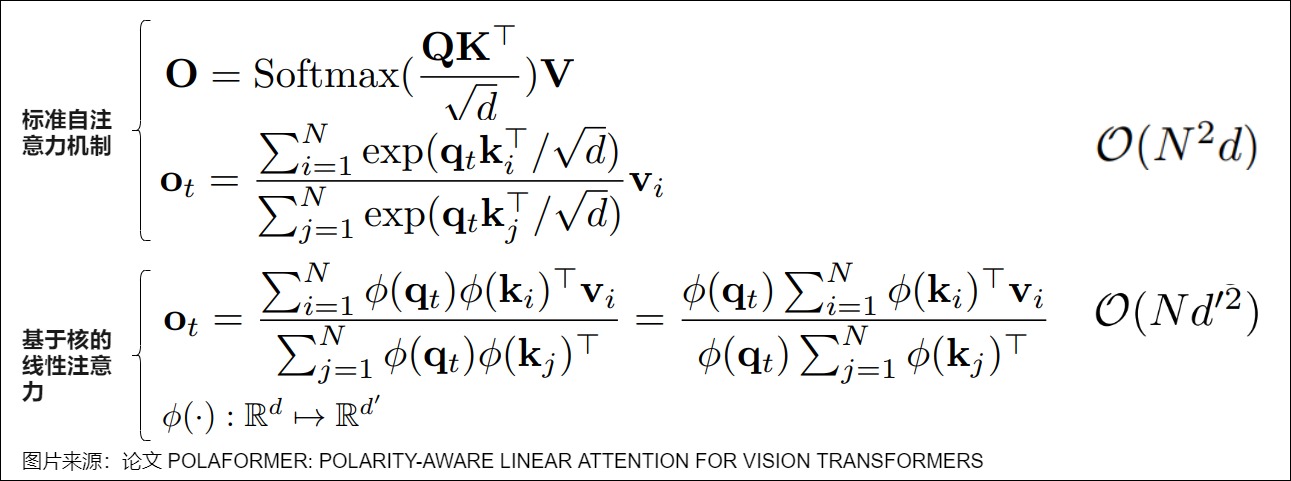
The A10 figure is a useful algebraic map, but its O(N d'^2) label assumes a
particular relation between feature and value widths. It is not a measured
runtime claim.
Linear Transformer chooses a deterministic positive map such as and therefore defines a different kernel from softmax attention. Performer instead uses FAVOR+ positive orthogonal random features to approximate the softmax kernel. These alternatives must not be collapsed:
deterministic kernel replacement:
    exact for the chosen feature kernel
    not exact dense softmax

finite random-feature approximation:
    random estimator of a target kernel
    approximation quality depends on feature count and sampled projection

exact IO-aware softmax:
    exact dense softmax relation within numerical tolerance
    no feature approximation
Positivity is not cosmetic. It keeps similarity and the denominator compatible with normalized weighted averaging. Even then, a tiny denominator, growing summary magnitude, finite-precision drift, and feature-map overflow remain numerical contracts.
Causal kernel attention is a recurrent state and a parallel-prefix problem
For causal rows, update summaries before querying position t:
The state has m*dv + m values per head instead of one stored K/V row per
token. Loop 9 compares the recurrent update with explicit causal pairwise
kernel attention and obtains 5.56e-17 maximum absolute error.
state_kv = zeros(feature_width, value_width)
state_k = zeros(feature_width)

for t in range(sequence_length):
    kt = phi(key[t])
    qt = phi(query[t])
    state_kv += outer(kt, value[t])
    state_k += kt
    output[t] = (qt @ state_kv) / (qt @ state_k)
This recurrence describes one-token execution, not the only training schedule. The prefix operation is associative, so training can use a scan or chunkwise scheme that materializes different intermediates. Saved states, recomputation, chunk boundaries, and backward reductions must be specified separately.
Retention shows that recurrent and parallel forms can share one contract
RetNet removes row softmax and introduces distance decay. In a simplified real form, let:
Unrolling the recurrence gives:
and therefore:
The parallel score form is a causal bilinear interaction multiplied by a decay
matrix. The recurrent state and parallel matrix implement the same simplified
operator; they are not the same as normalized softmax attention. Loop 9’s
gamma=0.8 fixture reconciles the two forms to 4.44e-16 maximum absolute
error.
The RetNet paper defines parallel, recurrent, and chunkwise recurrent representations and adds multi-scale decay, gating, position treatment, and normalization. The equations above isolate only the core equivalence. A full RetNet implementation cannot be reconstructed from this simplified state.
Length projection is an adjacent branch, not kernel attention
Linformer reduces the source-length axis with learned projections. Conceptually:
The probability matrix is now [S,k], but each projected row can mix many
original source rows. This is not a sparse subset of original edges and not a
feature-map reassociation. In a causal decoder, a learned length projection
must prove that projected source rows do not mix future information. That
sequence-axis ownership is why low-rank projection remains a short adjacent
branch here rather than being folded into the kernel state derivation.
Hybrid interaction graphs must be composed in layer order
Hybrids appear at two levels:
within one layer:
    local + random + global routes
    several head-specific graph families

across layers:
    local or recurrent early layers
    linear layers for most of the stack
    periodic full-softmax layers
The layer order is semantic configuration. A full-attention layer gives every row direct access to its legal inputs at that layer. It does not retroactively give earlier sparse layers access to information that had not yet crossed their graph, and information created after the full layer waits until another global route appears.
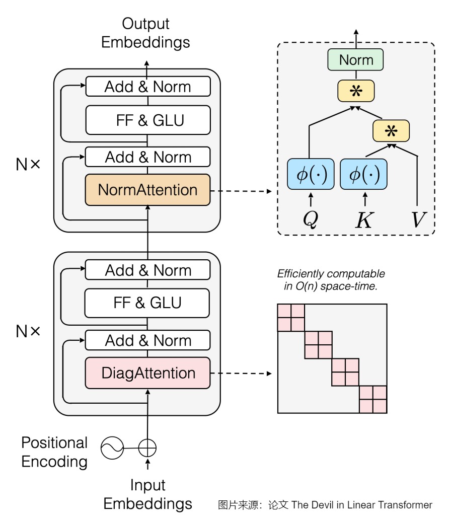
TransNormer uses diagonal/local attention in early layers to address attention
dilution and normalized linear attention later for global mixing. MiniMax-01 is
a different hybrid: its report places one softmax-attention layer after every
seven Lightning Attention layers. That 7:1 schedule is source-reported,
not a universal optimum.
For L_lin linear layers and L_full dense causal layers, a symbolic leading
ledger is:
where the factor 2 counts one feature-state update and one query-state read
per linear layer, before feature construction, denominator work, projections,
normalization, and runtime effects.
If L_full>0 is fixed, the architecture still contains a quadratic term in
S, even when the coefficient is much smaller than an all-softmax stack. The
fixture’s eight-layer 7+1 schedule has one-eighth full layers and 8,256 causal
pairs in its single full layer at S=128.
Paper-by-contract comparison
The purpose of this table is not to rank papers. It identifies the object each paper changes and the state an implementation must preserve.
| Method | Direct interaction contract | Normalization or approximation | Reproducible state | Leading sequence claim | Status |
|---|---|---|---|---|---|
| dense softmax | every legal pair | exact row softmax | Q/K/V, mask, bias, dropout | pair work | M3.1 reference |
| Sparse Transformer | fixed factorized patterns | exact softmax on selected positions | factorization by layer/head | primary-paper verified | |
| Longformer | sliding window plus task global rows; optional dilation | exact softmax on selected positions | window, dilation, global-row policy | linear for fixed route counts | primary-paper verified |
| BigBird | local, random, and global sparse graph | exact softmax on constructed graph | random graph/seed, windows, globals | linear for fixed route counts | primary-paper verified |
| Routing Transformer | online-k-means content routes plus local heads/layers | exact softmax within gathered candidates | centroids, assignment, balance, causal filter | in paper design | primary-paper verified |
| Reformer | LSH-selected candidates | softmax over hashed buckets/rounds | hash projections, rounds, sorting, duplicate policy | reported | primary-paper boundary |
| Linear Transformer | implicit all-source feature summaries | deterministic positive kernel, not softmax | feature map and recurrent summaries | linear in S for fixed widths | primary-paper verified |
| Performer | implicit random-feature summaries | FAVOR+ approximation to softmax kernel | random projection/seed and feature count | linear space/time for fixed features | primary-paper verified |
| RetNet | decay-weighted bilinear history | no row softmax; parallel/recurrent/chunkwise forms | decay, complex/position state, normalization, recurrent state | linear sequence work; recurrent decode | primary-paper verified |
| TransNormer | early diagonal/local plus later normalized linear attention | mixed local and linear operators | layer schedule, normalization, feature map | paper-specific linear design | primary-paper verified |
| MiniMax-01 | seven Lightning layers then one softmax layer | hybrid linear and softmax operators | exact layer schedule and each operator state | retains a reduced quadratic component | source-reported primary report |
| Linformer | learned projection from S rows to k landmarks | softmax over projected rows | length projections and causal policy | linear in S for fixed k | adjacent primary-paper branch |
The asymptotic column is conditional. Window, route, feature, landmark, head,
and value widths can scale; graph construction and projection work can be
nontrivial; and no O(S) label proves a lower wall-clock time at a particular
shape.
Training and runtime integration are part of the architecture
An alternative interaction graph changes more than a forward equation:
| Contract surface | Sparse graph | Kernel/recurrent | Hybrid |
|---|---|---|---|
| training manifest | route pattern/seed, per-head assignment, padding to buckets/blocks | feature map, projection seed, scan/chunk schedule, state dtype | exact layer operator sequence |
| backward | gradients only along selected edges; learned discrete routes need an estimator/update rule | gradients through prefix summaries; saved versus recomputed state | operator-specific backward by layer |
| checkpoint | routing state and topology version | feature projection, decay, normalization, state schema | layer schedule plus every component config |
| prefill | build sparse metadata or parallel summaries | scan/chunk state construction | execute mixed operators in order |
| one-token decode | gather legal sparse history or window cache | update fixed-size recurrent state | some layers append K/V, others update summaries |
| batching | route and block shapes can diverge by request | state shapes may be fixed but numerical age differs | request state is heterogeneous by layer |
M3.10 owns the one-request logical state transition. M5.1 owns the persistent request/cache lifecycle, M5.2 owns multi-request scheduling, and M5.3 owns physical allocation. Loop 9 only states which per-layer state those owners would have to carry.
The M3-to-M4 firewall: semantics, logical work, and physical evidence

M3.1 may derive logical pair counts because they follow from the model graph. It must not infer physical bytes or speed from them:
M3.1 freezes:
    legal edge relation and causal direction
    normalization/value-mixing function
    stacked reachability
    logical edge or summary-state dimensions
    required training and inference state

M4.1 integrates:
    whole-layer/model parameters, FLOPs, activations, and logical traffic

M4.3 proves for exact softmax:
    online state algebra
    tiled forward/backward schedule
    HBM/SRAM transfer bounds
    materialization and recomputation

M4.5 owns:
    decode-specific split work
    mask-program lowering
    backend admission and runtime evidence
Two opposite errors follow from crossing this firewall:
N_edge < S^2, therefore the model must run faster. This ignores block cover density, route construction, sorting/gathers, padding, launch count, occupancy, and fallback.- FlashAttention avoids an
S x SHBM tensor, therefore it is sparse or linear attention. This confuses a physical exact schedule with a changed semantic graph or kernel.
The only publishable performance claim has an evidence coordinate:
model graph + operator parameters
    -> backend lowering and admitted schedule
    -> hardware, dtype, shape, phase, batch state
    -> measured latency/throughput/bytes
M4.1 integrates the local graph ledger into whole-layer and whole-model accounting. M4.3 owns the exact tiled-softmax schedule and IO derivation. M4.5 owns decode-phase backend admission, lowering, and measured dispatch evidence.
How this was checked A table of mistakes made when describing efficient-attention methods, and the conditions the article's test code checks for this section. (about 290 words, 2 code listings)
Loop 9 failure lab
| Failure | Shape still looks valid because | Broken contract | Detection |
|---|---|---|---|
| call local attention “exact dense attention” | every row still normalizes to one | legal edge set changed | compare visible and edge count |
| infer reachability from edge count | two graphs can have equal counts | path composition differs | shortest-path/stacked-relation oracle |
| claim a global token transfers information in one layer | all global edges appear in one mask | synchronous layer reads pre-update states | two-layer influence trace |
| use independent chunks as sliding windows | both expose about Sb cells | chunks disconnect boundaries | cross-chunk reachability test |
| equate semantic edges with block work | block tensor shapes are valid | boundary tiles contain masked slots | report N_edge, N_slot, and rho_B |
| resample random routes without recording a seed | output shape is unchanged | graph identity changes | route manifest hash |
| forget causal filtering after content routing | candidates have plausible similarity | future keys leak | absolute-coordinate legality assertion |
| call deterministic linear attention a softmax approximation | both return [S,dv] | chosen kernel differs | record feature-map contract |
| omit kernel denominator | output shape and leading complexity remain | normalized weighted average is lost | pairwise/reassociated oracle |
| initialize recurrent state after reading the query | state dimensions still match | off-by-one causal semantics | explicit prefix fixture |
| claim constant-memory training from constant-memory decode | recurrent step uses fixed state | backward needs saved or recomputed prefixes | training-state ledger |
| call a 7:1 hybrid linear in all terms | most layers are linear | one full layer retains S^2 work | symbolic layer-sum ledger |
| transfer BigBird theory to any sparse mask | mask is sparse and connected in a sample | theorem assumptions changed | paper-by-contract manifest |
| infer speed from asymptotic notation | arithmetic count is lower | physical schedule may be inefficient | M4 profiler/traffic evidence |
Loop 9 executable gate
The deterministic evidence package freezes the graph and state distinctions:
cd docs/numinens-evidence/m3-1-attention-score-path
python3 loop9_interaction_graph_oracle.py
python3 loop9_contract_audit.py
python3 -m unittest -v test_loop9_contract
Publication requires:
dense and local exact edge-count formulas match enumerated graphs;
local path depth and chunk disconnection are machine checked;
symmetric global routing takes two stacked layers;
semantic edges and block candidate slots remain separate;
pairwise and reassociated kernel attention agree for one feature map;
causal pairwise kernel attention and recurrent summaries agree;
parallel and recurrent retention agree for the simplified contract;
hybrid layer counts expose their remaining quadratic term;
every paper claim is source-qualified;
M4 receives schedules and physical evidence, not model semantics;
Loops 1-8 section hashes remain frozen.
0x0B What M3.1 does not own
| Boundary | M3.1 imports | M3.1 does not re-teach |
|---|---|---|
| M3.3 | optional finite position_bias slot | T5, Shaw, ALiBi, DeBERTa, TUPE |
| M3.4 | Q/K may already have been rotated before scoring | RoPE proof, rotate_half, cache-position geometry |
| M3.5 | long q_len / k_len may stress the score path | PI, NTK, YaRN, LongRoPE |
| M3.9 | masks arrive at the model boundary | target shift, tgt_y, loss masks, label smoothing |
| M3.10 | decode may have q_len=1 and k_len=past+1 | loop, logical append, EOS, active rows, and request-local cache-frontier requirements; persistent cache lifecycle belongs to M5.1 and physical allocation/mutation to M5.3 |
| M3.2 | Q/K/V are already shaped | projection matrices, head split, concat, output projection |
| M4.1 | local MAC and element counts from this article | integrated layer/model totals, training state, HBM traffic, arithmetic intensity |
M3.1 is deliberately narrow because the score path is already enough to debug many real failures.
0x0C Shape ledger
| Object | Shape | Notes |
|---|---|---|
query | [B,h,q_len,d_head] | query rows asking for information |
key | [B,h,k_len,d_head] | matched rows |
value | [B,h,k_len,d_value] | payload rows |
key.transpose(-2,-1) | [B,h,d_head,k_len] | transpose only the last two axes |
scores | [B,h,q_len,k_len] | one logit per query-key pair |
position_bias | [1,h,q_len,k_len] or broadcast-compatible | finite preference, optional |
| source padding mask | [B,1,1,k_len] | hides key/value columns |
| causal mask | [1,1,q_len,k_len] or compatible | hides future keys |
| combined target mask | [B,1,q_len,k_len] or compatible | padding + causal visibility |
masked_scores | [B,h,q_len,k_len] | after finite bias and visibility mask |
| softmax accumulation | [B,h,q_len,k_len] | dtype is an eager/fused backend contract |
p_attn | [B,h,q_len,k_len] | softmax over k_len |
dropout mask on p_attn | [B,h,q_len,k_len] | training-time probability dropout |
out = p_attn @ value | [B,h,q_len,d_value] | per-head contextual output |
| M3.2 merged output | [B,q_len,d_model] | after head concat and output projection |
| M4.1 score/probability object | [B,H_q,S_q,S_k] | cost-model handoff |
Three common mode ledgers:
| Mode | q_len | k_len | Score shape |
|---|---|---|---|
| encoder self-attention | S | S | [B,h,S,S] |
| decoder prefix/training self-attention | T | T | [B,h,T,T] |
| cross-attention | T | S | [B,h,T,S] |
| one-token decode boundary | 1 | past + 1 | [B,h,1,past+1] |
0x0CA Executable Oracle, Gradient Parity, and Reconciliation
This section builds one deliberately difficult test call and uses it to compare scalar and vectorized forward passes, hand-derived and numerical gradients, and differently encoded masks, including tests that must fail when the operation changes. Open it when you write tests for an attention implementation.
How this was checked One adversarial test call comparing scalar and vectorized forward passes, hand-derived and finite-difference gradients, blocked sources, mask adapters and deliberate failures, with the tolerances and a wider test matrix. (about 1,830 words, 10 code listings, 28 equations, 1 figure)
Loops 3 through 9 each froze one part of the attention contract: score families, visibility, stable normalization, dropout and backward, the complete eager trace, runtime adapters, and alternative interaction graphs. Independent fixtures are useful while deriving each mechanism, but they can still leave a gap between them. A final implementation can pass seven isolated examples and fail when finite bias, rectangular axes, fixed dropout state, mask polarity, and gradients meet in one call.
Owner question. Can one deterministic attention call reconcile scalar equations, vectorized eager code, manual backward, numerical derivatives, runtime mask adapters, and alternative-graph expectations without treating every numerical difference as either a backend bug or harmless noise?
Loop 10 adds that reconciliation layer. It does not claim that NumPy predicts the exact reduction order of a GPU kernel. It freezes the semantic baseline, the differentiable variables, the stochastic realization, and the expected verdict for each comparison before a production backend runs.
Four verdicts replace one ambiguous allclose
Two outputs with the same shape do not automatically belong in a parity test. The comparison first declares its relation:
| Verdict | Compared paths | Required evidence | A difference means |
|---|---|---|---|
| exact/float64 parity | scalar loops and vectorized eager evaluation of the same graph | tiny absolute error | implementation defect or oracle defect |
| tolerance parity | same semantic operator under different reduction/derivative evaluation | predeclared atol, rtol, dtype, backend | investigate beyond tolerance |
| invariant | one operator under a symmetry or limiting transformation | property-specific equality | equation or metadata contract was violated |
| expected divergence | polarity, causal alignment, or legal interaction graph changed | output delta above a minimum witness | the test successfully distinguished operators |

This prevents two opposite mistakes:
wrong:
    changed graph produces another output
    -> optimized path is numerically inaccurate

also wrong:
    same graph produces another output
    -> backend differences are always expected

correct:
    declare semantic identity first
    -> choose exact, tolerance, invariant, or divergence gate
    -> record the observed result
The immutable reconciliation fixture is intentionally adversarial
The fixture is one local head, not a full projection stack:
Q:          [2,3]
K:          [5,3]
V:          [5,2]
visible:    [2,5]
finite_bias:[2,5]
keep_mask:  [2,5]
upstream G: [2,2]
output O:   [2,2]
It has five properties that a square random fixture usually misses:
q_len=2andk_len=5, so query and source axes cannot be conflated.- Each query has a different legal set, so visibility is genuinely row-wise.
- Finite bias contains large values on illegal edges; masking must dominate preference without allowing those values back into the denominator.
- Source row four is globally blocked but has value
[1000,-1000]; even a small leak becomes visible. - Dropout probability is
0.25, but the boolean keep matrix is frozen. Every compared differentiable path therefore uses the same realized multiplier:
on legal edges and zero elsewhere.
Freezing the keep matrix is not an inference-time convention. It is a test contract. Resampling dropout between a plus/minus finite-difference evaluation would estimate stochastic noise instead of a derivative of one function.
Scalar and vectorized forwards meet at every named object
For this fixture, the vector path computes:
The scalar path independently loops over query rows and legal source indices:
for i in range(q_len):
    legal = [j for j in range(k_len) if visible[i, j]]
    logits = [scale * dot(Q[i], K[j]) + bias[i, j] for j in legal]
    numerators = exp(logits - max(logits))
    denominator = sum(numerators)
    for j, numerator in zip(legal, numerators):
        P[i, j] = numerator / denominator
        O[i] += P[i, j] * multiplier[i, j] * V[j]
It does not call the vector softmax helper. That independence matters: two wrappers around the same faulty helper are not two oracles.
The generated report obtains:
max |P_scalar - P_vector| = 2.78e-17
max |O_scalar - O_vector| = 5.55e-17
Those are float64 arithmetic differences, not a universal tolerance for fp16/bf16 kernels.
Backward parity starts from one scalar objective
Let the test loss be the Frobenius inner product with an explicit upstream
matrix G:
This is more general than hard-coding O.square().mean(): G makes the
vector-Jacobian product explicit and keeps the derivative trace small.
Because O=CV, the value and consumed-probability gradients are:
The frozen dropout multiplier is elementwise:
For one row, softmax has Jacobian
Multiplying that Jacobian by the incoming row gradient gives the implementation form used by Loop 6 and the reconciliation oracle:
Visibility is applied again to the gradient, not assumed from approximate underflow:
Finally:
The finite-bias derivative is worth retaining. Bias can be broadcast or parameterized by another module; the local score-shaped gradient must be reduced back over exactly those broadcast axes by its owner.
Central differences test the implemented vector-Jacobian product
For each scalar coordinate x_r of Q, K, V, and finite bias, the dependency-
free oracle evaluates:
Central difference has truncation and floating-point error. It is therefore a tolerance test, not a bitwise oracle. The fixture uses float64, avoids softmax ties and visibility changes, and keeps the dropout realization fixed. Those conditions matter because finite differences do not define a useful gradient through a discrete top-k route, a changed boolean mask, a resampled dropout draw, or a branch boundary.
The measured maximum absolute errors are:
| Variable | Manual versus central difference |
|---|---|
| Q | 6.21e-11 |
| K | 1.10e-10 |
| V | 7.42e-11 |
| finite bias | 7.28e-11 |
The gate is fixed at 2e-9, before observing a production backend. PyTorch’s
gradcheck mechanics
similarly compare analytical and numerical derivatives, while warning that the
checking contract depends on function, precision, and numerical assumptions.
For an actual PyTorch implementation, torch.autograd.gradcheck complements
this repository oracle; it does not replace the semantic mask and runtime
tests.
Blocked sources need output and gradient witnesses
An illegal probability being printed as 0.0 is useful but incomplete. Loop
10 perturbs the globally blocked value by [10^6,-10^6] and checks:
output delta after blocked-value perturbation = 0
blocked key-gradient max absolute value       = 0
blocked value-gradient max absolute value     = 0
blocked score/bias gradients                  = 0
This catches four distinct failures:
- a finite sentinel that leaks after a large later bias;
- masking after softmax normalization;
- a backward path that ignores visibility;
- a gather/scatter map that assigns the blocked source another row’s gradient.
For a source blocked only from some queries, its total K/V gradient need not be zero because legal queries can still use it. A zero-gradient assertion must be scoped to an edge or to a globally blocked source, as it is here.
Algebraic invariants do not trust a second implementation
Row-shift invariance. For any row scalar c_i:
Adding [1.75,-2.25] row-wise to finite bias changes Loop 10’s output by only
1.67e-16. A wrong reduction axis generally breaks this property.
Paired source permutation. Let Pi permute source rows. Without an
untransformed order-dependent term:
The fixture transforms K, V, visibility, finite bias, and dropout multiplier
together. Its output delta is 2.78e-17. Permuting K alone is not an invariant;
it changes which value receives each score.
RoPE, relative bias, causal coordinates, packed-example identity, and cache positions are order-dependent state. A permutation test must transform those objects too or explicitly run in a regime where they are absent. M3.3 owns those geometry transformations.
Runtime adapters can differ in representation and still require parity
Loop 8 established opposite boolean conventions:
semantic / functional SDPA boolean:
    True = legal

MultiheadAttention boolean:
    True = blocked
The reconciliation oracle lowers one semantic visibility matrix both ways:
sdpa_visible = visible
mha_blocked = logical_not(visible)
recovered_for_local_oracle = logical_not(mha_blocked)
The two adapted outputs match exactly. Passing the semantic boolean directly
to the blocked-mask API instead produces an output delta above 1000, amplified
by the adversarial illegal value. That is expected divergence proving the
polarity test has power, not an acceptable backend tolerance.
Production SDPA parity needs an environment manifest in addition to semantic inputs:
framework/version
device and compute capability
input and accumulation dtype
requested / eligible / selected / observed backend
determinism settings
training/eval and dropout state
forward and backward tolerances
PyTorch’s version-scoped reproducibility documentation records different determinism characteristics for SDPA backends. Therefore “same output within tolerance” and “bitwise reproducible backward” are different gates.
Expected divergence proves that the oracle distinguishes contracts
A parity suite that only compares equivalent paths can pass even if every fixture is too weak. Loop 10 includes three negative controls:
| Changed contract | Observed max output delta | Correct verdict |
|---|---|---|
| invert boolean polarity | 1000.35 | expected divergence |
| remove legal edges with a narrower interaction graph | 0.244 | expected divergence |
| use upper-left instead of cache-aligned rectangular causality | 0.457 | expected divergence |
The threshold is only 1e-3; the purpose is not to rank the changes by quality.
It proves that the fixture can observe the semantic difference.
By contrast, Loop 9’s pairwise and reassociated programs for the same fixed
positive feature map differ by only 5.56e-17. That is parity. Replacing the
feature map, approximating softmax with finite random features, or changing
the legal edge graph would move the comparison into approximation or expected
divergence.
The reconciliation registry prevents independent loops from drifting
Loop 10 imports each deterministic oracle from Loops 3 through 9, rebuilds its report, canonicalizes JSON keys and separators, and compares it with the frozen expected report. The registry covers:
| Frozen oracle | Replayed contract |
|---|---|
| Loop 3 | score families, scale placement, variance and temperature |
| Loop 4 | causal/padding/packed/cache visibility and all-masked policy |
| Loop 5 | stable softmax, support, temperature, precision edge cases |
| Loop 6 | fixed-dropout forward/backward and recomputation |
| Loop 7 | source-to-tensor scalar/vector/Harvard eager trace |
| Loop 8 | polarity, rectangular causality, GQA, dropout mode, dispatch |
| Loop 9 | graph reachability, block cover, kernel recurrence, retention |
All seven observed canonical hashes equal their frozen hashes. This does not prove the articles are universally correct. It proves that Loop 10 has not quietly redefined an earlier executable contract while composing them.
Tolerances are inputs to the experiment
A production comparison should use:
But choosing atol and rtol after seeing a failure turns the gate into a
description of the current error. Record them with the environment manifest,
then investigate failures by stage:
- verify shape, coordinates, legal support, bias, scale, and dropout draw;
- compare eager intermediate scores/probabilities when available;
- force a math backend before comparing fused backends;
- separate forward from Q/K/V/bias gradient errors;
- repeat determinism checks separately from closeness checks;
- widen tolerance only with a numerical argument and a documented risk.
The test matrix still needs more than this one fixture:
| Case | Required variation | Bug class |
|---|---|---|
| bidirectional self-attention | square plus key padding | padding polarity and broadcast |
| causal training | square lower-triangular support | future leakage |
| rectangular cross-attention | independent query/source lengths | square-axis assumptions |
| cached single query | absolute query position and long source | local-index causality |
| cached query chunk | q_len>1, k_len>q_len | upper-left/lower-right confusion |
| packed examples | block-diagonal causal support | cross-example leakage |
| GQA/MQA | H_q != H_kv | head map and grouped broadcast |
| train/eval | nonzero configured dropout | functional dropout left active |
| fp32/fp16/bf16 | backend-qualified tolerance | overflow, promotion, reduction order |
| gradients | Q/K/V/bias and blocked edges | wrong saved tensor or backward map |
M3.1 owns this semantic matrix. M4.3 owns the fused schedule and IO proof; M4.5 owns backend admission and observed execution; M3.9 owns packed batch construction; M3.10 owns request-local logical cache coordination; M5.1 owns persistent publication/lifecycle, and M5.3 owns physical cache mutation. Their tests should consume the same manifest fields rather than inventing new mask or coordinate conventions.
Loop 10 executable gate
The dependency-light evidence lives beside the article:
cd docs/numinens-evidence/m3-1-attention-score-path
python3 loop10_reconciliation_oracle.py
python3 loop10_contract_audit.py
python3 -m unittest -v \
  test_loop1_contract test_loop2_contract test_loop3_contract \
  test_loop4_contract test_loop5_contract test_loop6_contract \
  test_loop7_contract test_loop8_contract test_loop9_contract \
  test_loop10_contract
The gate requires:
scalar/vector forward errors below the frozen float64 threshold;
Q/K/V/bias manual gradients within the frozen finite-difference threshold;
illegal probabilities and blocked-source gradients exactly zero;
row-shift, paired-permutation, and SDPA/MHA-adapter invariants preserved;
negative controls visibly divergent;
Loops 3-9 reports equal their frozen canonical reports;
Loops 1-9 article-section hashes unchanged.
0x0D Failure lab
This section lists how attention implementations go wrong, from malformed inputs that should be rejected before softmax to errors that keep every shape correct (wrong scale, inverted mask polarity, softmax over the wrong axis), each with a test that exposes it. Its last part records how the article’s sources, figures and links were verified. Open it when you are debugging.
How this was checked Why the failures below are sorted by the stage at which each one can be detected. (about 100 words)
Loop 11: Complete Sources, Visual Provenance, and Link Closure
The final local question is not merely what can go wrong? It is:
At which boundary can each failure be rejected, and what evidence distinguishes a malformed call from a same-shape semantic error?
An attention implementation can satisfy every Python shape operation and still compute the wrong interaction graph, the wrong probability distribution, or the wrong runtime mode. Conversely, a fused backend can differ numerically from the eager reference while remaining semantically valid. A useful failure lab therefore needs more than a list of symptoms. It needs a detection stage, a witness, and an owner.
Edge cases and failure behaviour Thirty-two numbered failures, from malformed calls that must be rejected before softmax to shape-preserving errors (wrong scale, inverted polarity, wrong axis, dropout left on in evaluation), each with its evidence, and an order for triage. (about 1,240 words, 3 code listings)
Five detection stages prevent one vague attention failed verdict
| Stage | What it can prove | Representative evidence | What it cannot prove alone |
|---|---|---|---|
| manifest validation | ranks, named axes, source counts, head divisibility, dtype/device compatibility, mode state | immutable call object plus rejection code | that same-shaped axes carry the intended meaning |
| support validation | every consumed query has legal sources and boolean/additive encodings agree | legal-source counts, blocked-mass assertions | that the chosen legal graph is the intended graph |
| numerical oracle | stable normalization, finite output, gradient parity, blocked-route zeroes | scalar reference, finite differences, invariants | that a production backend actually executed |
| semantic negative control | wrong polarity, wrong scale, unpaired permutations, or changed graphs diverge when they should | non-zero witness against the frozen fixture | performance or kernel identity |
| runtime evidence | requested/eligible/selected/observed backend, train/eval dropout state, fallback reason | profiler and runtime record | architectural intent that was never placed in the call manifest |
The order matters. Reject impossible objects before allocating a large score tensor. Then test support. Then compare numbers. Only after the semantic contract is stable should a runtime claim be attached.
Construction-time rejections: malformed objects must not reach softmax
The following cases are deterministic manifest failures. No tolerance and no backend benchmark is needed.
| ID | Failure | Required rejection |
|---|---|---|
| M3A-F001 | Wrong transpose or incompatible query/key width. query @ key cannot form the intended query-key matrix, or a coincidental rank-four result assigns the wrong meaning to its axes. | require the contracted feature axis of Q and K to equal d_head, and require score shape [B,H_q,q_len,k_len] |
| M3A-F002 | Assuming scores are square. Cross-attention and decode normally have q_len != k_len. | validate query and source axes independently; never infer one from the other |
| M3A-F003 | Visibility or finite-bias shape drift. Broadcastability can hide a missing batch, head, query, or source dimension. | validate the declared broadcast class and the resulting logical score shape |
| M3A-F004 | All keys masked for a consumed query row. Stable softmax has a zero denominator and no probability distribution to return. | reject or route through an explicit unused-row policy before normalization |
| M3A-F005 | Bias or mask contains a non-finite value on a visible edge. NaN and unintended +inf contaminate the row. | require finite visible logits; reserve -inf only for physically encoded exclusion |
| M3A-F006 | Bias, mask, and scores live on incompatible devices or use an unapproved dtype conversion. | resolve device and accumulation-dtype policy before score construction |
| M3A-F007 | Value length differs from key length. p_attn has a k_len axis, so V needs the same source-row count as K. | require K.shape[-2] == V.shape[-2] |
| M3A-F008 | GQA replication is not integral. The local mapping requires H_q % H_kv == 0. | reject before any repeat/interleave operation |
A compact validator should fail closed:
def validate_attention_manifest(call):
    require_rank(call.Q, 4)
    require_rank(call.K, 4)
    require_rank(call.V, 4)

    B, H_q, q_len, d_head = call.Q.shape
    B_k, H_kv, k_len, d_key = call.K.shape
    B_v, H_v, v_len, d_value = call.V.shape

    require(B == B_k == B_v, "BATCH_MISMATCH")
    require(d_head == d_key, "QUERY_KEY_WIDTH_MISMATCH")
    require(H_kv == H_v and k_len == v_len, "KEY_VALUE_SOURCE_MISMATCH")
    require(H_q % H_kv == 0, "INVALID_GQA_HEAD_DIVISIBILITY")

    score_shape = (B, H_q, q_len, k_len)
    require_broadcast_class(call.visible, score_shape, "VISIBILITY_SHAPE_MISMATCH")
    require_broadcast_class(call.finite_bias, score_shape, "BIAS_SHAPE_MISMATCH")
    require_every_used_row_has_source(call.visible, "ALL_MASKED_USED_ROW")
    require_finite_on_visible_edges(call.finite_bias, call.visible,
                                    "NONFINITE_VISIBLE_BIAS")
    require_mode_dropout(call.mode, call.dropout_p,
                         "FUNCTIONAL_DROPOUT_ACTIVE_IN_EVAL")
This validator does not prove that True means visible, that the causal coordinates
are correct, or that the scale uses d_head. Those are same-shape semantic properties.
Same-shape semantic failures need discriminating witnesses
| ID | Failure | Why shape checks pass | Witness |
|---|---|---|---|
| M3A-F009 | Using d_model instead of d_head. | both are scalar divisors | compare against the frozen d_head^{-1/2} oracle; probability and output differences must exceed the negative-control threshold |
| M3A-F010 | Missing the scale. | score shape is unchanged | increasing d_head changes logit variance and softmax saturation; Loop 3 freezes the intended temperature |
| M3A-F011 | Mask applied after softmax. | both operations return score-shaped arrays | legal rows no longer sum to one because blocked logits influenced the denominator |
| M3A-F012 | Mask polarity inverted. | visible and blocked tensors have identical shape and dtype | the Loop 10 adversarial fixture produces a large output divergence |
| M3A-F013 | Finite bias used as a mask. | a large negative finite number is a valid floating-point score | blocked mass is small but non-zero; preference is not structural illegality |
| M3A-F014 | Bias added after finite masking. | every operation is broadcast-valid | a sufficiently positive later bias can revive an illegal edge |
| M3A-F015 | Padding mask hides query rows instead of key columns. | square fixtures can conceal the axis swap | perturb a PAD value row; legal output must remain invariant when that source column is blocked |
| M3A-F016 | Causal triangle reversed or cache coordinates anchored incorrectly. | upper- and lower-triangular masks have the same shape | compare absolute-position legality on a rectangular cached-decode fixture |
| M3A-F017 | Softmax over the query axis. | dim=-2 returns the same tensor shape | key-axis row sums differ from one and query rows no longer choose source keys |
| M3A-F018 | Source permutation is not applied jointly to K, V, support, bias, and dropout realization. | every independently permuted tensor still has a legal shape | a paired permutation is invariant; an unpaired key permutation must diverge |
| M3A-F019 | Source padding support is reused as target causality. | equal source and target lengths can make masks shape-compatible | cross-attention source columns must not inherit future-target semantics |
| M3A-F020 | A changed interaction graph is treated as backend parity. | dense and sparse methods can share output shape | classify it as expected divergence, not a failed exact-backend comparison |
The crucial testing rule is:
same shape + same dtype + finite output
    does not imply
same attention semantics
A negative control is useful only when it would fail under the defect it is meant to detect. The wrong-polarity, wrong-scale, unpaired-permutation, and rectangular-causal fixtures are therefore frozen alongside the positive reference.
Softmax, dropout, and value-mixing failures cross phase boundaries
-
Dropout applied to scores or values instead of probabilities. This is a different estimator, not an implementation detail. The Harvard source and the Transformer contract apply dropout to
p_attnbefore value mixing. -
Functional SDPA dropout left active during evaluation. PyTorch functional SDPA applies the supplied
dropout_p; the caller must pass zero outside training. A module’s.eval()flag does not silently rewrite an arbitrary functional argument. -
Post-dropout attention rows assumed to sum to one in every sample. Inverted dropout preserves each probability link in expectation. A realized row can sum below one, above one, or even to zero.
-
Returned
p_attnmistaken for contextual state. The state output isp_attn @ value; its final axis isd_value, notk_len. -
Output row count mistaken for source row count. Attention emits one contextual vector per query, so output length is
q_len. -
Globally blocked source changes output or receives K/V gradient. Perturbing that value row must not change output, and its key/value gradients must be exactly zero in the frozen float64 fixture.
-
A resampled dropout mask is used for finite differences or backend parity. The compared programs no longer have the same realized stochastic input. Freeze RNG identity or the realized multiplier.
Precision and runtime failures require environment evidence
-
Low-precision softmax assumed backend-independent. Eager and fused paths may use different reduction trees and accumulation policies. Use dtype- and backend-specific tolerances after semantic invariants pass.
-
A requested kernel is reported as the observed kernel. Request, eligibility, selection, and observation are separate facts. A fallback is not evidence that the preferred backend ran.
-
Requesting weights silently changes the execution path. Some module paths materialize weights or leave an optimized route when
need_weights=True. The returned API object is part of the runtime contract. -
Decode score is modeled as
[S,S]. One-token decode normally scores[B,H_q,1,past+1]. M3.10 owns the request-local logical cache frontier; M5.1 owns persistent publication and M5.3 physical mutation; M3.1 owns the local call coordinates. -
Materialized score assumptions leak into semantics. Fused exact attention can preserve the logical score path without storing the full pair matrix in HBM. M4.3 owns that schedule and IO proof.
Failure triage follows the first violated invariant
1. freeze the call manifest and environment
2. reject rank, axis, source-count, head-map, device, and mode mismatches
3. inspect legal-source counts and all-masked rows
4. run scalar/vector forward parity in float64
5. run blocked-mass, row-sum, permutation, and row-shift invariants
6. freeze dropout, then compare backward and finite differences
7. run expected-divergence controls
8. compare runtime adapter outputs under declared tolerances
9. attach profiler evidence only after semantic parity passes
How this was checked How the article's failure fixtures, sources, figures and internal links were verified, and what that verification does not prove. (about 590 words, 2 code listings, 1 figure)
The executable Loop 11 fixture contains both rejection cases and same-shape defects. Each must produce its declared error code or numerical witness. Merely raising some exception does not pass the test.

The publication gate is a chain: an object rejected at an earlier boundary never earns a later numerical or runtime claim.
Complete source closure is an inventory, not a larger bibliography
The article’s references play different evidential roles:
| Class | Allowed use | Forbidden shortcut |
|---|---|---|
| immutable local Transformer articles | source-local explanation, historical organization, and retained author figures | treating source-local prose as independent external verification |
| primary papers | mechanism, derivation, algorithm contract, and source-reported results within the paper’s setup | converting a paper result into a universal runtime guarantee |
| official framework documentation | current API semantics, argument conventions, and documented backend behavior | assuming a moving documentation URL describes every installed version |
| project or author engineering source | implementation orientation and source lineage | using it as sole support for an unrelated theoretical or benchmark claim |
| contextual analysis | interpretation and boundary-setting | presenting interpretation as a paper claim |
Loop 11 extracts every https:// URL from the article, joins it against the frozen Loop
1-10 source manifests plus a supplemental audit for older citations, and requires exact set
equality. An uncatalogued article URL fails. A stale manifest URL not used by the article is
allowed as upstream research history, but it does not count as a published citation. Network
reachability is deliberately a separate dated audit; reproducible offline closure concerns
identity, classification, and claim scope.
The two immutable local source owners remain:
- A10, Transformer Series Self-Attention, for self-attention lineage and retained figures;
- A11, Transformer Series Mask, for mask construction, mask figures, and source-local implementation history.
Their hashes are recorded. Loop 11 does not edit them.
Visual provenance closes every published asset route
The article mixes three legitimate visual classes:
- repository-authored diagrams and executable-fixture reconstructions;
- diagrams reused from another Transformer System owner with an explicit local lineage;
- retained figures from the author’s original Transformer articles.
The visual manifest extracts every Markdown image and every <picture> source/fallback,
checks that each route resolves under public/, hashes the file, parses SVG XML, records its
semantic job from the alt text, and checks responsive pair closure. It does not claim that a
provenance record creates new rights. Source-local inherited figures retain their original
lineage; newly authored diagrams state that no paper artwork was copied.
A visual fails closure when any of these is true:
route unresolved
empty semantic alt text
malformed SVG
mobile source without its desktop fallback
desktop/mobile paths present but only one is published
asset lacks provenance class, semantic job, or reuse decision
Local-link closure checks ownership, not just HTTP syntax
Every /posts/<slug> link is resolved to src/content/posts/<slug>.md. The manifest records
the destination title and the reason for the handoff. That catches an old slug even when a
development server happens to return a generic page.
The boundary is deliberate:
- M3.2 owns head projection, layout, concatenation, and output projection;
- M3.3-M3.5 own positional geometry and context extension;
- M3.9 owns training batch, position, attention, and loss-mask alignment;
- M3.10 owns request-local logical cache coordination, positions/frontiers, and one-request transitions;
- M5.1 owns persistent request/cache schema, publication, and lifecycle;
- M5.2 owns multi-request admission, scheduling, and preemption;
- M5.3 owns physical cache allocation, reference ownership, copy-on-write, and mutation;
- M4.1 owns whole-model arithmetic and memory ledgers;
- M4.3 owns exact tiled schedules and IO complexity;
- M4.5 owns backend eligibility, fallback, profiling, and observed execution.
Loop 11 may verify that those links exist. It may not absorb their mechanisms into M3.1.
Loop 11 executable gate
The frozen closure passes only when all of the following hold:
- every declared invalid fixture is rejected by its expected code or witness
- wrong-axis, wrong-polarity, wrong-scale, and unpaired-permutation controls diverge
- blocked-source and legal permutation invariants still hold
- every external URL is present in the complete source inventory
- A10 and A11 remain hash-identical
- every local post route resolves to a Markdown owner
- every published image route resolves and every SVG parses
- responsive image pairs are complete
- Loops 1-10 section hashes remain unchanged
- the Loop 11 section hash matches the frozen contract
This is publication closure, not production exhaustiveness. It proves that the article’s declared examples, failures, sources, visuals, and handoffs agree with one another. It does not prove every accelerator, framework version, or model integration correct.
0x0E Handoff to M3.2 and M4.1
M3.1 ends with a function that assumes Q/K/V are already available:
out, p_attn = attention(query, key, value, mask=mask, dropout=dropout)
M3.2 opens the caller:
X: [B,S,d_model]
  -> W_Q, W_K, W_V projections
  -> [B,S,d_model]
  -> view [B,S,h,d_head]
  -> transpose [B,h,S,d_head]
  -> attention(...)
  -> transpose / contiguous / view
  -> output projection W_O
So M3.1 owns:
scores -> mask/bias -> softmax -> p_attn -> weighted values
M3.2 owns:
projection -> head layout -> attention call -> concat -> output projection
That split keeps the block stack readable. First understand how one attention call works. Then understand how the Transformer packs many heads around it.
M4.1 receives the same objects as a ledger:
Q:        [B, H_q, S_q, d_h]
K:        [B, H_kv, S_k, d_h]
V:        [B, H_kv, S_k, d_h]
scores:   [B, H_q, S_q, S_k]
p_attn:   [B, H_q, S_q, S_k]
out_head: [B, H_q, S_q, d_h]
M3.1 defines the tensors and derives their local element and arithmetic counts. M4.1 integrates those counts across layers and execution phases, then asks which objects are materialized, how many bytes reach HBM, and whether the schedule is compute- or bandwidth-bound.
0xFF References
- Exploring the Transformer Series (1) — Attention Mechanism
- Exploring the Transformer Series (2) — Overall Architecture
- Exploring the Transformer Series (10) — Self-Attention
- Exploring the Transformer Series (11) — Mask
- Exploring the Transformer Series (12) — Multi-head Self-Attention
- M1.1 — Why Transformers, Which Architecture, and What Executes
- M2.1 — Tokenization and Sequence Contracts
- M2.2 — Embeddings and Initial Model State
- M3.9 — Training Execution
- M3.10 — Single-Request Inference Execution
- M3.3 — Positional Geometry and Attention Bias
- M3.4 — Rotary Position Embedding
- M3.5 — Context Extension
- M3.2 — Multi-Head Attention Layout
- M4.1 — Transformer Cost Model
- M4.3 — IO-Aware Exact Attention
- M4.5 — Decode Kernels and Backend Boundaries
- Vaswani et al., Attention Is All You Need
- Bahdanau et al., Neural Machine Translation by Jointly Learning to Align and Translate
- Luong et al., Effective Approaches to Attention-based Neural Machine Translation
- Britz et al., Massive Exploration of Neural Machine Translation Architectures
- Henry et al., Query-Key Normalization for Transformers
- Ferrando et al., A Primer on the Inner Workings of Transformer-based Language Models
- Blanchard, Higham, and Higham, Accurate Computation of the Log-Sum-Exp and Softmax Functions
- Milakov and Gimelshein, Online normalizer calculation for softmax
- Veličković et al., Softmax is not Enough (for Sharp Size Generalisation)
- Martins and Astudillo, From Softmax to Sparsemax: A Sparse Model of Attention and Multi-Label Classification
- Peters, Niculae, and Martins, Sparse Sequence-to-Sequence Models
- Srivastava et al., Dropout: A Simple Way to Prevent Neural Networks from Overfitting
- Rush, The Annotated Transformer
- Lin et al., DropAttention: A Regularization Method for Fully-Connected Self-Attention Networks
- Li et al., DropKey for Vision Transformer
- Zhou et al., Scheduled DropHead: A Regularization Method for Transformer Models
- Jain and Wallace, Attention is not Explanation
- Wiegreffe and Pinter, Attention is not not Explanation
- Dao et al., FlashAttention: Fast and Memory-Efficient Exact Attention with IO-Awareness
- Child et al., Generating Long Sequences with Sparse Transformers
- Beltagy et al., Longformer: The Long-Document Transformer
- Zaheer et al., Big Bird: Transformers for Longer Sequences
- Roy et al., Efficient Content-Based Sparse Attention with Routing Transformers
- Kitaev et al., Reformer: The Efficient Transformer
- Katharopoulos et al., Transformers are RNNs: Fast Autoregressive Transformers with Linear Attention
- Choromanski et al., Rethinking Attention with Performers
- Sun et al., Retentive Network: A Successor to Transformer for Large Language Models
- Qin et al., The Devil in Linear Transformer
- MiniMax et al., MiniMax-01: Scaling Foundation Models with Lightning Attention
- Wang et al., Linformer: Self-Attention with Linear Complexity
- Krell et al., Efficient Sequence Packing without Cross-contamination
- Bai et al., LongAlign: A Recipe for Long Context Alignment of Large Language Models
- Kundu et al., Enhancing Training Efficiency Using Packing with Flash Attention
- PyTorch 2.13 documentation,
torch.nn.functional.scaled_dot_product_attention - PyTorch documentation,
torch.nn.functional.softmax - PyTorch documentation,
torch.nn.functional.dropout - PyTorch documentation,
torch.matmul - PyTorch documentation, broadcasting semantics
- PyTorch documentation,
torch.softmax - PyTorch documentation,
torch.logsumexp - PyTorch 2.13 documentation,
torch.nn.attention.bias.CausalBias - PyTorch 2.13 documentation,
torch.nn.attention.sdpa_kernel - PyTorch 2.13 documentation,
torch.nn.MultiheadAttention - PyTorch 2.13 documentation, reproducibility and CUDA scaled-dot-product attention
- PyTorch tutorial, Implementing High-Performance Transformers with Scaled Dot Product Attention
- PyTorch, FlexAttention: The Flexibility of PyTorch with the Performance of FlashAttention
- PyTorch, FlexAttention Part II: FlexAttention for Inference
- Hugging Face Transformers
v5.13.1,eager_attention_forward - Hugging Face Transformers
v5.13.0, Attention backends andAttentionMaskInterface