X1.1 - Unitization and Geometry Metadata Across Modalities

0x00 The representation problem comes before the encoder

A multimodal system is often introduced as a model that accepts text, images, audio, video, or actions. That description is correct at the product boundary and incomplete at the Transformer boundary. A Transformer layer does not receive a JPEG, a PDF page, a waveform, or a robot trajectory. It receives rows of numerical state and masks over those rows.

The conversion therefore begins before attention and before the modality encoder:

raw object
    -> choose addressable units
        -> preserve unit metadata and validity
            -> encode the units
                -> project or fuse the encoded states

The owner question for this article is:

Which pieces of a non-text object should become individually addressable model state, and which geometry must remain aligned with those pieces?

The answer is not “turn everything into tokens.” Text tokenization is one instance of a broader unitization contract. The contract is the tuple

$$\mathcal{U}(r) = (U, G, V, O),$$

where:

r: raw object
U: ordered or structured units produced from r
G: geometry or structural metadata aligned with U
V: validity mask for real versus padded/missing units
O: origin mapping back to the raw object

The later encoder may replace every unit with a learned vector, but it cannot reliably reconstruct evidence that unitization already cropped, pooled, sampled, merged, misordered, or detached from its metadata.

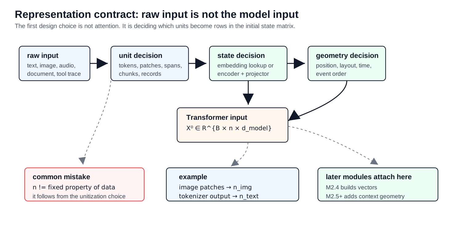
The figure should be read from left to right as an information boundary. The unit sequence decides the future row count. Encoding changes the contents of those rows. Projection changes their width or count. Geometry tells later computation where the rows came from.

What X1.1 owns and defers

X1.1 owns raw-object decomposition, row identity, granularity, geometry metadata, ragged batching, sequence budgets, and the failure modes created before encoding. M2.1 owns text tokenizer algorithms. M2.2 owns the general embedding/projector contract. X1.2 owns modality encoders, projectors, resamplers, and fusion. X1.3 owns multimodal masks, labels, training, runtime state, and serving.

---

0x01 Why one raw object can produce many valid sequences

The initial Transformer state has shape

$$X^0 \in \mathbb{R}^{B \times N \times d_{\text{model}}}.$$

It is tempting to treat $N$ as a property of the input. It is actually an output of preprocessing policy. The same image can become one global vector, 196 fixed patches, thousands of high-resolution patches, OCR spans, detected regions, or a mixture of those units. The same video can become sampled frames, frame patches, tubelets, clips, object tracks, or events.

That choice jointly controls four quantities:

addressability:
    which evidence later attention can select separately

resolution:
    how much local spatial, temporal, or structural detail survives

row count:
    how much encoder, projector, prefill, and cache work follows

inductive bias:
    which relationships are explicit rather than left for the model to infer

Finer units do not automatically produce a better model. They preserve more local evidence while increasing row count and fragmenting context. Coarser units reduce work while forcing multiple facts into one state. A useful unitizer therefore cannot be judged only by output shape. It must be judged by the tasks whose evidence must remain addressable.

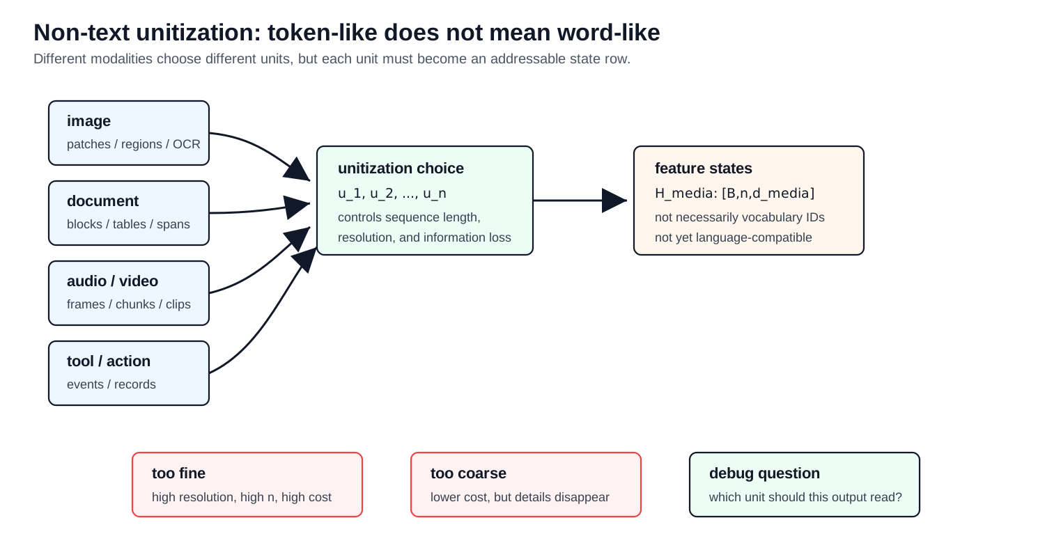
Discrete, continuous, and structured paths

Three implementation paths recur.

discrete path:
    raw object -> token IDs -> embedding lookup

continuous path:
    raw object -> continuous units -> encoder features -> projector

structured path:
    raw object -> typed records + metadata -> field encoders / serializer

These paths can coexist. A document model may use OCR token IDs, image patches, and bounding boxes. A vision-language-action model may use continuous camera features and discrete action tokens. Treating the entire example as one input_ids tensor hides these different contracts.

Unitization is an allocation policy, not a synonym for tokenization

Transformer Series A6 begins from the fact that a model cannot consume an abstract symbol directly: it needs a numerical representation. X1.1 generalizes that observation. Before asking how a unit is embedded, we must decide what earns one row. This is an allocation policy over evidence.

Three tests separate that policy from a convenient file conversion:

coverage:
    can every task-relevant observation be addressed by at least one unit?

separation:
    do facts that must be selected independently occupy distinct units?

stability:
    do training and serving produce the same units, order, geometry, and IDs?

The tests explain why no universal granularity exists. One vector per image is stable and cheap but fails separation for two small objects. One pixel per row has maximal local coverage but produces an unusable sequence and leaves the model to infer useful grouping. Unitization sits between those extremes and introduces an inductive bias: it declares which local changes matter enough to be separately represented.

The unitizer also has two different notions of reversibility:

syntactic reversibility:
    can the stored unit payload be decoded back to the encoded object?

semantic sufficiency:
    can the downstream task still distinguish every case that changes its answer?

Patch extraction can be syntactically reversible when all patches are retained, yet resizing before patch extraction has already removed detail. OCR text can be decoded perfectly while the font, color, and non-text graphics have disappeared. Losslessness must therefore be stated for the complete preprocessing path, not only its final serializer.

A continuous concept can also be one unit

A6 uses Large Concept Models as a counterexample to the assumption that model units must be discrete subwords. The LCM paper defines a proof-of-feasibility concept as a sentence represented in the continuous SONAR embedding space; its model predicts the next sentence-level representation rather than the next vocabulary ID. SONAR supports text and speech inputs, so the unit boundary can be shared across language and modality even though the upstream encoders differ.

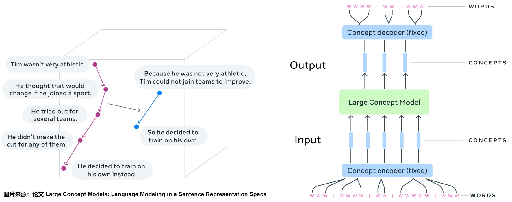
Source reused from Transformer Series A6, based on Large Concept Models. The figure is evidence for a granularity alternative, not a claim that sentence units dominate subword models.

This design changes all four parts of the contract:

Contract part	Subword path	LCM-style concept path
Unit boundary	tokenizer merge rules	sentence segmentation policy
Unit value	discrete vocabulary ID	continuous encoder vector
Generation target	categorical next-token distribution	regression, diffusion, or quantized next-concept objective
Reconstruction	text tokenizer decode	fixed concept decoder back to text or speech

Sentence units shorten the sequence and expose a higher semantic abstraction, but they also hide within-sentence order and make segmentation, encoder version, normalization, and decoder identity part of the checkpoint. This is exactly the X1.1 lesson: changing granularity moves information and compatibility boundaries; it does not make them disappear.

---

0x02 Images: deriving patch rows rather than naming them

Let an image tensor be

$$I \in \mathbb{R}^{B \times C \times H \times W}.$$

For non-overlapping square patches of side $P$, assume $H$ and $W$ are divisible by $P$. There are $H/P$ patch rows and $W/P$ patch columns, so the number of units is

$$N_{\text{patch}} = \frac{H}{P}\frac{W}{P} = \frac{HW}{P^2}.$$

This equation is not merely a notation convention. It explains why halving the patch side multiplies the row count by four: both grid axes double.

The non-overlapping formula is one point in the general sliding-window contract. For kernel size $K$, stride $S$, padding $p$, and dilation $\delta$, one spatial axis of length $H$ produces

$$H_{\text{out}} = \left\lfloor \frac{H+2p-\delta(K-1)-1}{S}+1 \right\rfloor.$$

The same expression gives $W_{\text{out}}$. Therefore $N_{\text{patch}}=H_{\text{out}}W_{\text{out}}$. The ViT setting is recovered with $K=S=P$, $p=0$, and $\delta=1$. Overlapping patches use $S<K$; padded dynamic-resolution models may use $p>0$ or explicit right/bottom padding. The formula must be serialized with the processor because two patchifiers can emit the same row width and different row identities.

Each patch contains $P^2C$ scalar samples. Flattening and applying a learned matrix gives

$$x_{i,j} = \operatorname{vec}(I_{iP:(i+1)P,\,jP:(j+1)P}),$$ $$e_{i,j} = x_{i,j}W_{\text{patch}} + b, \qquad W_{\text{patch}} \in \mathbb{R}^{P^2C \times d_v}.$$

The grid coordinate $(i,j)$ is part of the unit contract even if the tensor is later flattened to sequence index $s=i(W/P)+j$.

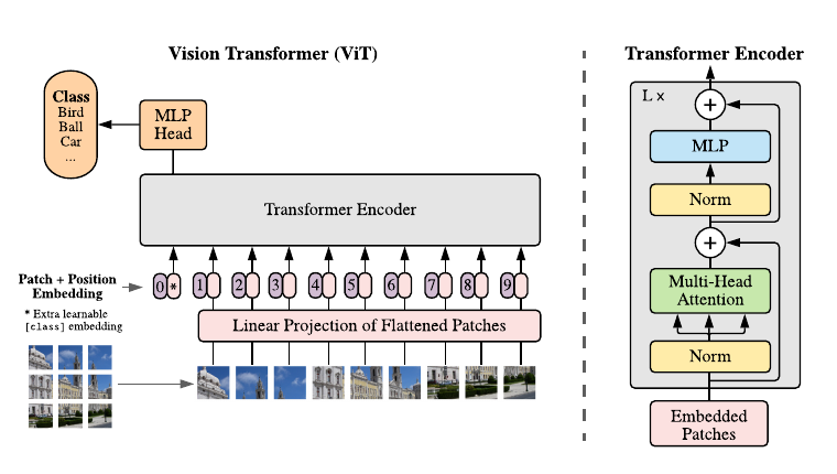
Source: An Image is Worth 16x16 Words, Figure 1. The important X1.1 step is the image-to-patch sequence and its retained grid, not the classifier head.

A tensor-level patch trace

def patchify(images, patch_size):
    # images: [B, C, H, W]
    B, C, H, W = images.shape
    P = patch_size
    assert H % P == 0 and W % P == 0

    gh, gw = H // P, W // P
    patches = images.unfold(2, P, P).unfold(3, P, P)
    # [B, C, gh, gw, P, P]
    patches = patches.permute(0, 2, 3, 1, 4, 5)
    # [B, gh, gw, C, P, P]
    patches = patches.reshape(B, gh * gw, C * P * P)

    row = torch.arange(gh).repeat_interleave(gw)
    col = torch.arange(gw).repeat(gh)
    grid = torch.stack([row, col], dim=-1)  # [N_patch, 2]
    return patches, grid

The permute is part of correctness. If flattening uses a different axis order while grid retains row-major order, the shapes remain valid and every coordinate points to the wrong patch.

Flatten-and-project is exactly a strided convolution

The paper writes patchification as flattening followed by a linear map. A Conv2d with kernel and stride equal to $P$ computes the same operation because each output location takes the inner product between one $C\times P\times P$ receptive field and one learned kernel per output channel:

$$Y_{b,k,i,j} = b_k+ \sum_{c=1}^{C}\sum_{u=0}^{P-1}\sum_{v=0}^{P-1} W_{k,c,u,v}I_{b,c,iP+u,jP+v}.$$

Reshaping $W_{k,:,:,:}$ to one column of $W_{\text{patch}}$ makes this equation identical to $\operatorname{vec}(\text{patch}_{i,j})W_{\text{patch}}+b$. This equivalence matters when checking checkpoints: the parameter may be stored as [d_v, C, P, P] even though the paper describes [P*P*C, d_v].

patch_proj = nn.Conv2d(
    in_channels=C,
    out_channels=d_v,
    kernel_size=P,
    stride=P,
)

grid_states = patch_proj(images)          # [B, d_v, gh, gw]
states = grid_states.flatten(2).transpose(1, 2)  # [B, gh*gw, d_v]

# Row s and grid cell (i, j) must remain inverse mappings.
s = i * gw + j
assert torch.equal(states[:, s], grid_states[:, :, i, j])

This code crosses the X1.1/X1.2 boundary: patch window and row identity belong here; learned projection weights and later encoder states belong to X1.2.

Alternative image units

Unit	What it preserves	What it assumes or risks
Global pooled vector	scene-level summary, low row count	small objects and local text may disappear
Fixed patches	uniform dense coverage	background receives as many rows as evidence-rich areas
Overlapping patches	smoother local continuity	more rows and duplicated pixels
Multi-scale tiles	small evidence plus global view	duplicate content and difficult origin bookkeeping
Detected regions/objects	semantic objects and boxes	detector ontology and recall limit the evidence
OCR spans	textual content and boxes	OCR errors and non-text visual evidence remain
Learned latent queries	fixed row budget	compression can omit rare local evidence

The design choice is therefore not “patches versus no patches.” It is whether the system needs uniform low-level coverage, semantic regions, text spans, multiple scales, or a bounded summary. Many production systems combine them.

Resizing, cropping, tiling, and positional-grid compatibility

For a source pixel coordinate written in homogeneous form $p=(x,y,1)^\top$, a resize, crop, or tile offset is an affine transform

$$p'=Ap, \qquad A= \begin{bmatrix} s_x & 0 & -\Delta_x\\ 0 & s_y & -\Delta_y\\ 0 & 0 & 1 \end{bmatrix}.$$

The patch origin map should retain either this transform or enough fields to reconstruct it. A tile-local cell (i, j) is not globally meaningful without tile_id, scale, crop offset, and source dimensions. When the input resolution changes, a learned ViT position table also changes grid shape. The original ViT fine-tuning recipe interpolates the pretrained 2D position embeddings to the new grid. Interpolation repairs the table shape; it does not restore pixels removed by an earlier resize or make a projector trained on one row policy automatically compatible with another.

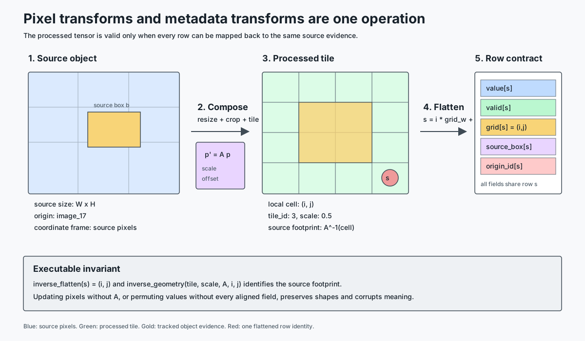
A deployable image processor therefore needs more than image_size:

image_unitizer_manifest = {
    "resize_mode": "shortest_edge",
    "resize_target": 336,
    "crop_mode": "center",
    "crop_size": (336, 336),
    "pad_mode": None,
    "patch_kernel": (14, 14),
    "patch_stride": (14, 14),
    "flatten_order": "row-major",
    "position_grid": (24, 24),
    "pixel_normalization": "checkpoint-specific",
}

Changing any field can preserve tensor rank while invalidating origin maps, position tables, projector binding, cache keys, or all four.

Numeric image budget

336 x 336 image, patch 14:
    24 x 24 = 576 patch rows

1024 x 1024 image, patch 16:
    64 x 64 = 4,096 patch rows

1024 x 1024 image, patch 8:
    128 x 128 = 16,384 patch rows

The last configuration preserves four times the rows of the P=16 case, not twice. This quadratic response to linear resolution is why resizing, tiling, patch merging, and learned resampling are architectural decisions rather than cosmetic preprocessing.

---

0x03 Documents and screenshots: geometry is part of identity

A document is not only an image and not only its OCR text. It may contain:

words and subwords
bounding boxes
page and block identifiers
reading order
table rows and columns
figures and captions
visual patches

For an OCR span $u_i$, a practical record is

$$u_i = (\text{text}_i, b_i, p_i, r_i, c_i, q_i),$$

where $b_i=(x_0,y_0,x_1,y_1)$ is a box, $p_i$ is page, $r_i$ is reading-order index, $c_i$ is an optional structural class, and $q_i$ is confidence. The box must be transformed by the same resize/crop operation as the pixels.

If an original page of size $(W,H)$ is resized to $(W',H')$, the coordinate transform is

$$x' = x\frac{W'}{W}, \qquad y' = y\frac{H'}{H}.$$

If the page is then cropped at offset $(\Delta_x,\Delta_y)$, coordinates become

$$x''=x'-\Delta_x, \qquad y''=y'-\Delta_y.$$

These equations explain a common silent failure: pixel preprocessing changes the image while the boxes retain original coordinates. The arrays still have matching lengths, but their geometry no longer describes the pixels.

Coordinate normalization is a quantized geometry codec

Layout-aware models commonly map pixel coordinates to a bounded integer range. For a target range $[0,R]$, one possible convention is

$$\widehat x= \operatorname{clip}\left( \left\lfloor R\frac{x}{W'}\right\rfloor,0,R \right), \qquad \widehat y= \operatorname{clip}\left( \left\lfloor R\frac{y}{H'}\right\rfloor,0,R \right).$$

LayoutLM-family processors typically use a normalized 0—1000 coordinate space. This is not a cosmetic scale change. Rounding makes the transformation lossy, and the coordinate convention determines valid embedding-table indices. The manifest must state whether boxes are inclusive or half-open, whether normalization occurred before or after cropping, and whether width/height are embedded directly or derived from corners.

OCR introduces another alignment decision because one recognized word can split into several subword IDs. Common policies repeat the word box for every subword or attach geometry only to the first subword and mask the rest for token-level labels. Both are shape-valid. They create different supervision and attention geometry, so the policy must be identical at training and serving.

def normalize_box(box_xyxy, image_hw, bins=1000):
    H, W = image_hw
    x0, y0, x1, y1 = box_xyxy
    q = torch.tensor([
        math.floor(bins * x0 / W),
        math.floor(bins * y0 / H),
        math.floor(bins * x1 / W),
        math.floor(bins * y1 / H),
    ]).clamp_(0, bins)
    assert q[0] <= q[2] and q[1] <= q[3]
    return q

def expand_word_to_subwords(word_id, word_box, tokenizer):
    pieces = tokenizer.encode(word_id.text, add_special_tokens=False)
    return [(piece, word_box, word_id.origin) for piece in pieces]

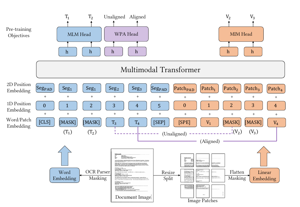
Source: LayoutLMv3, Figure 3. It demonstrates that word identity, 1D order, 2D layout, and image patches are distinct representation objects.

The figure also exposes a training-driven reason to preserve alignment. LayoutLMv3 concatenates text and image-patch embeddings, uses masked language modeling and masked image modeling, and adds a word-patch alignment objective: for a text word, predict whether its corresponding image patch was masked. The objective belongs to training, but the ability to construct its target belongs to unitization. The processor must know which patch region overlaps the word.

For word box $b_i$ and patch footprint $p_j$, a pedagogical overlap map is

$$j^*(i)=\arg\max_j \frac{\operatorname{area}(b_i\cap p_j)} {\operatorname{area}(b_i\cup p_j)}.$$

This equation is an implementation sketch, not a claim that every LayoutLMv3 processor uses this exact matching rule. The invariant is that the selected word-patch relation must be computed in one coordinate system and stored or reproduced deterministically. A resize of pixels without the same box transform changes the WPA target even when OCR text is unchanged.

OCR-first, pixel-first, and hybrid designs

Design	Main units	Strength	Failure boundary
OCR-first	recognized spans + boxes	efficient for text-heavy pages	OCR errors become upstream omissions
Pixel-first	image patches	preserves visual evidence without OCR dependency	text may require many high-resolution rows
Hybrid	OCR spans + patches/regions	retains text and appearance	alignment and duplicate-evidence handling become harder
Structured parser	cells, blocks, fields, hierarchy	exposes document semantics	parser errors define the accessible ontology

The correct choice depends on the task. Invoice extraction needs label-value and table geometry. Screenshot agents need labels, controls, coordinates, state, and z-order. Document question answering may need page-level navigation and small text. A single page summary can look semantically plausible while destroying the relation between Total and 1,284.50.

Ragged records and row alignment

Documents produce variable numbers of spans. Padding must preserve a common row index across every aligned tensor:

def collate_document(examples):
    max_n = max(len(ex["spans"]) for ex in examples)

    token_ids = pad_rows([ex["token_ids"] for ex in examples], max_n)
    boxes = pad_rows([ex["boxes"] for ex in examples], max_n)
    page_ids = pad_rows([ex["page_ids"] for ex in examples], max_n)
    valid = lengths_to_mask([len(ex["spans"]) for ex in examples], max_n)

    assert token_ids.shape[:2] == boxes.shape[:2] == page_ids.shape[:2]
    assert valid.shape == token_ids.shape[:2]
    return token_ids, boxes, page_ids, valid

The shape assertions are necessary and insufficient. A stronger test carries an origin identifier through preprocessing and checks that row $i$ in every tensor still refers to the same span.

Documents need a transform ledger, not only final boxes

Real pipelines compose orientation correction, deskew, resize, crop, and sometimes page tiling. Rather than mutate boxes in unrelated helpers, represent the pixel operation as one composed transform and apply it to every box corner:

def transform_page(page, words, ops):
    A = torch.eye(3)
    pixels = page
    for op in ops:
        pixels, A_op = op.apply_to_pixels(pixels)
        A = A_op @ A

    boxes = []
    for word in words:
        corners = xyxy_to_homogeneous_corners(word.box)  # [4, 3]
        moved = (A @ corners.T).T
        boxes.append(enclosing_xyxy(moved[:, :2]))

    return {
        "pixels": pixels,
        "words": words,
        "boxes_pixels": boxes,
        "source_to_processed": A,
        "processed_hw": pixels.shape[-2:],
    }

Storing only normalized final boxes prevents exact debugging because many different source transforms can produce the same rounded coordinates. Keeping the affine ledger and raw origin lets an evaluator project a failed model row back onto the source page.

---

0x04 Audio: time-frequency patches, frames, and learned units

Raw audio may begin as

$$w \in \mathbb{R}^{B \times T_{\text{samples}}}.$$

At sample rate $f_s$, a frame of $m$ samples with hop $h$ gives approximately

$$N_{\text{frame}} = 1 + \left\lfloor\frac{T_{\text{samples}}-m}{h}\right\rfloor.$$

This formula follows from placing the first window at sample zero and moving its start by $h$ until a full window no longer fits. For a duration $t$, the rough rate form is $N\approx t f_s/h$.

The framed waveform is not yet a spectrogram. For an analysis window $g[n]$ of length $M$ and FFT size $N_{\text{FFT}}$, the short-time Fourier transform is

$$X[m,k] = \sum_{n=0}^{M-1} w[mh+n]g[n]e^{-j2\pi kn/N_{\text{FFT}}},$$

where the outer index selects a frame and $k$ selects a frequency bin. For a real waveform, retaining the non-redundant half gives $F=\lfloor N_{\text{FFT}}/2\rfloor+1$ bins. A Mel frontend applies a triangular filterbank $M$ to the power spectrum and then a stabilized logarithm:

$$S_{\text{mel}}[m,r] = \log\left(\epsilon+ \sum_k M_{r,k}|X[m,k]|^2\right).$$

The formula explains why an audio processor is part of the checkpoint. Sample rate, window, hop, FFT size, Mel filter definition, log floor, centering/padding, and normalization all change the values or row coordinates presented to the encoder. Two systems can both emit [B, 128, T] and still disagree numerically.

A spectrogram then has time and frequency axes:

$$S \in \mathbb{R}^{B \times F \times T}.$$

If it is split into patches of $(P_f,P_t)$ with strides $(S_f,S_t)$, the count is

$$N_f=1+\left\lfloor\frac{F-P_f}{S_f}\right\rfloor, \quad N_t=1+\left\lfloor\frac{T-P_t}{S_t}\right\rfloor, \quad N_{\text{audio}}=N_fN_t.$$

Unlike image patches, overlap is common; therefore the denominator is stride, not patch size.

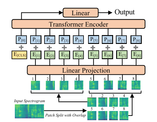
Source: AST: Audio Spectrogram Transformer, Figure 1. The overlap makes patch count a stride calculation.

Reconstructing the AST input ledger

The AST paper specifies 128-dimensional log-Mel filterbank features from a 25 ms Hamming window every 10 ms. It then extracts 16 x 16 spectrogram patches with stride 10 in both dimensions, which means six bins of overlap. For a common 128 x 1024 input:

frequency positions:
    floor((128 - 16) / 10) + 1 = 12

time positions:
    floor((1024 - 16) / 10) + 1 = 101

patch rows:
    12 * 101 = 1,212

This number is not an encoder hyperparameter discovered after preprocessing; it is fixed by the frontend duration/padding and patch policy. The paper’s source-reported overlap ablation makes the tradeoff concrete:

Patch split	Rows	Full AudioSet mAP
no overlap	512	0.451
overlap 2	657	0.456
overlap 4	850	0.455
overlap 6	1,212	0.459

These are paper-specific results, not a universal claim that maximum overlap is best. They show that overlap changes both information coverage and quadratic Transformer work. AST also compares square 16 x 16 patches with temporal 128 x 2 strips: strips restore an explicit temporal ordering, while square patches support transfer from image-pretrained ViT weights. Unit shape and pretraining compatibility are coupled design choices.

def ast_units(waveform, sample_rate, target_frames=1024):
    assert sample_rate == 16_000  # Example checkpoint contract.
    fbank = log_mel_fbank(
        waveform,
        sample_rate=sample_rate,
        n_mels=128,
        window_ms=25,
        hop_ms=10,
    )                              # [B, 128, T]
    fbank, time_valid = pad_or_crop_time(fbank, target_frames)

    patches = fbank.unfold(1, 16, 10).unfold(2, 16, 10)
    # [B, 12, 101, 16, 16] for T=1024
    B, nf, nt, pf, pt = patches.shape
    units = patches.reshape(B, nf * nt, pf * pt)

    freq = torch.arange(nf).repeat_interleave(nt)
    time = torch.arange(nt).repeat(nf)
    geometry = torch.stack([freq, time], dim=-1)
    valid = patch_validity_from_frame_mask(time_valid, 16, 10, nf)
    return units, geometry, valid

Padding policy must propagate into valid. Zero-padded time patches are still finite numeric rows; without a validity mask, the model can treat recording length and padding shape as evidence.

Alternative audio units preserve different evidence:

short frames:
    timing and phonetic detail; long sequences

long chunks:
    efficient summaries; blurred boundaries

speaker turns:
    conversational structure; dependent on diarization

acoustic events:
    semantically sparse; dependent on event detector coverage

learned units:
    data-driven categories as in HuBERT-style pipelines;
    quantizer or clustering policy becomes part of identity

transcript tokens:
    language content; may omit alarms, music, emotion, timing, and speakers

A transcript is therefore not a lossless audio unitization. It is a task-driven projection from sound to words.

---

0x05 Video: row count grows in space and time

Let video be

$$V \in \mathbb{R}^{B \times T \times C \times H \times W}.$$

Frame-patch unitization with temporal sampling stride $S_t$ and spatial patch side $P$ produces approximately

$$N_{\text{video}} = \left\lceil\frac{T}{S_t}\right\rceil \frac{H}{P}\frac{W}{P}.$$

Tubelets instead consume a temporal depth $P_t$ and spatial block $P\times P$:

$$N_{\text{tubelet}} = \frac{T}{P_t}\frac{H}{P}\frac{W}{P}$$

for non-overlapping divisible dimensions. The temporal depth reduces rows by $P_t$ while mixing motion inside each unit.

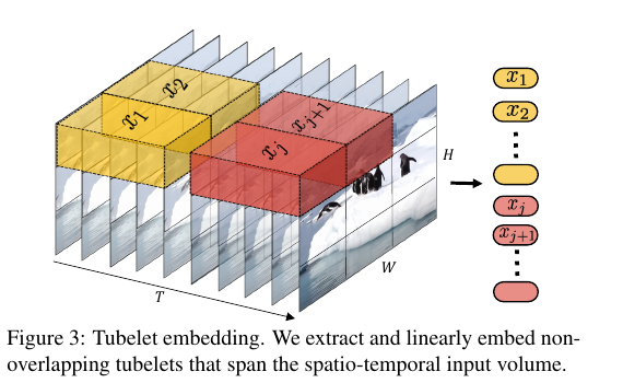
Source: ViViT, Figure 3. A tubelet is explicitly three-dimensional, so its granularity is a joint spatial-temporal choice.

Sampling policy is part of time geometry

If a decoded clip contains $T_{\text{src}}$ frames and the processor requests $n_t$ uniformly spaced observations, one deterministic index policy is

$$i_j= \left\lfloor j\frac{T_{\text{src}}-1}{n_t-1} \right\rfloor, \qquad j=0,\ldots,n_t-1.$$

Another policy starts at a random offset and uses fixed stride; a serving policy may process multiple temporal views. These choices are not equivalent. Uniform endpoint sampling covers the clip but creates nonuniform gaps after rounding. Fixed-stride clips preserve local cadence but can omit the end. Random training clips augment time while making exact replay dependent on the sampled offset and random seed.

@dataclass
class SampledClip:
    frames: Tensor          # [n_t, C, H, W]
    source_index: Tensor    # [n_t]
    timestamp_s: Tensor     # [n_t]
    valid: Tensor           # [n_t]

def sample_uniform(video, timestamps, n_t):
    idx = torch.linspace(0, len(video) - 1, n_t).floor().long()
    return SampledClip(
        frames=video[idx],
        source_index=idx,
        timestamp_s=timestamps[idx],
        valid=torch.ones(n_t, dtype=torch.bool),
    )

Store both source index and timestamp. Variable-frame-rate video breaks the assumption that frame-index distance equals elapsed time.

Tubelet projection is a 3D convolution

For temporal kernel $P_t$, spatial kernel $(P_h,P_w)$, and matching strides, a Conv3d maps each non-overlapping volume to one state. The tensor trace is:

def tubelet_projection(video, d_v, tubelet=(2, 16, 16)):
    # video: [B, T, C, H, W]
    x = video.permute(0, 2, 1, 3, 4)       # [B, C, T, H, W]
    proj = nn.Conv3d(
        x.shape[1], d_v,
        kernel_size=tubelet,
        stride=tubelet,
    )
    grid = proj(x)                          # [B, d_v, nt, nh, nw]
    states = grid.flatten(2).transpose(1, 2)  # [B, nt*nh*nw, d_v]
    return states, grid.shape[-3:]

The flatten order here makes width vary fastest, then height, then time. The origin record for row $s$ must invert that exact order and return a temporal interval plus a spatial rectangle, not only one frame number.

When transferring a 2D image patch kernel $W^{2D}$ to a temporal kernel, ViViT compares three initialization choices:

random:
    initialize the complete 3D kernel from scratch

filter inflation:
    copy W_2D into every temporal slice and divide by P_t

central frame:
    place W_2D in the central temporal slice and initialize other slices to zero

The source-reported Kinetics-400 results for the paper’s comparison were 73.2, 77.6, and 79.2 top-1 respectively. Those values are not universal rankings; they demonstrate that the unitizer’s temporal kernel shape and initialization are part of training compatibility, not merely tensor plumbing.

A one-minute video sampled at two frames per second and patchified at 224 x 224, P=16, produces

$$N=60\cdot2\cdot14^2=23{,}520$$

rows. Dense pairwise interaction would expose

$$N^2 = 553{,}190{,}400$$

logical query-key pairs per head. This derivation explains why video systems sample frames, merge patches, factorize spatial and temporal attention, track objects, or resample features before the language core.

ViViT paper variants: the same units, different interaction topology

Let $n_s=n_hn_w$ be spatial rows per temporal index. Joint attention exposes $(n_tn_s)^2$ logical pairs. Two common factorizations reduce that ledger:

$$C_{\text{factorized self-attention}} \propto n_tn_s^2+n_sn_t^2,$$

while a factorized encoder that summarizes each frame before temporal modeling has the conceptual pair ledger

$$C_{\text{factorized encoder}} \propto n_tn_s^2+n_t^2.$$

ViViT studies four variants rather than one canonical video Transformer:

ViViT variant	Where space and time interact	Main design consequence
Model 1: spatio-temporal	every token attends jointly	earliest global interaction, largest pair matrix
Model 2: factorized encoder	spatial encoder per temporal index, then temporal encoder over summaries	late temporal fusion and fewer temporal rows
Model 3: factorized self-attention	spatial attention then temporal attention inside each block	every block mixes both axes with extra projections
Model 4: factorized dot product	dot-product attention is separated by axis	low compute without the extra encoder of Model 2

For ViViT-B/16x2, the paper reports 455.2, 284.4, 372.3, and 277.1 GFLOPs for Models 1—4, with different accuracy/runtime tradeoffs. These are source-reported measurements on the paper’s setup. X1.1 uses them to show why unit count and axis identity must survive preprocessing; X1.2 owns the encoder topologies themselves.

Frames, tubelets, clips, tracks, and events are not interchangeable:

Unit	Explicit evidence	Main risk
Frames	full sampled scene at a time	event between samples disappears
Frame patches	local spatial evidence over sampled time	row count explodes
Tubelets	short local motion	fine motion mixes inside unit
Clips	longer event summary	boundaries and order can blur
Object tracks	identity over time	tracking errors break continuity
Events	sparse semantic changes	event detector defines recall

For “what did the person pick up after opening the drawer?”, tracks or dense temporal evidence make object continuity explicit. Sparse independent frames force the model to solve tracking again from the retained samples.

---

0x06 Tool, event, and action units

Tools begin with structure that is often accidentally discarded:

{
  "type": "tool_call",
  "name": "browser.click",
  "args": {"x": 412, "y": 293},
  "timestamp": "2026-07-17T09:41:00Z",
  "status": "requested",
  "parent_call_id": "turn_17"
}

Three choices are common.

serialize to text:
    easy reuse of text tokenizer and language model
    field boundaries and numeric geometry become tokenization-dependent

typed field units:
    event type, tool name, arguments, status, time, and authority stay explicit
    requires field encoders and a stable schema

discrete action tokens:
    continuous action chunks become IDs
    quantizer precision and decoding contract become part of control safety

For a typed event, unit identity can be represented as

$$u_i=(\text{event type},\text{field},\text{value},\text{time},\text{parent},\text{status}).$$

Dropping status or parent preserves plausible text while changing causal meaning. This is the structured-I/O analogue of detaching a box from its OCR span.

Continuous actions add another design axis. FAST transforms an action chunk by normalization, a discrete cosine transform, scalar quantization, frequency-first flattening, and BPE compression.

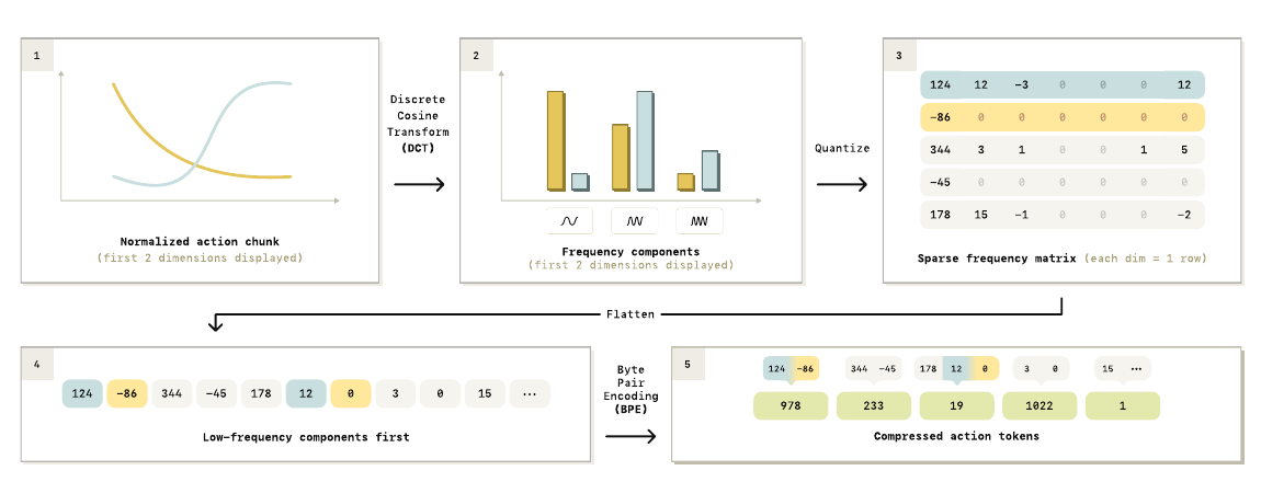
Source: FAST, Figure 4. Every stage changes the action-token contract: transform basis, quantization resolution, coefficient order, and vocabulary merges.

Why per-timestep bins become a poor target at high control rates

Suppose a smooth action dimension is sampled every $\Delta t$. A first-order expansion gives

$$a(t+\Delta t)-a(t) =a'(t)\Delta t+O(\Delta t^2).$$

As control frequency rises, $\Delta t$ shrinks and adjacent values increasingly fall into the same quantization bin. The next token carries little marginal information beyond the previous token even though the complete trajectory may still encode a difficult dexterous motion. FAST’s motivating experiment holds the underlying spline distribution fixed while increasing samples from 25 to 800 steps; naive per-timestep binning becomes progressively harder for the autoregressive policy. The problem is the target representation, not a more complex physical trajectory.

Frequency coefficients allocate units differently. Low-frequency coefficients describe the chunk’s broad shape; higher frequencies add corrections. Predicting low frequencies first therefore exposes high-information decisions before local details, which is why FAST uses frequency-first rather than dimension-first flattening.

Deriving the FAST codec and its error boundary

For an action chunk $A\in\mathbb{R}^{H\times D}$, first normalize each action dimension using training-set quantiles $q_{0.01,d}$ and $q_{0.99,d}$:

$$\widetilde A_{t,d} =2\frac{\operatorname{clip}(A_{t,d},q_{0.01,d},q_{0.99,d})-q_{0.01,d}} {q_{0.99,d}-q_{0.01,d}}-1.$$

Quantile normalization is robust to occasional outliers, but clipping is lossy and the statistics are robot/action-schema specific. Next apply an orthonormal DCT-II independently along time:

$$C_{k,d} =\alpha_k\sum_{t=0}^{H-1} \widetilde A_{t,d} \cos\left[\frac{\pi}{H}\left(t+\frac12\right)k\right],$$

with $\alpha_0=1/\sqrt H$ and $\alpha_k=\sqrt{2/H}$ for $k>0$. Quantization is

$$Q_{k,d}=\operatorname{round}(\gamma C_{k,d}), \qquad \widehat C_{k,d}=Q_{k,d}/\gamma.$$

Ignoring clipping, each coefficient’s rounding error is bounded by $1/(2\gamma)$. Because the orthonormal DCT preserves the Euclidean norm, the coefficient-domain reconstruction error is the action-domain normalized error:

$$\|\widehat A-\widetilde A\|_F =\|\widehat C-C\|_F.$$

This is why $\gamma$ has a direct rate-distortion interpretation. Larger $\gamma$ reduces rounding error but creates a less sparse, harder-to-compress integer stream. BPE then compresses that stream losslessly relative to $Q$. It does not undo DCT quantization or clipped normalization.

The integer order is frequency-major:

$$[Q_{0,0},Q_{0,1},\ldots,Q_{0,D-1}, Q_{1,0},\ldots,Q_{H-1,D-1}].$$

This serialization places the coarse trajectory components before the details. BPE merges frequent integer subsequences, including runs of zeros, into a fixed action vocabulary that can be allocated inside a VLM vocabulary.

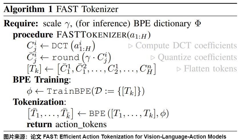
Source reused from Transformer Series A6, reproducing FAST Algorithm 1.

@dataclass(frozen=True)
class FastManifest:
    horizon: int
    action_dim: int
    q01: Tensor
    q99: Tensor
    dct_type: int
    dct_norm: str
    gamma: float
    flatten_order: str
    bpe_vocab_hash: str
    token_id_offset: int

def fast_encode(actions, manifest, bpe):
    # actions: [B, H, D]
    assert actions.shape[1:] == (manifest.horizon, manifest.action_dim)
    normalized = quantile_normalize(actions, manifest.q01, manifest.q99)
    coeff = dct(normalized, axis=1, type=2, norm="ortho")
    integers = torch.round(manifest.gamma * coeff).to(torch.int32)
    # DCT axis first, then action dimension: low frequencies enter BPE first.
    stream = integers.reshape(actions.shape[0], -1)
    tokens = bpe.encode_integer_stream(stream) + manifest.token_id_offset
    return tokens

def fast_decode(tokens, manifest, bpe):
    stream = bpe.decode_integer_stream(tokens - manifest.token_id_offset)
    q = stream.reshape(-1, manifest.horizon, manifest.action_dim)
    coeff = q / manifest.gamma
    normalized = idct(coeff, axis=1, type=2, norm="ortho")
    return quantile_denormalize(normalized, manifest.q01, manifest.q99)

The paper reports two tokenizer hyperparameters for its single-dataset setup: rounding scale 10 and BPE vocabulary size 1024. They are source-reported design choices, not constants that should be silently baked into every robot policy. FAST+ additionally trains a universal BPE vocabulary from cross-embodiment trajectories; the normalization statistics and action schema remain runtime inputs to compatibility.

Action representation alternatives

Method	Prediction unit	Strength	Main failure boundary
Per-step scalar bins	one categorical ID per dimension and timestep	simple and directly autoregressive	long redundant sequences at high control rate
Vector quantization	learned code for a vector/chunk	data-adaptive nonlinear codebook	codebook training, collapse, and dataset binding
FAST	BPE tokens over quantized DCT coefficients	analytic transform, short sequences, fast inverse	clipping/rounding error and strict manifest identity
Continuous regression	real-valued action or chunk	preserves metric output directly	multimodality can average incompatible actions
Diffusion/flow action head	iterative continuous trajectory	expressive multimodal output	different loss, scheduler, and latency contract

These are architecture choices, not interchangeable tokenizers. Replacing a continuous action head with FAST changes output vocabulary, labels, stopping rules, detokenization, and control latency. X1.3 owns the resulting training and runtime state, but X1.1 must emit the manifest that makes inversion safe.

This does not imply that every action should be tokenized. Continuous regression preserves metric geometry; categorical actions simplify sequence modeling; transformed tokens compress smooth trajectories. The runtime must know which decoder reverses the chosen representation.

---

0x07 One batch needs more than a feature tensor

A robust multimodal unitizer should not return only features. It should return a typed bundle:

@dataclass
class UnitBatch:
    values: Tensor              # [B, N, d_raw] or IDs [B, N]
    valid: Tensor               # [B, N]
    modality: Tensor            # [B, N]
    unit_kind: Tensor           # [B, N], e.g. patch/span/tubelet/action ID
    origin_id: Tensor           # [B, N]
    position_1d: Tensor | None  # [B, N]
    boxes_2d: Tensor | None     # [B, N, 4]
    time_span: Tensor | None    # [B, N, 2]
    page_id: Tensor | None      # [B, N]
    track_id: Tensor | None     # [B, N]
    source_transform: Tensor | None  # [B, 3, 3], when geometry is affine
    processor_manifest_hash: str

The exact fields differ by modality, but four invariants should be executable:

def validate_units(batch: UnitBatch):
    B, N = batch.valid.shape
    assert batch.values.shape[:2] == (B, N)
    assert batch.modality.shape == (B, N)
    assert batch.unit_kind.shape == (B, N)
    assert batch.origin_id.shape == (B, N)

    for metadata in [batch.position_1d, batch.page_id, batch.track_id]:
        if metadata is not None:
            assert metadata.shape == (B, N)

    if batch.boxes_2d is not None:
        assert batch.boxes_2d.shape == (B, N, 4)
    if batch.time_span is not None:
        assert batch.time_span.shape == (B, N, 2)

    # Padding must not claim a real origin.
    assert torch.all(batch.origin_id[~batch.valid] == -1)

Use $N_u$ for this row count. It is deliberately distinct from X1.2’s encoder row count $N_e$ and language-visible row count $N_l$:

X1.1: U_raw      [B, N_u, d_raw]  plus aligned metadata
X1.2: H_encoded  [B, N_e, d_enc]
X1.2: Z_language [B, N_l, d_model]

N_e may differ because an encoder merges or adds rows. N_l may differ because a resampler chooses a fixed query budget. X1.1 must not pre-label its raw patch vectors as language tokens or encoded features.

The dataclass is a homogeneous per-modality interface. Image patch vectors and audio patch vectors need not share d_raw; a mixed request should carry a dictionary of typed UnitBatch objects until modality-specific encoders and projectors produce a compatible width. Padding unrelated raw modalities into one largest-width tensor creates a superficially unified API and an ambiguous checkpoint contract.

Origin maps are a debugging primitive

origin_id should survive crop, sample, split, merge, pad, encode, and project. For an image patch it may point to (image_id,row,col,scale). For OCR it may point to (document_id,page,span_id). For video it may point to a frame interval and spatial box. When the final model attends to or fails on a row, the origin map provides a path back to the raw evidence.

Without that map, a tensor-level failure often ends at “row 137 looked wrong.”

Training and serving must bind the same processor manifest

Model weights do not identify the preprocessing path by themselves. A unitizer artifact should version every value that changes units, geometry, or decoding:

processor_manifest = {
    "schema_version": 3,
    "modality": "video",
    "decoder": {"library": "...", "version": "..."},
    "temporal_sampling": {"method": "uniform", "frames": 32},
    "spatial": {"resize": 256, "crop": 224},
    "tubelet": {"kernel": [2, 16, 16], "stride": [2, 16, 16]},
    "flatten_order": "time-height-width",
    "normalization": {"mean": [...], "std": [...]},
    "metadata_schema": "unit-batch-v3",
}
processor_manifest_hash = canonical_json_sha256(processor_manifest)

The cache key must include that hash:

$$k_{\text{unit cache}} =H(\text{raw-object digest},\text{processor-manifest hash}).$$

Keying only by image/video bytes can return rows produced by an older resize, patch, sample, or normalization policy. A dimension check may still pass if the new and old policies happen to produce the same $N_u$.

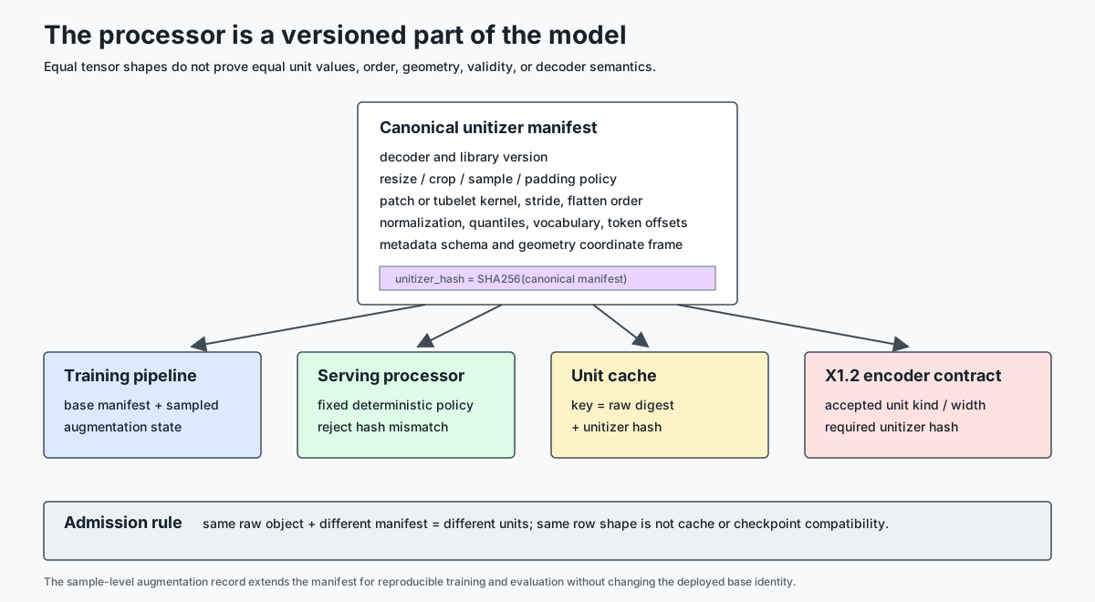
Runtime admission should reject rather than guess:

def admit_unit_batch(batch, encoder_contract):
    assert batch.processor_manifest_hash == encoder_contract.unitizer_hash
    assert batch.values.shape[-1] == encoder_contract.raw_unit_width
    assert batch.valid.dtype == torch.bool
    real_kinds = batch.unit_kind[batch.valid]
    assert torch.isin(real_kinds, encoder_contract.accepted_unit_kinds).all()

Augmentations complicate identity during training. Random crop, time shift, SpecAugment, frame jitter, and OCR masking should be recorded as sample-level transform state derived from a stable base manifest. Serving disables or fixes those stochastic transforms. Reproducible evaluation records the random seed or materialized transform parameters with each sample.

---

0x08 Sequence, compute, and information ledgers

The total language-visible row count can be written as

$$N_{\text{total}} = L_{\text{text}} +N_{\text{image}} +N_{\text{document}} +N_{\text{audio}} +N_{\text{video}} +N_{\text{event}}.$$

This is a bookkeeping identity, but it has runtime consequences. If all rows enter one dense self-attention sequence, the score matrix contains $N_{\text{total}}^2$ logical entries per head. If media remains separate memory, cross-attention has approximately $L_{\text{text}}N_{\text{media}}$ scores. If a resampler converts $N_{\text{media}}$ rows to $Q$ learned latents, the language-visible interaction becomes $L_{\text{text}}Q$, plus the resampler’s own cost. X1.2 derives those fusion choices.

The relevant ledgers must remain separate:

Ledger	Question
Raw units	What evidence did preprocessing expose?
Encoder rows	How many states did the modality encoder produce?
Language-visible rows	How many rows reach the language computation?
Metadata bytes	What boxes, timestamps, masks, and origin maps remain resident?
Pair count	Which rows can interact under the chosen fusion topology?
Information loss	Which task-relevant distinctions disappeared upstream?

A reduction from 4,096 image patches to 64 learned latents is a 64-fold sequence reduction and a 4,096-fold reduction in a self-attention pair count for that block. It is also an information bottleneck whose loss must be tested on small text, localization, counting, and rare-detail tasks.

---

0x09 Geometry alternatives and handoff to M3

Preserving geometry does not prescribe one positional mechanism. A unitizer can expose:

absolute sequence index
2D or 3D coordinates
bounding boxes
relative offsets
page / segment / modality IDs
timestamps and durations
track identity
hierarchical parent-child links

The model may then use additive position embeddings, attention bias, rotary geometry, coordinate features, or a combination. M3.3 owns the mathematical positional families. X1.1 owns the upstream invariant:

Geometry can only be encoded if the preprocessing path preserved and aligned it with unit identity.

Flattening a 2D grid into 1D order is not inherently wrong. It is wrong when the model and metadata disagree about the flattening, when multiple images reuse coordinates without boundaries, or when crops and tiles lose their global origin.

---

0x0A Failure lab

Failure	Tensor symptom	Semantic damage	Required check
Patch order mismatch	valid [B,N,d]	coordinates point to other pixels	reconstruct a test image from ordered patches
Crop/box mismatch	valid boxes and pixels	OCR/region geometry shifted	replay all transforms on boxes
Coarse image units	low N	tiny text or objects absent	stratify evaluation by evidence size
Fine image units	high N	prefill/memory budget exceeded	log rows at every stage
Transcript-only audio	normal text IDs	non-speech and timing evidence absent	retain audio/event path where task requires it
Audio frontend drift	same [B,F,T] rank	values and time-frequency coordinates change	bind sample rate, window, hop, Mel bank, padding, and normalization
Video sampling gap	valid sampled frames	key event never observed	temporal coverage audit
Variable-frame-rate indexing	valid frame IDs	frame distance is mistaken for elapsed time	retain decoded timestamps
Broken tracks	valid track tensor	identity swaps across time	track continuity tests
Ragged padding visible	mask mismatch	PAD units become evidence	assert padded rows are masked
Metadata permutation	compatible shapes	features and metadata describe different units	carry origin IDs through every permutation
Tool record flattening	plausible token sequence	status, authority, or parent relation lost	typed schema round-trip
Action quantization too coarse	valid IDs	control precision unavailable	decode-error and task-safety thresholds
FAST manifest mismatch	valid action-token IDs	wrong scale, BPE vocabulary, shape, or robot normalization	hash and admit the complete tokenizer manifest
Unit cache staleness	correct row shape	rows come from an older processor	include manifest hash in cache key
Placeholder count mismatch	text/media lengths differ	media states inserted at wrong positions	X1.3 expansion invariant

The common pattern is important: most of these failures preserve tensor rank. Shape checks catch interface errors; origin and semantic checks catch representation errors.

---

0x0B Handoff to X1.2

After X1.1, the system has units and aligned metadata:

image patches / regions / OCR spans
audio frames / spectrogram patches / learned units
video frames / tubelets / tracks
typed events / action chunks / action IDs
validity masks and origin geometry

These are not yet necessarily language-model states. X1.2 asks how a modality encoder produces feature states, how a projector aligns feature width and space, how a resampler changes row count, and whether the language core receives media as prefix rows, interleaved rows, or cross-attention memory.

The concrete boundary is:

X1.1 emits:
    raw unit values U                       [B, N_u, d_raw] or [B, N_u] IDs
    row validity V                         [B, N_u]
    unit kind and modality                 [B, N_u]
    origin and geometry aligned to N_u
    processor manifest hash

X1.2 consumes:
    one homogeneous UnitBatch per modality
    an encoder contract bound to the same processor manifest

X1.2 may produce:
    encoded rows H                         [B, N_e, d_enc]
    language-visible rows Z                [B, N_l, d_model]

No X1.2 projector may infer grid shape from $\sqrt{N_u}$ when class tokens, padding, non-square inputs, tiles, or tubelets are possible. It must consume the explicit geometry or the serialized grid shape.

The final X1.1 invariant is:

If evidence is not preserved as a unit or aligned unit metadata, later encoders and attention cannot reliably recover it.

---

0xFF References

• An Image is Worth 16x16 Words
• LayoutLM
• LayoutLMv3
• Donut
• Pix2Struct
• wav2vec 2.0
• HuBERT
• Whisper
• Audio Spectrogram Transformer
• ViViT
• TimeSformer
• VideoMAE
• FAST: Efficient Action Tokenization
• Large Concept Models: Language Modeling in a Sentence Representation Space
• Transformer Series (6) - Token
• Transformer Series (7) - Embedding
• Transformer System M2.1 - Text Tokenization
• Transformer System M2.2 - Embeddings and Projectors
• Transformer System M3.3 - Position Encoding and Context Geometry
• X1.2 - Multimodal Encoders, Projectors, Resamplers, and Fusion