M1.1 — Why Transformers, Which Architecture, and What Executes

The preface situates this technical study within the two connected programs, Transformer System and Autonomous Agents.

0x00 From A Sentence To A Sequence Model

Modeling a sequence requires more than assigning a representation to each item. A prediction may depend on information several positions away, and the task determines which information it may use. In translation, source and target can differ in length and word order; during autoregressive generation, the available output prefix grows one token at a time.

Recurrence, convolution, and attention provide different answers to this information-access problem. They differ in where earlier information is stored, how a prediction reads it, and which operations depend on the completion of previous ones. These choices shape both the functions the model can learn and the parallelism available during training and inference.

To understand the Transformer, we will reconstruct these alternatives before assembling its components into a complete model. We will then trace the connection between that architecture, the objects that own its parameters, and the tensors used in execution. We begin with a minimal contextual distinction: changing one word can alter which continuation should be considered plausible.

0x00A What The Context Changes

Consider two short passages:

The report was convincing. The committee …

The report was not convincing. The committee …

The shared words are not enough to interpret these passages. The presence of “not” changes the meaning of the first sentence and can change the relative plausibility of continuations such as “accepted the proposal” and “rejected the proposal.” It does not determine what the committee actually did. A language model must represent uncertainty as well as respond to context.

Now insert several sentences about the report’s methods before the committee’s decision. The relevant information is still present, but a model that only examines the last few words may no longer have access to it. In a translation, losing the negation can produce a fluent sentence with the wrong meaning. In continuation, overlooking it can make the prediction insensitive to a distinction it should be able to use.

This is a small example of a consequential failure: the output can look well formed while no longer saying what the source says. To investigate it, we need more than a judgment that the answer is bad. We need to follow the negation from the input into a representation and then into the prediction. Was the relevant information available to that prediction? Did the learned computation use it? Those are different questions, and they lead to different experiments.

This gives the architecture a problem to solve. It must handle different sequence lengths, distinguish order, and reuse learned relationships across positions. It must also let a prediction draw on relevant information that may not be adjacent to it. Simon Prince develops these sequence-modeling requirements in Chapter 12 of Understanding Deep Learning.

Before choosing an architecture, however, we need to understand what it operates on. A machine does not receive “the meaning of the report” as an input. It receives an encoded sequence. Learning must make that sequence useful for a task; the architecture must provide a path from the resulting representations to each prediction.

0x00B Why Learn A Representation?

A predictor that keeps a separate answer for each complete passage has no answer ready when that passage changes. We would like examples to teach it relationships that can also influence other predictions. Neural language models make this possible through shared learned representations and transformations: an example can change coefficients that are used again on other inputs, rather than only update a record for that exact sentence. Learning a representation and a probability function together was already central to neural language modeling before the Transformer. (Bengio et al., 2003)

Sharing is useful only when what is shared helps the task. Two passages can use almost the same vocabulary while differing in a crucial negation. A good representation must let the predictor reuse helpful relationships without erasing that distinction. It is therefore not enough to say that a network turns text into numbers. We need to ask what those numbers let the next computation distinguish and combine.

Text does not enter a neural network as a sentence whose meaning is already available. A tokenizer divides it into units and assigns integer IDs. Depending on the tokenizer, a unit may be a word, part of a word, a byte, or another vocabulary entry. An ID is an index, not a numerical measure of meaning: token 200 is not “twice as meaningful” as token 100.

An embedding maps each ID to a learned vector. With an embedding table, occurrences of the same token ID begin with the same looked-up vector. Later computations combine this representation with position and permitted context, so the resulting state can differ between occurrences. The initial embedding does not already contain the meaning of the whole sentence, and its coordinates do not come with guaranteed human-readable meanings.

A vector is a list of numbers; a matrix arranges numbers in rows and columns. Tensor is the more general term for an array with indexed axes: a vector has one axis, a matrix has two, and a batch of vector sequences has three. These arrays give us a concrete way to implement the transformations. Whether the learned transformations preserve a negation or transfer to a new writing style remains something to evaluate.

For the report example, recognizing the token “not” is only the beginning. Its effect depends on the statement it qualifies. A useful intermediate state must allow later computations to distinguish the two passages, even though most of their token IDs are identical. This is the reason for learning representations rather than treating tokenization as the end of the problem.

0x00C Learning And Using The Model

The distinction between learning across examples and using the current passage now has a numerical form. Parameters are the coefficients reused across examples, such as embedding-table entries and projection weights. Activations are intermediate results computed for the current input. Training changes parameters; an ordinary inference call holds them fixed and produces new activations.

To train a next-token predictor, an example supplies both a prefix and the token that follows it. The model produces a prediction from the allowed context, and a loss measures how poorly that prediction fits the supplied target. Derivatives describe how parameter changes would affect the loss; an optimizer uses them to adjust the parameters. A low training loss alone does not establish that the model will handle a new passage well. We also need evaluation examples that test the behavior we actually want.

The target token is one observed continuation, not necessarily the only reasonable one. Predicting a distribution lets the model assign different probabilities to alternatives. Training can reward a supplied continuation without giving us a rule that every other continuation is false. In translation, several phrasings may preserve the source meaning; in our report example, a phrasing that removes the negation changes that meaning instead.

The way we present the example is part of the learning problem. If a prediction can read the very answer it is meant to predict, its training results may look excellent without teaching the intended behavior. Supplying the answer as a label for comparison is different from revealing it as an input to that prediction. We will make this distinction precise through the input shift and the attention mask.

For next-token prediction, the final representation is mapped to one score per vocabulary entry. These unnormalized scores are logits. A softmax converts them into probabilities; a decoding policy then chooses a token. The broad path is:

source bytes
    -> token IDs and sequence metadata
    -> initial state rows
    -> encoder and/or decoder block stacks
    -> vocabulary logits
    -> compare with supplied labels (training)
       or select token IDs and continue (generation)

The two branches use the same kind of prediction differently: training compares it with a supplied label, while generation must choose what comes next. The labels are not produced by the logits.

At generation time, there is no supplied next label to compare against. A procedure must choose a token, append it to the prefix, and ask the model for another prediction. Follow the changing input in the illustration:

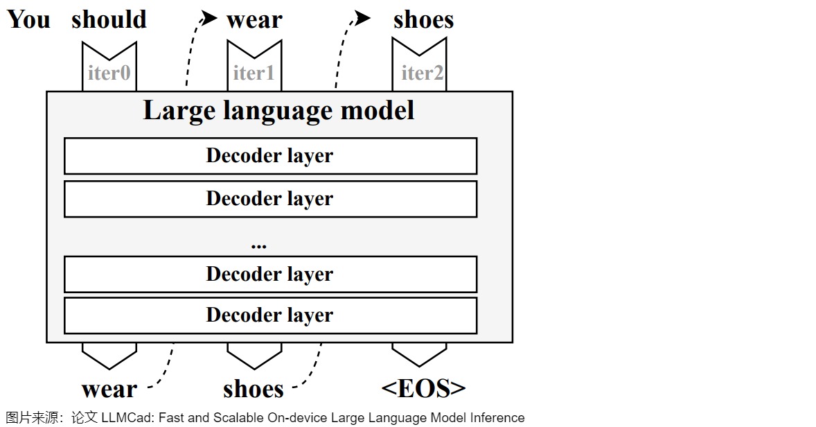
Autoregressive generation, illustrated in LLMCad. “You should” first becomes “You should wear” and then “You should wear shoes”. Each new prediction uses the earlier choice as part of its input; the last choice is an end-of-sequence symbol. Words stand in for tokens here: an actual tokenizer may split them differently. This is a generation loop, not a claim that every Transformer is decoder-only or that training evaluates only one position at a time.

Adding another token changes the input and runtime state; it does not, by itself, update the weights. Choosing the most probable token and sampling from the distribution are different decoding policies. Neither turns a probable continuation into a guarantee of truth, nor replaces the training that produced the model’s probabilities.

0x00D Why Architecture Matters

Token IDs, embeddings, and a training objective do not yet specify how information moves between positions. In the report example, the computation that predicts the committee’s decision needs some way to use the earlier assessment. A recurrent model can carry a state from one position to the next. A convolution can combine local neighborhoods, with deeper layers extending the range. Attention can compute weights from representations and combine information from the positions it is permitted to read. These are different ways to arrange information paths, with different costs and constraints.

The original Transformer used attention in place of recurrent or convolutional sequence updates in its encoder-decoder. Many computations over known positions could therefore run in parallel, while autoregressive generation still had to wait for previously selected output tokens. (Vaswani et al., 2017)

This makes it useful to distinguish an architecture from a trained model. The architecture specifies available transformations and information paths. The trained model also contains parameter values obtained by training on particular data with a chosen optimization procedure. Two models can share an architectural design without acquiring the same capabilities. Providing a path from a distant word to a prediction makes a dependency available; it does not guarantee that training will teach the model to use it well.

Nor does every Transformer have to generate text. A language model assigns probabilities to language sequences; a Transformer is one family of architectures with which such a model can be built. Language is our starting example, not a restriction on the architecture’s possible inputs or tasks. Classifying a document needs a category; locating an answer may need a span; generating a translation needs a sequence and a stopping decision. These tasks can share representation machinery without sharing an output head. They do not uniquely determine an architecture either: T5, for example, expresses different tasks through a text-to-text interface. (Raffel et al., 2020)

The value of architectural understanding is being able to trace such choices. If a translation loses the negation, we can investigate whether the relevant input was available, how it was represented, and whether the learned model uses it. We do not have to treat every failure as evidence that an unspecified “larger model” is needed.

0x00E Making The Computation Practical

Suppose the passage grows into a long document. Splitting it into independent fragments may reduce resource use, but removes context across the boundaries. Letting every position attend to every other permitted position preserves more possible information paths, but introduces work that grows with the number of position pairs. The information we want the model to use and the computation we can afford are connected design problems.

There is more than one way to respond. We could restrict the attention pattern, changing which information is available. Or we could preserve the attention computation and change how it is executed. FlashAttention, for example, reorganizes exact attention into blocks to reduce transfers between levels of GPU memory. It does not replace attention with an approximate rule, although results in finite precision can differ with the order of computation. Changing what the model computes and changing how the machine computes it are different interventions.

Training introduces another constraint. A model that fits in memory for prediction may not fit when training requires saved activations, gradients, and optimizer state. Resource limits affect which experiments we can run and which adaptations we can attempt. A failure to learn the task and a failure to fit its training computation in memory need different explanations and different remedies.

Serving introduces a workload rather than just one example. When one document becomes many simultaneous requests, we care about waiting time and how much work the hardware can sustain. Processing requests together can improve hardware use, but changes memory demand and scheduling. In autoregressive serving, even the management of saved intermediate state can limit how many requests fit at once, as the PagedAttention paper demonstrates.

A Transformer system therefore includes more than a trained model. It includes preparing data, performing updates, executing computations, constructing outputs, evaluating behavior, and managing resources. We may train from the beginning, adapt existing weights, or use a model unchanged; each choice leaves different parts of that work to do. Engineering here includes the learning and modeling decisions, not just an interface around fixed weights.

An apparently fluent translation can still mishandle negation, terminology, or writing styles absent from its training. Faster execution cannot repair that by itself, and a more capable model does not remove memory limits or waiting time. Useful capability and practical computation have to be developed together. Understanding their connection lets us choose what to change and what to measure. A claim of “faster” needs a workload; a claim of “smaller” needs us to ask which state became smaller and what happened to the result.

0x00F From The Problem To The Running Model

We now have a reason to look inside the model. A translation must preserve useful distinctions in its input, construct a well-formed output, and do so with a computation we can train and run. The Transformer brings together several design choices that address these demands. Understanding those choices is easier if we first build a smaller model and ask where its information has to travel.

Our first model will read a source sequence into one learned summary and use that summary to generate a translation. This is a complete, trainable idea, not an intentionally broken predecessor. Its limitation becomes clearer when different output positions need different details from the source. That will give us a concrete reason to investigate attention before assembling the Transformer.

Basic probability, vectors, matrix multiplication, and derivatives will help with the derivations. Each new tensor comes with a role and dimensions, and the small numerical traces make the operations inspectable. We begin one step before the architecture: what probability should a model assign to a complete translation, and how can it learn to assign that probability?

0x01 How A Model Assigns Probability To A Sequence

For the report passage, we want a translation that preserves the relationships between statements, not just a sequence of plausible words. Even a much shorter example shows why translation cannot be a collection of independent word replacements: “Thank you” can become “Merci”. The output has its own length and order, and more than one translation may be acceptable. A model must assign probabilities to complete possible outputs, then a generation procedure must construct one and decide when to stop.

We can state this precisely before choosing a neural architecture. Let

$$X=(x_1,\ldots,x_{T_x}), \qquad Y=(y_1,\ldots,y_{T_y}),$$

Here the lowercase symbols denote tokens; $T_x$ and $T_y$ are their source and target counts, which may differ. The vertical bar in $P(Y\mid X)$ means “given this source.” It distinguishes a translation model from a model that merely prefers fluent target sentences without considering what they translate.

0x01A Variable Length Requires A Stop Event

Producing “Merci” is not yet the same event as producing “Merci” and stopping. The first could also be the beginning of a longer answer. To assign a probability to a completed sequence, the model needs a stopping event as well as probabilities for the preceding tokens.

The shorthand $P(Y\mid X)$ hides the decision to stop. Introduce a beginning symbol $y_0=\langle\mathrm{BOS}\rangle$ and define $y_{T_y+1}=\langle\mathrm{EOS}\rangle$. The modeled event is then

$$p(y_1,\ldots,y_{T_y},\langle\mathrm{EOS}\rangle\mid X).$$

BOS supplies a starting input before the first target token exists; it is not a translated word. EOS, by contrast, is an output the model can predict. The decoder does not need an independently supplied target length at generation time: emitting EOS is part of the distribution. A maximum length or other stopping rule may still be imposed by a runtime, but that is a serving policy rather than the probability factorization.

These choices answer different questions. Asking for a translation tells us the task, but not yet the network. Choosing left-to-right prediction tells us what each prediction can condition on, but not whether a training batch can evaluate many known positions together:

Choice	What it specifies	What it leaves open
Task	map a variable-length $X$ to a distribution over variable-length $Y$	RNN, CNN, or Transformer
Factorization	choose how the joint target probability is decomposed	the neural network used for each factor
Execution	evaluate known target rows during training or discover unknown rows during generation	whether every architecture can evaluate those rows in parallel

Sequence-to-sequence is the task family. Autoregression is one factorization and generation order. Encoder-decoder is an architectural boundary. None is an alias for the other two.

0x01B Deriving The Autoregressive Product

We can replace the difficult problem of scoring a whole output at once with a sequence of conditional questions: how probable is its first token, then its second given the first, and so on? This decomposition follows from the conditional chain rule. Split the first event from the remaining events, then apply the same rule to what remains. For a three-token target plus EOS,

$$\begin{aligned} p(y_1,y_2,y_3,\mathrm{EOS}\mid X) &=p(y_1\mid X)\, p(y_2,y_3,\mathrm{EOS}\mid y_1,X)\\ &=p(y_1\mid X)\, p(y_2\mid y_1,X)\, p(y_3,\mathrm{EOS}\mid y_1,y_2,X)\\ &=p(y_1\mid X)\, p(y_2\mid y_1,X)\, p(y_3\mid y_1,y_2,X)\, p(\mathrm{EOS}\mid y_1,y_2,y_3,X). \end{aligned}$$

Repeating the same split gives

$$p(Y,\mathrm{EOS}\mid X) = \prod_{t=1}^{T_y+1} p(y_t\mid y_{<t},X).$$

In plain notation:

p(Y, EOS | X) = product over t=1..T_y+1 of p(y_t | y_<t, X)

At each factor, the source stays available while the target prefix grows. Multiplication combines these conditional probabilities into the probability of that particular complete path. This does not assume that neighboring target tokens are independent, or that choosing the largest probability at each step must find the most probable complete sequence.

The equality is a probability identity, not an RNN invention. An RNN, a convolutional decoder, and a causally masked Transformer can parameterize the same factors. Conversely, a non-autoregressive model may deliberately use a different approximation, such as conditionally independent target positions plus a length model. That changes the dependency contract; it is not obtained merely by executing the same graph faster.

The identity tells us how to factor a distribution; it does not tell us the probabilities. A neural model with parameters $\theta$ supplies estimates for the factors. Training by maximum conditional likelihood tries to increase the probability it assigns to an observed pair $(X,Y)$.

Why does this become a sum of losses? The logarithm is increasing, so maximizing a positive probability also maximizes its logarithm. The logarithm turns a product into a sum; the minus sign converts maximization into minimization. Taking the negative log of the modeled sequence probability gives

$$\begin{aligned} -\log p_\theta(Y,\mathrm{EOS}\mid X) &=-\log\!\left[\prod_{t=1}^{T_y+1} p_\theta(y_t\mid y_{<t},X)\right]\\ &=-\sum_{t=1}^{T_y+1}\log p_\theta(y_t\mid y_{<t},X). \end{aligned}$$

This is the negative log-likelihood loss for one observed sequence:

$$\mathcal{L}_{\mathrm{NLL}}(X,Y) =- \sum_{t=1}^{T_y+1} \log p_\theta(y_t\mid y_{<t},X).$$

Every term asks how much probability the model gave the supplied token at that position, including EOS. With a single target token as the label, this is the familiar cross-entropy loss against that label. Adding the terms trains the whole sequence, rather than rewarding only its last word.

During teacher-forced training, $y_{<t}$ is the observed target prefix. During generation, it is the prefix selected by the model and decoding policy. For the short translation, suppose that “Merci” is one target token:

Prediction	Teacher-forced input	Label compared with the prediction	Generation-time difference
first target token	source plus BOS	Merci	the decoder chooses a token; it is not supplied Merci in advance
termination after that token	source plus BOS and Merci	EOS	this prefix is reached only if the previous choice was Merci

The factorization is shared; the available prefix and execution schedule differ. We return to this difference in the training and generation examples below; it becomes a complete training program in M3.9.

0x01C Where An Encoder-Decoder Enters The Equation

We have defined a training signal, but not the computation that earns it. Each factor needs information from the source and the target prefix. An encoder-decoder divides this work into two parts: the encoder computes a representation of the source, and the decoder uses it while predicting the target. That representation is the information passed between them.

Call it $Z$. To distinguish the distribution we would like to learn from the model we can implement, write the desired conditional distribution as $p_*$ and the parameterized decoder as $p_\theta$:

$$Z=\operatorname{Encoder}_\theta(X), \qquad p_*(y_t\mid y_{<t},X) \approx p_\theta(y_t\mid y_{<t},Z).$$

The approximation concerns how well the model captures the desired distribution. It is not an approximate substitution inside the implemented network: if the decoder receives source information only through $Z$, that dependence is exact for its computation. What training does not guarantee is that $Z$ preserves everything needed to model the desired predictions well.

For our two report passages, the encoder must produce representations that let the decoder respond differently to the negation. If it produces exactly the same $Z$ for both, a decoder receiving the same target prefix has no remaining way to distinguish them. This makes the choice of representation an architectural decision, not just a name for an intermediate tensor:

Source interface $Z$	Decoder-visible object	Source-access contract
fixed context	one vector $c\in\mathbb{R}^{d_c}$	every target step receives the same source summary
fixed slots	a small, source-length-independent set of vectors	more summary capacity, but no row-per-source interface
addressable annotations	$H=(h_1,\ldots,h_{T_x})$	a target step may construct a new read from source rows

The first two interfaces remain useful design choices. The third retains a separate row for each source position, allowing the decoder to change its source read from one target step to another. Before deriving those read weights in Section 0x04, we can build the one-summary version and inspect exactly what it makes available.

0x01D The Fixed-Vector Recurrent Prototype

A simple recurrent encoder reads one source token at a time. At each step, it combines the new token’s embedding with a state carried from the previous step. “Hidden state” here means an internal numerical result, not an extra label supplied by the data. The same learned update is reused along the sequence:

$$e_i=E_x[x_i], \qquad h_i=f_{\mathrm{enc}}(h_{i-1},e_i), \qquad c=\phi(h_1,\ldots,h_{T_x}).$$

The lookup $E_x[x_i]$ supplies the current token vector, $f_{\mathrm{enc}}$ updates the accumulated state, and $\phi$ chooses the source representation that will reach the decoder. In the report passage, any contribution from “not” must survive through these updates if only the final state is exported.

In the canonical final-state prototype, $\phi(H)=h_{T_x}$, possibly followed by a projection. The decoder then reuses that context:

$$s_t=f_{\mathrm{dec}}(s_{t-1},E_y[y_{t-1}],c), \qquad \ell_t=W_o s_t+b_o, \qquad p_\theta(\cdot\mid y_{<t},c)=\operatorname{softmax}(\ell_t).$$

At target step $t$, the decoder receives the previous token, its previous state, and the source context. Its new state $s_t$ is projected into logits $\ell_t$, one score per target vocabulary entry. Softmax then gives the whole next-token distribution, denoted by the dot in the equation. Selecting its entry for token $y_t$ gives the scalar probability in the sequence factorization. The context connects the two computations without requiring equal source and target lengths.

This is a prototype, not a claim that every early paper used the same cell or fed $c$ at the same location. Some systems use $c$ to initialize the decoder, some concatenate it into every decoder update, and some do both. These choices alter the delivery path but preserve the one-summary source interface.

The batch-level shapes make the contraction visible. $B$ is the number of examples processed together; the $d$ symbols give the widths of embeddings, states, or context as labeled below, and $|V_y|$ is the target vocabulary size:

Tensor	Shape	Meaning
source IDs	$[B,T_x]$	discrete source sequence
source embeddings	$[B,T_x,d_x]$	one vector per source token
encoder states $H$	$[B,T_x,d_h]$	recurrent state after every source prefix
fixed context $c$	$[B,d_c]$	source-length-independent decoder interface
previous target embedding	$[B,d_y]$	token supplied to target step $t$
decoder state $s_t$	$[B,d_s]$	target prefix summary at step $t$
logits $\ell_t$	$[B,	V_y

Increasing $T_x$ adds encoder transitions, but it does not add rows to the decoder-visible source interface. Increasing $d_c$ widens that interface, but it still leaves one source summary per example.

0x01E Reading The Original Seq2Seq Figure Precisely

Read the connected chain in the following figure from left to right. The bottom symbols are inputs to successive recurrent updates; the top symbols are the predictions emitted by those updates. The important change happens after the source has been read: the carried state now supports production of the target sequence.

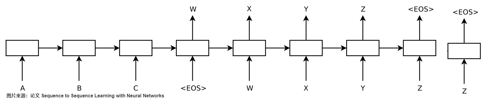
Reused annotated version of Figure 1 from Sutskever, Vinyals, and Le (NIPS 2014). The connected chain reads A B C EOS and predicts W X Y Z EOS. The source EOS marks the handoff in this illustration; it is not the separate target BOS convention used in our prototype. The detached Z -> EOS cell at the far right repeats the last step, rather than extending the connected chain. It does not depict attention or teacher-forcing parallelism.

The figure also exposes why source and target lengths need not match. There is no positionwise assertion $x_i\leftrightarrow y_i$. The decoder keeps applying the next-token factor until EOS.

0x01F The Minimal Runtime Trace

The two loops below implement the same separation. The source loop builds a summary once. The target loop reuses that summary while its own state and previous token change. Notice which object actually becomes an argument to decoder.step:

def fixed_context_generate(source_ids, encoder, decoder, bos_id, eos_id):
    h = encoder.initial_state(batch=source_ids.shape[0])
    encoder_states = []

    for source_column in range(source_ids.shape[1]):
        h = encoder.step(source_ids[:, source_column], h)
        encoder_states.append(h)

    # Prototype contract: only one summary crosses into the decoder.
    context = encoder.project_context(encoder_states[-1])
    state = decoder.initial_state(context)
    previous = full_batch(bos_id)
    output = []

    while not all_finished(output, eos_id):
        state, logits = decoder.step(previous, state, context)
        previous = select_next_token(logits)
        output.append(previous)

    return stack(output, axis=1)

The pseudocode deliberately retains encoder_states while computing the encoder and then passes only context to decoder.step. A framework may keep the state buffer allocated, but allocation is not addressability: if $H$ is not an argument to the decoder read path, the decoder cannot select H[:, j, :] at target step $t$.

This sketch assumes unpadded source rows. For a padded batch, the encoder must respect each source length instead of exporting a state obtained by blindly stepping through padding. A runtime must also track completed rows, stop their output at EOS, and impose a maximum generation length. Those controls complete the loop operationally; none gives the decoder a new way to read an earlier source row.

The same probability factors could be implemented by other architectures. A fixed-input multilayer perceptron can even model a padded finite maximum length. The objection is not that dense layers are mathematically incapable; it is that a monolithic fixed-size mapping does not provide the recurrent weight sharing, variable-length control flow, or source-row retrieval contract being studied here. Transformer blocks still contain dense feed-forward networks; this section is about the whole sequence interface, not a ban on fully connected computation.

0x02 Fixed Context Is An Interface Bottleneck

The model we have just built can assign probabilities, learn from paired sequences, and generate outputs of different lengths. Why change it? Return to the report: producing the translated subject, its assessment, and the committee’s decision may require different details from different source positions. Yet every target step must recover its source evidence from the same summary, constructed before those individual predictions begin.

This motivates the change proposed by Bahdanau, Cho, and Bengio: let the model construct a different source read for each target prediction. To understand what that changes, we first need a precise account of the limitation. It is not simply that “a short vector cannot contain a long sentence”:

A fixed-context decoder has one learned source summary and no direct, target-step-specific operation for addressing the source rows that produced it.

This statement follows from the decoder function signature. It does not require an information-capacity theorem. We can inspect what the decoder receives before making any claim about how well a trained instance will perform.

0x02A What Crosses The Boundary

The next diagram makes the two kinds of state visible at once. Follow the lower source chain into $c$, then follow the dotted connections from $c$ to the upper decoder. The decoder advances through its own states, but each dotted connection supplies the same source-side object.

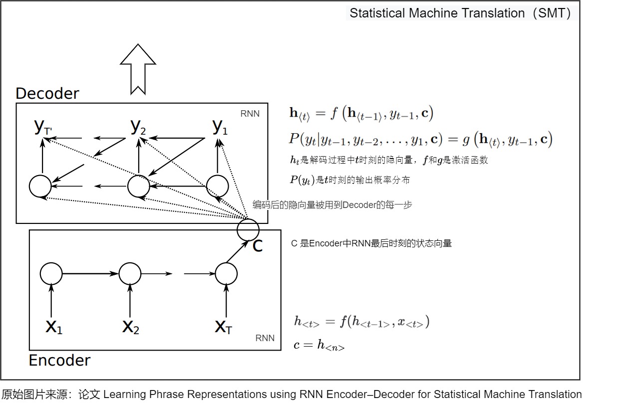
Annotated encoder-decoder based on Cho et al. (EMNLP 2014), not a facsimile of the paper’s full system. Source time runs left to right below; target time runs right to left above, from $y_1$ toward $y_T$. The decoder’s changing state is labeled $h$ in this figure and $s_t$ in our equations. The Chinese annotations identify $c$ as the final encoder state reused at every decoder step. The outer SMT box recalls that the reported neural phrase model was used as a feature in a larger log-linear translation system, not as the whole translation service.

For the final-state prototype,

$$X\longrightarrow H=(h_1,\ldots,h_{T_x}) \longrightarrow c=h_{T_x} \longrightarrow (s_1,\ldots,s_{T_y}).$$

The decoder may carry information forward through $s_t$, but its source-side input remains $c$. The recurrent computation used all earlier source inputs to construct $h_{T_x}$; those inputs are not ignored. What is absent is an operation that exposes a chosen source row $h_j$ to the decoder after the summary has been formed.

Several variants preserve this boundary:

Variant	What changes	What remains fixed
final hidden state	$c=h_{T_x}$	one decoder-visible source vector
projected final state	$c=W_ch_{T_x}+b_c$	one source vector, now with chosen width
final hidden and cell states	several recurrent state tensors initialize the decoder	a source-length-independent state tuple
bidirectional endpoints	$c$ joins final forward/backward summaries	no target-step source-row selection
mean/max/learned pooling	$c=\phi(H)$ uses every row directly during encoding	pooling occurs before the target query is known
source reversal	changes optimization path lengths	does not create an addressable source memory

Sutskever et al. reported that source reversal introduced shorter source-target dependencies and made optimization easier in their experiment. That is a useful alternative design choice. It changes the route by which evidence reaches the final state; it does not change how many source objects cross the encoder-decoder boundary.

0x02B Deriving The Bottleneck From The Function Signature

We can make this limitation independent of a particular drawing. Omit the batch axis for one example and write the source reduction as

$$c=\phi(H), \qquad \phi:\mathbb{R}^{T_x\times d_h}\rightarrow\mathbb{R}^{d_c}.$$

The target distribution we would like to learn is approximated using this summary:

$$p_*(y_t\mid y_{<t},X) \approx p_\theta(y_t\mid y_{<t},c).$$

As above, $p_*$ names the desired distribution and $p_\theta$ the learned model. Within this model, source dependence passes exactly through $c$. For a fixed $c$, two runtime facts follow:

1. the decoder receives the same source-side tensor shape at every target step;
2. the decoder API has no source-row index $j$ and no $H$ argument from which a target-dependent row can be retrieved.

If two source sequences happen to produce the same numerical $c$, this decoder must assign them the same next-token distribution for the same target prefix. That statement is exact for the model graph. It does not prove that a finite-dimensional real vector can never encode an arbitrarily long discrete sequence: such a theorem would require assumptions about precision, continuity, robustness, and the encoder family. Real systems do have finite precision and finite learned capacity, but fixed width alone is not the proof.

The practical pressure instead has four parts:

Pressure	Fixed-context consequence
early commitment	$\phi$ must decide what to retain before the target step asks for evidence
shared source view	all target steps start from the same source summary
long computation path	early source evidence reaches late target steps through encoder and decoder recurrence
hidden alignment	any source-target correspondence must be encoded implicitly inside $c$ and recurrent state

Widening $d_c$ can improve capacity. Better recurrent gates can improve the path. Source reversal can shorten selected dependencies. None gives the decoder a target-conditioned source-row read.

The common short-versus-long-sentence intuition is useful, but it is an engineering pressure rather than a proof. Compare:

short source:  I love you
long source:   The committee that reviewed the report yesterday rejected
               the proposal because it lacked evidence.

The longer source asks one learned state to preserve more entities, clauses, relations, temporal cues, and references. The exact failure point depends on the model, precision, data, and training; source length alone does not prove that a fact has vanished. What remains exact is that the decoder has no direct way to revisit the row where a fact entered.

For example, widening the summary and exposing the source rows are two different interventions to compare. The first gives the encoder more space for its advance summary; the second lets later predictions decide where to read. A measured improvement from one would not establish that the other is unnecessary for every task.

0x02C Addressability Changes Cardinality, Not Context Width Alone

Instead of asking the encoder to finish selecting all source evidence in advance, retain its per-position states. These are often called annotations: learned vectors associated with source positions, not labels added by a human. Collect them as a memory:

$$H=[h_1;\ldots;h_{T_x}] \in\mathbb{R}^{T_x\times d_h}.$$

At target step $t$, a reader uses the currently available target state $q_t$ as a query. The query expresses what this step needs in numerical form; it is not a literal question in natural language. The reader assigns a weight to each source row and combines the rows into a step-specific context:

$$\alpha_t=\operatorname{ReadWeights}(q_t,H), \qquad c_t=\sum_{j=1}^{T_x}\alpha_{t,j}h_j.$$

The sum runs over source positions, leaving one vector for the current target step. If the next query changes the weights, the same stored rows can produce a different context without re-encoding the source. We have not yet specified how to learn useful weights. Section 0x04 derives the score functions, normalization, Bahdanau/Luong state timing, and global versus local candidate sets. Here ReadWeights names that still-to-be-defined operation. The shape change is already visible:

fixed context:
    source interface c        [B, d_c]
    number of source rows directly addressable by decoder = 0

addressable annotations:
    source interface H        [B, T_x, d_h]
    read weights alpha_t      [B, T_x]
    target-specific read c_t  [B, d_h]

Both $c$ and $c_t$ may have fixed width. The change is not necessarily a wider final context or a guarantee of better predictions. The source instead keeps $T_x$ addressable rows, and the decoder can postpone source selection until a target query exists. Compression still happens inside each $h_j$ and inside the weighted read $c_t$; it happens later and conditionally.

Compare the paths in the diagram below. On the fixed-context side, the source row axis ends before decoding. On the addressable side, each target step can reach the retained rows through a different weighted read. The result of a read still has a fixed number of channels; what changed is when and how source information was selected.

Reconstructed interface diagram. Its three displayed target steps are the content-word predictions chat, noir, and dort, after the article le. They illustrate reading noun, modifier, and predicate evidence in a different order from the source. The colored routes are hypothetical, not learned measurements or one-to-one linguistic alignments. The arithmetic example below uses separate supplied weights to test the matrix operation.

0x02D One Source, Three Target Questions

Make the diagram’s example explicit with a reordered toy translation. Words stand in for tokens, and each row label identifies a source position rather than claiming that its vector stores only that word:

source rows:  h_1=the   h_2=black   h_3=cat   h_4=sleeps
target:       le        chat        noir      dort

After the article le, the three content-word predictions ask for the noun, its modifier, and the predicate. In particular, chat precedes noir, while black precedes cat in the source. Alignment need not be one-to-one, and function words may use distributed evidence, but the example makes the source-access difference concrete:

Target step	Evidence the step may need	Fixed-context decoder can access directly	Addressable decoder can access directly
le	article/gender and target grammar	target prefix, state $s_t$, shared $c$	target prefix, state/query, all rows of $H$
chat	source concept at $h_3$	no handle for row 3; evidence may only survive inside $c$	can assign a large read weight to row 3
noir	modifier at $h_2$, despite target reorder	no handle for row 2	can construct a different read emphasizing row 2
dort	predicate at $h_4$	no handle for row 4	can emphasize row 4 or a multi-row phrase

In this table, unavailable means unavailable as a directly addressable runtime object. It does not mean that $c$ contains zero information about the word. A decoder can use information encoded in a summary without having a separate operation that retrieves the original row.

0x02E A Tensor-Level Synthetic Trace

We can check the weighted read without training a translator. Let $B=1$, $T_x=4$, and $d_h=3$: one example, four source positions, and three channels per position. Suppose an encoder exposes the following synthetic annotations:

The listing displays the four rows of the only batch item; the shape labels retain the leading batch axis. The single-vector listings below similarly show the contents of the one batch row, not a change to the batched API.

H [1, 4, 3] =
[
  [0.8, 0.1, 0.0],  # h_1
  [0.1, 0.9, 0.1],  # h_2
  [0.0, 0.2, 0.8],  # h_3
  [0.4, 0.5, 0.6],  # h_4, final recurrent state
]

The final-state fixed prototype exports

c = H[:, -1, :] = [0.4, 0.5, 0.6]   shape [1, 3]

decoder source input at t=1: c
decoder source input at t=2: c
decoder source input at t=3: c

The earlier rows influenced $h_4$ through recurrence, but the decoder cannot request H[:, 1, :] or H[:, 2, :]. In an addressable interface, use three supplied routing rows only to test the contraction:

alpha_1 = [0.80, 0.10, 0.05, 0.05] -> c_1 = [0.670, 0.205, 0.080]
alpha_2 = [0.05, 0.80, 0.10, 0.05] -> c_2 = [0.140, 0.770, 0.190]
alpha_3 = [0.05, 0.05, 0.80, 0.10] -> c_3 = [0.085, 0.260, 0.705]

Each row sums to one and each output is a convex mixture of the same $H$. The numbers prove only the tensor contract alpha_t @ H -> c_t; they do not prove that a trained model would learn these weights or that the weights explain its prediction.

For the first read, the first channel is 0.80*0.8 + 0.10*0.1 + 0.05*0.0 + 0.05*0.4 = 0.670. The same four weights combine the second and third channels to obtain 0.205 and 0.080. Only the weights change for the next read. These three routing rows emphasize source rows 1, 2, and 3 respectively; they are not the diagram’s hypothetical French alignment, which emphasizes rows 3, 2, and 4.

0x02F Code-Level Interface Contrast

The difference now fits in two return values and one read operation. One encoder wrapper exports a summary; the other exports the full source-row axis. The read contracts that axis only after receiving the current query:

def fixed_source_interface(source_ids):
    H = recurrent_encoder(source_ids)       # [B, T_x, d_h]
    c = project(H[:, -1, :])                # [B, d_c]
    return c                                # H is not a decoder input


def addressable_source_interface(source_ids):
    H = contextual_encoder(source_ids)      # [B, T_x, d_h]
    return H                                # row axis survives the boundary


def addressable_read(query_t, H):
    alpha_t = read_weights(query_t, H)      # [B, T_x], derived in Section 0x04
    assert allclose(alpha_t.sum(-1), 1.0)
    c_t = einsum("bt,btd->bd", alpha_t, H)
    return c_t                              # [B, d_h]

The critical assertion is not merely c_t.shape == c.shape. It is that addressable_read receives the source-row axis and the current query, whereas fixed_source_interface removes that axis before decoding. This distinction will also matter when we separate keys used for addressing from values used for the returned content.

There is a resource consequence as well. Retaining the row axis exposes more state to the decoder, and forming each dense read requires work over those rows. Whether the added access is worthwhile depends on the task, learned behavior, and execution cost. Attention introduces an option we can train and evaluate, not a free replacement for every fixed-size summary.

0x02G What The Bottleneck Claim Does And Does Not Establish

The primary papers require a nuanced reading. Bahdanau et al. conjecture that fixed-length encoding is a performance bottleneck and report stronger behavior from soft alignment in their setting. Sutskever et al. report that their LSTM did not have difficulty on long sentences in their evaluated English-to-French task. These are not logically incompatible claims: a useful fixed-vector model can perform well while its source interface remains less selective than an addressable memory.

Claim	What the evidence establishes
the basic decoder receives one source summary	the cited Cho/Sutskever prototypes expose this interface
Bahdanau et al. motivate soft search as relief from that bottleneck	the paper makes this argument and evaluates an addressable-source model
fixed width alone proves unavoidable information loss	not established without additional assumptions
longer inputs often increase optimization and retention pressure	plausible and empirically testable, not universal from shape alone
addressable source rows guarantee correct alignment or faithfulness	false; access is available, but learning and explanation remain separate

Attention therefore changes a concrete software and tensor boundary. It does not abolish compression, guarantee long-context quality, or make attention weights a causal explanation.

0x02H What Changes When Source Rows Remain Available

The distinction can now be stated at four levels:

1. $P(Y\mid X)$ is factorized by the conditional chain rule, independently of the neural architecture used to parameterize each factor.
2. a fixed-context recurrent prototype maps $[B,T_x,d_h]$ source state to a source-length-independent $[B,d_c]$ decoder interface;
3. the deeper bottleneck is the absence of target-conditioned source-row access, not a theorem that a fixed-width vector contains no source evidence;
4. retaining $H$ makes a row axis available to a later read mechanism.

Exposing the source rows does not yet specify how to construct them or how to choose a useful read. We next examine recurrent state construction, then derive the attention read and compare it with convolutional paths through a sequence.

0x03 Recurrence: State, Time, And Gradient Paths

The fixed-context interface in 0x02 says what crosses from encoder to decoder. Recurrence answers a different question: how is one stream state constructed from an ordered sequence? A recurrent model applies one learned transition repeatedly, so parameter count need not grow with sequence length:

$$a_t = W_x x_t + W_h h_{t-1} + b, \qquad h_t = \phi(a_t).$$

For a batch of $B$ sequences, $x_t\in\mathbb{R}^{B\times d_x}$, $h_t\in\mathbb{R}^{B\times d_h}$, $W_x\in\mathbb{R}^{d_h\times d_x}$, and $W_h\in\mathbb{R}^{d_h\times d_h}$. The same $W_x,W_h,b$ are used for every $t$. The displayed recurrence uses column-vector notation for one example; a row-batched implementation computes x_t @ W_x.T + h_prev @ W_h.T + b. Variable length changes the number of transition applications, not the number of recurrent parameter objects.

This architecture has three properties that must not be collapsed into one claim:

Property	Exact contract	What it does not imply
recurrent state	$h_t$ is an explicit function of $h_{t-1}$ and $x_t$	that all useful history is perfectly retained
sequential schedule	$h_t$ cannot be evaluated before $h_{t-1}$ exists	that every operation surrounding the cell is scalar or slow
shared transition	the same parameters are reused across time	that gradients through many uses remain well conditioned

Recurrence is therefore both a useful memory bias and a long dependency chain. That is a trade, not a verdict that recurrent models are obsolete.

0x03A Forward State And Runtime Schedule

The smallest executable trace has one loop-carried tensor:

def recurrent_encode(x, cell, h0):
    # x: [B, T, d_x], h: [B, d_h]
    h = h0
    states = []
    for t in range(x.shape[1]):
        h = cell(x[:, t, :], h)
        states.append(h)
    return stack(states, axis=1), h  # [B,T,d_h], [B,d_h]

states[:, t] cannot be produced before states[:, t-1], even though the matrix operations inside one cell can process all $B$ batch rows and all $d_h$ channels in parallel. “RNNs are sequential” means there is a loop-carried dependency along $T$; it does not mean the cell contains no parallel linear algebra.

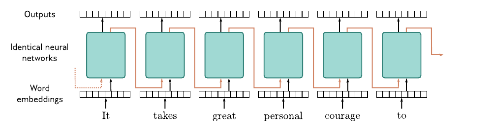
Simon Prince, Understanding Deep Learning, Chapter 12, Figure 12.19 (CC-BY-NC-ND / MIT Press). The repeated orange state edge shows the loop-carried dependency. The drawing does not assert that every RNN has one state tensor, nor that information is necessarily lost at each arrow.

For two positions $k<t$, the forward influence of $x_k$ on $h_t$ crosses $t-k$ recurrent transitions. In a recurrent encoder-decoder without an addressable source memory, a source-to-target route can be longer still:

x_k -> h_k -> ... -> h_Tx -> decoder state_1 -> ... -> decoder state_t -> y_t

This is the communication path. It is related to, but distinct from, the gradient path used to learn the transition.

0x03B Backpropagation Through Time Exposes A Jacobian Product

Let a loss at step $t$ be $E_t(h_t)$. For any earlier state $h_k$, the chain rule gives

$$\frac{\partial E_t}{\partial h_k} = \frac{\partial E_t}{\partial h_t} \frac{\partial h_t}{\partial h_k}, \qquad \frac{\partial h_t}{\partial h_k} = \prod_{j=k+1}^{t} \frac{\partial h_j}{\partial h_{j-1}}.$$

For the tanh cell above,

$$J_j := \frac{\partial h_j}{\partial h_{j-1}} = \operatorname{diag}\!\left(1-h_j^2\right)W_h,$$

so learning a dependency across $t-k$ steps requires transporting an error through $J_tJ_{t-1}\cdots J_{k+1}$. Using any compatible matrix norm,

$$\left\|\frac{\partial h_t}{\partial h_k}\right\| \le \prod_{j=k+1}^{t}\|J_j\|.$$

If every local norm is bounded by $\eta<1$, the upper bound decays as $\eta^{t-k}$. If products repeatedly expand an aligned direction, a long-term component can grow rapidly instead. Pascanu, Mikolov, and Bengio analyze this matrix-product mechanism and separate vanishing long-term components from exploding ones. (Pascanu et al.)

A scalar teaching case makes the exponent visible. If the local derivative is approximately $0.8$ for twenty transitions, its contribution is

$$0.8^{20}\approx 0.01153.$$

If it is approximately $1.1$, the corresponding factor is

$$1.1^{20}\approx 6.7275.$$

These numbers are not an RNN benchmark. Real Jacobians are matrices, their directions change with state, and tanh saturation changes the derivative. The example establishes only why repeated multiplication can create distance- dependent optimization pressure.

0x03C State Capacity, Forward Paths, And Gradient Conditioning Are Different

Three common diagnoses refer to different objects:

Diagnosis	Object under pressure	Observable failure
compressed state	$h_t\in\mathbb{R}^{d_h}$ must summarize a growing prefix	evidence is overwritten, entangled, or hard to recover
long forward path	a distant influence crosses many nonlinear transitions	later state depends only indirectly on early state
ill-conditioned backward path	a product of Jacobians transports the error	long-term gradient components shrink or grow

Increasing $d_h$ may increase representational capacity without shortening the path. Gradient clipping can control an exploding update without recovering a vanished component. A gate can create a better carry path while retaining the same sequential schedule. Attention later changes source-state addressability; it is not merely another clipping rule or a wider hidden state.

Norm clipping from Pascanu et al. is mechanically simple:

g = gradient(loss, parameters)
if norm(g) >= threshold:
    g = threshold * g / norm(g)
optimizer_step(g)

This rescales a large gradient vector while preserving its direction. It is a response to explosion, not a proof that long-range credit assignment is solved, and not a modification of the forward recurrent path.

0x03D GRU: An Explicit Carry-Or-Write Choice

Cho et al. proposed the gated hidden unit used in their RNN Encoder-Decoder. In the paper’s convention,

$$\begin{aligned} r_t &= \sigma(W_r x_t + U_r h_{t-1}),\\ z_t &= \sigma(W_z x_t + U_z h_{t-1}),\\ \widetilde h_t &= \phi\!\left(Wx_t+U(r_t\odot h_{t-1})\right),\\ h_t &= z_t\odot h_{t-1}+(1-z_t)\odot\widetilde h_t. \end{aligned}$$

The reset gate $r_t$ controls how much previous state enters the candidate. The update gate $z_t$ interpolates between carrying the previous state and writing the candidate. Under this convention, $z_t\approx1$ carries and $z_t\approx0$ writes. Some libraries and later descriptions reverse the names of the interpolation coefficients; the executable equation, not the prose label, is the contract. (Cho et al., EMNLP 2014)

For one supplied two-channel state,

h_prev      = [ 0.80, -0.40]
h_candidate = [ 0.20,  0.60]
z           = [ 0.90,  0.25]
h_new       = z*h_prev + (1-z)*h_candidate
            = [ 0.74,  0.35]

Channel 1 mostly carries old state; channel 2 mostly writes the candidate. This is more expressive than replacing every channel with one tanh update, but h_new still cannot be computed before h_prev.

0x03E LSTM: The Paper Lineage Matters

The phrase “the LSTM equations” hides a historical variant boundary. The 1997 LSTM paper introduced a memory cell with constant-error-flow motivation plus learned input and output gates. The adaptive forget gate familiar from modern LSTMs was introduced later for continual streams. (Hochreiter and Schmidhuber, 1997, Gers, Schmidhuber, and Cummins, 2000)

A common modern form is

$$\begin{aligned} i_t &= \sigma(W_i x_t+U_i h_{t-1}+b_i),\\ f_t &= \sigma(W_f x_t+U_f h_{t-1}+b_f),\\ o_t &= \sigma(W_o x_t+U_o h_{t-1}+b_o),\\ g_t &= \tanh(W_g x_t+U_g h_{t-1}+b_g),\\ c_t &= f_t\odot c_{t-1}+i_t\odot g_t,\\ h_t &= o_t\odot\tanh(c_t). \end{aligned}$$

Holding the gate values fixed, the direct derivative along the cell-state path is $\partial c_t/\partial c_{t-1}=\operatorname{diag}(f_t)$. Values of $f_t$ near one can preserve a component; values near zero intentionally reset it. The full derivative also contains indirect paths because gates depend on $h_{t-1}$, so “LSTM has constant gradients” is too strong for the modern cell.

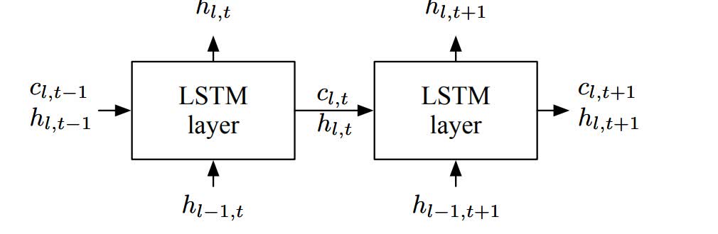
Illustration of a stacked LSTM’s state paths. The figure exposes the two loop-carried tensors $c_{l,t}$ and $h_{l,t}$. It supports “gated memory still recurs”; it does not specify which historical LSTM variant or prove well-conditioned gradients.

0x03F Recurrent Design Choices Change Memory, Not The Time Dependency

Design	What changes	What remains sequential
vanilla RNN	one nonlinear state update	$h_t$ requires $h_{t-1}$
GRU	reset and update gates choose candidate/carry mixtures	$h_t$ requires $h_{t-1}$
modern LSTM	separate cell/hidden paths plus input, forget, and output gates	$(c_t,h_t)$ require $(c_{t-1},h_{t-1})$
bidirectional encoder	one left-to-right and one right-to-left chain	each direction is recurrent; full input must be available
source reversal	changes which source-target relations cross the longest chain	the recurrent transition and serial schedule remain
truncated BPTT	limits the backward unroll used for an update	forward recurrence still carries state across steps if retained
gradient clipping	bounds an oversized gradient norm	forward state and Jacobian-product depth are unchanged

Sutskever et al. reported that reversing source order introduced shorter source-to-target dependencies in their setup and made optimization easier. It did not remove recurrence or make every dependency short. Bidirectionality is appropriate when the complete input is known; it is not a causal streaming decoder. These alternatives show why the correct history is “different contracts for different pressures,” not “RNNs failed and disappeared.”

0x03G A Better State Update Is Not A New Read Interface

LSTM and GRU improve what happens inside the recurrent edge. The fixed-context decoder from 0x02 still receives one source-side object unless the architecture retains and exposes the encoder row sequence. The next section derives the target-conditioned read over those rows. Convolution in 0x05 will change the within-layer schedule and path geometry without, by itself, specifying that read.

0x04 Attention as soft alignment

The fixed-context analysis in 0x02 established the interface pressure: one source vector does not expose separately addressable source rows. Attention changes that interface by computing a target-dependent read from a set of encoder annotations. The original sequence-to-sequence mechanism is therefore the right starting point, before projected queries/keys/values, multi-head layouts, or Transformer self-attention.

This section keeps three contracts separate:

generic attention:
    an already-available query scores a memory and returns one context

Bahdanau et al.:
    previous decoder state -> alignment -> context -> new decoder state

Luong et al.:
    current decoder state -> alignment -> context -> attentional state

The state ordering is part of the algorithm. Replacing every query symbol with s_t hides a circular dependency in the Bahdanau variant.

0x04A Alignment Is Not Position Equality

Translation alignment is not generally source position i -> target position i. Words can reorder, one phrase can map to several words, and function words can appear or disappear. A rough example is

source: The black cat sleeps
target: Le  chat  noir dort

Le   <- The
chat <- cat
noir <- black
dort <- sleeps

Even this list is too rigid for many phrase-level translations. A hard alignment chooses discrete links. A soft alignment assigns continuous coefficients to several source annotations, allowing the model to mix evidence and train the alignment path with ordinary backpropagation.

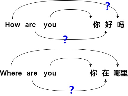
Illustrative bilingual alignment. The Chinese targets are examples of reordered and non-one-to-one translation. The arrows motivate the alignment problem; they are not learned model outputs and do not define a unique gold alignment.

Bahdanau, Cho, and Bengio framed their proposal as automatically soft-searching the source positions relevant to the current target prediction. They described the fixed-length source vector as a conjectured bottleneck and reported qualitatively plausible alignments; those are source claims, not a theorem that every soft alignment is linguistically correct. (Bahdanau et al., ICLR 2015)

0x04B Generic Attention Starts With An Available Query

Let the encoder expose

$$H=[h_1;\ldots;h_{T_x}] \in\mathbb{R}^{B\times T_x\times d_h},$$

and let

$$q_t\in\mathbb{R}^{B\times d_q}$$

be a query that already exists before the read begins. The generic score contract is

$$e_{t,i}=\operatorname{score}(q_t,h_i), \qquad e_t\in\mathbb{R}^{B\times T_x}.$$

t indexes the query/output row; i indexes source memory. The score function must return one scalar per (batch, query, source) pair. At this historical level, the same annotation $h_i$ can participate in both scoring and mixing. Later, separate learned projections will let a source row carry different representations for matching and for the content returned.

Padding is an axis contract, not cleanup after softmax. If $M\in\{0,1\}^{B\times T_x}$ marks valid source rows, use

$$\bar e_{t,i} = \begin{cases} e_{t,i}, & M_i=1,\\ -\infty, & M_i=0. \end{cases}$$

For numerical stability, subtract the largest valid score $m_t=\max_{i:M_i=1}\bar e_{t,i}$ and normalize over the source axis:

$$\alpha_{t,i} = \frac{\exp(\bar e_{t,i}-m_t)} {\sum_{j:M_j=1}\exp(\bar e_{t,j}-m_t)}.$$

Because exponentials are positive,

$$\alpha_{t,i}\ge0, \qquad \sum_{i:M_i=1}\alpha_{t,i}=1.$$

Subtracting $m_t$ changes neither weight: multiplying numerator and denominator by the same $\exp(-m_t)$ cancels. The context is then

$$c_t = \sum_{i=1}^{T_x}\alpha_{t,i}h_i \in\mathbb{R}^{B\times d_h}.$$

The source axis contracts away. One context row remains for each query row. This is the exact cardinality change that the fixed-vector interface lacked.

Transformer System reconstruction. The diagram fixes tensor ownership and the softmax axis. It is a read contract, not a Transformer multi-head block or a claim that the largest coefficient is a causal explanation.

0x04C A Numeric Read Makes The Contraction Auditable

For one batch row, take

$$H= \begin{bmatrix} 1&0\\ 0&2\\ -1&1\\ 2&-1 \end{bmatrix}, \qquad q_t=[1,0.5].$$

Using a dot score only for this synthetic trace gives

scores e_t       = [ 1.0000, 1.0000, -0.5000, 1.5000 ]
stable exponents = exp(e_t - 1.5)
weights alpha_t  = [ 0.258274, 0.258274, 0.057629, 0.425822 ]
sum(alpha_t)     = 1.000000
context c_t      = [ 1.052290, 0.148355 ]

The context is neither the query nor one selected source row. It is a convex mixture of the supplied source rows. This fixture validates the contraction; it is not a trained translation example.

def attention_read(query, memory, valid_mask, score_fn):
    # query [B,d_q], memory [B,T_x,d_h]
    scores = score_fn(query[:, None, :], memory)       # [B,T_x]
    scores = where(valid_mask, scores, -inf)
    scores = scores - max(scores, axis=1, keepdims=True)
    weights = softmax(scores, axis=1)                  # source axis
    context = einsum("bt,btd->bd", weights, memory)   # [B,d_h]

    assert_allclose(weights[~valid_mask], 0.0)
    assert_allclose(weights.sum(axis=1), 1.0)
    return context, weights

The all-masked case must be rejected or handled by an explicit policy; it has no valid probability denominator.

0x04D Why The Alignment Network Can Learn

Soft attention replaces a discrete source choice with differentiable score, normalization, and weighted-sum operations. The softmax derivative is

$$\frac{\partial\alpha_{t,j}}{\partial e_{t,i}} = \alpha_{t,j}(\mathbf{1}_{i=j}-\alpha_{t,i}).$$

Holding the source annotations fixed and differentiating $c_t=\sum_j\alpha_{t,j}h_j$ gives

$$\frac{\partial c_t}{\partial e_{t,i}} = \alpha_{t,i}(h_i-c_t).$$

The derivation follows by substituting the softmax Jacobian:

$$\sum_j h_j\alpha_{t,j}(\mathbf{1}_{i=j}-\alpha_{t,i}) = \alpha_{t,i}h_i-\alpha_{t,i}\sum_j\alpha_{t,j}h_j.$$

Thus a score receives signal according to how its source annotation differs from the current mixture. Gradients also flow into the annotations and the query through the score function. This is what permits joint alignment and translation training. It does not mean softmax learns a unique alignment or that every coefficient is independently identifiable.

0x04E Bahdanau: Context Before The New Decoder State

The Bahdanau paper does not score with an already-computed $s_t$. Its encoder is bidirectional and forms one annotation per source position:

$$h_j=[\overrightarrow h_j;\overleftarrow h_j].$$

At target step $t$, the previous decoder state is available. The paper’s feed-forward additive alignment model is

$$e_{t,j} = v_a^\top\tanh(W_a s_{t-1}+U_a h_j),$$

followed by

$$\alpha_{t,j} = \frac{\exp(e_{t,j})}{\sum_{k=1}^{T_x}\exp(e_{t,k})}, \qquad c_t=\sum_{j=1}^{T_x}\alpha_{t,j}h_j.$$

Only after $c_t$ exists is the new decoder state computed:

$$s_t=f(s_{t-1},E_y[y_{t-1}],c_t),$$

and the output distribution is formed from the previous token, new state, and context:

$$p(y_t\mid y_{<t},x)=g(E_y[y_{t-1}],s_t,c_t).$$

The state order is therefore

s_(t-1) + source annotations
    -> e_t -> softmax over source j -> c_t
    -> decoder update with y_(t-1) -> s_t
    -> target distribution for y_t

There is no circular use of $s_t$ to create the context needed to compute $s_t$.

def bahdanau_step(prev_token, prev_state, source, source_mask):
    # source [B,T_x,d_h], prev_state [B,d_s]
    joint = Wa(prev_state)[:, None, :] + Ua(source)     # [B,T_x,d_a]
    scores = einsum("bta,a->bt", tanh(joint), va)      # [B,T_x]
    context, alpha = normalized_source_read(scores, source, source_mask)
    state = decoder_cell(embed(prev_token), prev_state, context)
    logits = output_head(embed(prev_token), state, context)
    return logits, state, alpha

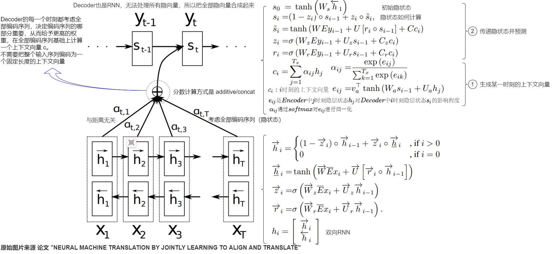
Annotated reconstruction of Bahdanau et al.’s Figure 1 and appendix equations. The Chinese notes identify (1) context construction and (2) recurrent-state propagation. The operative order is $s_{t-1}\rightarrow\alpha_t\rightarrow c_t\rightarrow s_t$; the dense annotation is explained by the English state trace in the comparison below.

0x04F Luong: Current Decoder State Before Context

Luong, Pham, and Manning use a different ordering. A stacked LSTM first produces the current top-layer target state $h_t$. Global attention then scores that state against every top-layer source state $\bar h_s$:

$$a_t(s) = \frac{\exp(\operatorname{score}(h_t,\bar h_s))} {\sum_{s'=1}^{T_x}\exp(\operatorname{score}(h_t,\bar h_{s'}))}, \qquad c_t=\sum_s a_t(s)\bar h_s.$$

The context and current target state are combined into a separate attentional state,

$$\widetilde h_t=\tanh(W_c[c_t;h_t]),$$

and the output distribution is

$$p(y_t\mid y_{<t},x)=\operatorname{softmax}(W_s\widetilde h_t).$$

The Luong path is

y_(t-1) + recurrent state_(t-1)
    -> current top decoder state h_t
    -> a_t -> c_t -> attentional state h_tilde
    -> target distribution for y_t

That is not merely Bahdanau attention with another score function. The context enters at a different point in the recurrent/output graph. (Luong et al., EMNLP 2015)

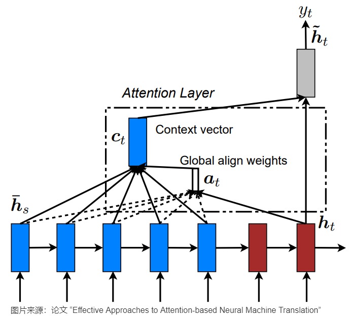
Luong et al., Figure 2. The current decoder state $h_t$ produces global alignment weights $a_t$; the context $c_t$ and $h_t$ then produce $\widetilde h_t$. The Chinese footer only identifies the paper source.

Transformer System reconstruction from the two primary papers. The figure compares data dependencies, not measured quality or runtime.

0x04G Score Function And Memory Window Are Independent Choices

The query timing, score family, and visible source set are separate axes. Luong et al. tested several functions; their printed equations should not be silently replaced by later conventions.

Paper choice	Score	Shape/design contract
Bahdanau additive	$v_a^\top\tanh(W_a q+U_a h_i)$	projections permit $d_q\ne d_h$; hidden alignment width $d_a$ is explicit
Luong dot	$h_t^\top\bar h_s$	target/source state widths must match
Luong general	$h_t^\top W_a\bar h_s$	learned bilinear map; can reconcile representation geometry
Luong concat, Eq. 8	$W_a[h_t;\bar h_s]$	the paper prints a learned scalar row over the concatenation
Luong location, Eq. 9	$a_t=\operatorname{softmax}(W_a h_t)$	no source content enters the score; output length must be provisioned

The nonlinear expression often called “concat attention” in later summaries, $v^\top\tanh(W[q;h])$, is structurally closer to additive attention. It should not be attributed to Luong Eq. 8 without qualification. Scaled dot-product, projected Q/K/V roles, and their matrix implementation belong to M3.1.

0x04H Global, Local-m, Local-p, And Input Feeding

Luong’s global model scores all $T_x$ source states for each target query. Its alignment row has variable length $T_x$. The local model first defines a center $p_t$ and attends only to integer source positions in $[p_t-D,p_t+D]$ that remain inside the sentence.

The monotonic variant fixes

$$p_t=t \qquad\text{(local-m)},$$

encoding a rough monotonic-alignment prior. The predictive variant learns

$$p_t = T_x\,\sigma\!\left(v_p^\top\tanh(W_p h_t)\right) \qquad\text{(local-p)},$$

so $p_t\in[0,T_x]$. For a source position $s$ in the selected window, the paper multiplies the content alignment by a Gaussian envelope:

$$a_t(s) = \operatorname{align}(h_t,\bar h_s) \exp\!\left(-\frac{(s-p_t)^2}{2\sigma^2}\right), \qquad \sigma=\frac{D}{2}.$$

The paper’s Eq. 11 does not print a second normalization after this multiplication. Therefore the generic “weights sum to one” proof applies to the align softmax row, not automatically to the Gaussian-modulated final local-p coefficients. An implementation that renormalizes after applying the envelope is a variant and should say so.

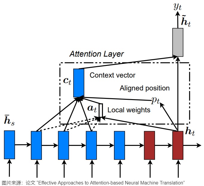
Luong et al., Figure 3. The model predicts an aligned position $p_t$, restricts the source window, computes local weights, and then forms $c_t$. The source figure does not show the local-m/local-p formula difference by itself.

Luong et al. also introduce input feeding. The previous attentional state is concatenated with the next target embedding before the recurrent update:

decoder input at t+1 = [ E_y[y_t] ; h_tilde_t ]

This lets later decisions depend on prior attention choices and creates a horizontal alignment-history path. It is a learned history signal, not a hard guarantee that every source word is covered exactly once.

Choice	Source rows scored	Added inductive bias	Main cost/boundary
global content	$T_x$	none beyond score function	linear source scan per target query
location	provisioned output positions	query-only position pattern	no source-content comparison
local-m	at most $2D+1$	monotonic center $p_t=t$	poor fit for strong reordering
local-p	at most $2D+1$	learned center plus Gaussian locality	window gather and center predictor
input feeding	unchanged	prior attentional state enters next step	stronger target-time dependency

This is a paper-level alternative map, not a claim that local attention is always faster on modern hardware. Gather overhead, sequence lengths, batching, and kernels belong to M4.

0x04I Tensor Schedule, Training, And Runtime Integration

For one global cross-attention step with $B=2$, $T_x=5$, $d_h=8$, and an alignment width $d_a=6$:

Object	Shape	Owner/lifetime
source annotations $H$	$[2,5,8]$	encoder output, reusable across target steps
available query	Bahdanau $s_{t-1}$ or Luong $h_t$	one decoder step
projected additive joint rows	$[2,5,6]$	temporary score state
scores / alignment row	$[2,5]$	one scalar per source row
source mask	$[2,5]$	request/example metadata
context $c_t$	$[2,8]$	target-step-owned weighted source state

The source-axis work can be batched. The original decoder time axis cannot:

Bahdanau: s_t depends on c_t, which depends on s_(t-1)
Luong:    h_t depends on h_(t-1); optional input feeding also uses h_tilde_(t-1)

Teacher forcing supplies known previous target tokens during training, but it does not remove those recurrent state dependencies. At inference, the encoder annotations are computed once, then each target step scores either all source rows or one local window. This is cross-attention attached to a recurrent decoder, not the row-parallel Transformer decoder training contract.

The paper experiments also differ beyond attention formulas:

Source-reported system	Training/model context	Why it matters here
Bahdanau RNNsearch	bidirectional source RNN, recurrent decoder, 30k vocabularies, minibatch 80, Adadelta; length-30 and length-50 training variants	additive attention was trained as part of a complete recurrent NMT system
Luong models	four-layer 1000-cell stacked LSTMs, 1000-dimensional embeddings, minibatch 128, SGD schedule, gradient clipping at norm 5, optional dropout and input feeding	dot/general/global/local results are coupled to a different recurrent and optimization contract

These values are source-reported historical context, not recommended modern hyperparameters and not a controlled head-to-head reproduction.

0x04J Alignment Is Visible; Explanation Is A Stronger Claim

For a generated target sequence, stacking alignment rows creates a matrix with target positions on one axis and source positions on the other. Bahdanau et al. used such matrices to inspect non-monotonic phrase alignments. Luong et al. also evaluated one-to-one links extracted from forced decoding with alignment error rate. This supports a historical claim: the coefficients can be visualized as soft source-target alignment inside these models.

It does not establish that an attention map is a faithful causal explanation of a prediction. The coefficients are internal routing values; later computation, correlated representations, alternative weight patterns, and intervention behavior all matter. Jain and Wallace found that standard attention weights were often weakly related to gradient feature-importance measures and that very different distributions could yield similar predictions. (Jain and Wallace, NAACL 2019)

valid statement:
    alpha records how this attention module mixed its supplied value rows

stronger statement requiring separate evidence:
    alpha explains why the complete model produced this output

The second statement does not follow from the first.

0x04K From A Source Read To Sequence Interaction

The durable mechanism is now precise:

available query
    -> score addressable source rows
    -> normalize over the visible source axis
    -> contract source rows into one query-owned context

Bahdanau and Luong implement that read inside different recurrent state graphs. Neither removes encoder/decoder recurrence, and neither is Transformer multi-head self-attention. Attention changed the source read interface before the Transformer made it a principal within-stream interaction operation. To understand that further change, we must also examine how a model updates many positions together and how it trains a deep stack.

0x05 Convolution: Parallel Rows, Depth-Bounded Context

Convolution changes the sequence schedule without requiring a recurrent state. Within one layer, every output row reads a window from the previous layer, so all output positions whose inputs are available can be evaluated together. The trade is that the connectivity pattern is chosen by kernel geometry before the input content is known.

0x05A One-Dimensional Convolution As A Tensor Contract

Let $X^{(\ell-1)}\in\mathbb{R}^{B\times T\times d}$ be the input to layer $\ell$. For a width-$k$ convolution, gather one local window per output row:

$$U_i^{(\ell)} = \operatorname{concat} \left( X_{i+o_1}^{(\ell-1)},\ldots,X_{i+o_k}^{(\ell-1)} \right) \in\mathbb{R}^{B\times kd}.$$

The offsets $o_1,\ldots,o_k$ encode the visibility contract. A non-causal encoder can use centered offsets. An autoregressive decoder must use only current/earlier target inputs, with a shift chosen so the row predicting $y_{i+1}$ cannot read $y_{i+1}$.

One shared kernel then produces

$$Y_i^{(\ell)} = U_i^{(\ell)}W_\ell^\top+b_\ell.$$

All $T$ windows can be packed as $U^{(\ell)}\in\mathbb{R}^{B\times T\times kd}$ and multiplied in one batched operation. Parameter sharing means the same $W_\ell$ is applied at every position; it does not mean every position receives the same activation.

def conv1d_rows(x, offsets, weight, bias):
    # x: [B,T,d], windows: [B,T,k,d]
    windows = gather_windows(x, offsets=offsets, pad_value=0)
    packed = windows.reshape(B, T, len(offsets) * d)
    return packed @ weight.T + bias

The loop over positions is absent from the dependency graph of one layer. The loop over layers remains because layer $\ell$ consumes layer $\ell-1$.

0x05B Deriving The Receptive Field

Assume stride one and no pooling. Let $R_\ell$ be the span, measured in original input coordinates, that can influence one output after layer $\ell$, with $R_0=1$. A width-$k_\ell$ kernel at dilation $d_\ell$ samples positions across an additional span of $(k_\ell-1)d_\ell$. Therefore

$$R_\ell = R_{\ell-1}+(k_\ell-1)d_\ell,$$

and after $L$ layers,

$$R_L = 1+\sum_{\ell=1}^{L}(k_\ell-1)d_\ell.$$

For contiguous convolutions, $d_\ell=1$. If every layer has width $k$,

$$R_L=1+L(k-1).$$

This reproduces the ConvS2S paper’s example: six blocks of width five yield

$$R_6=1+6(5-1)=25$$

input positions. It also shows why “a width-five kernel sees the whole sentence” is false: width and depth jointly determine the maximum field.

For exponentially increasing dilations $d_\ell=2^{\ell-1}$,

$$R_L = 1+(k-1)\sum_{\ell=1}^{L}2^{\ell-1} = 1+(k-1)(2^L-1).$$

With $k=2$ and dilations $1,2,4,8$, four layers cover $R_4=16$ positions. WaveNet used repeated dilation cycles such as $1,2,4,\ldots,512$ to obtain a large causal receptive field without a 1024-wide dense kernel. (WaveNet)

In plain notation:

contiguous: R_L = 1 + L * (k - 1)
dilated:    R_L = 1 + sum_l (k_l - 1) * dilation_l
doubling:   R_L = 1 + (k - 1) * (2^L - 1)

The formula tracks the outer span of the architectural field. When the sampled supports overlap, every position in that span is reachable; arbitrary dilation schedules can instead leave holes. Neither span nor coverage proves that training uses every reachable position effectively.

0x05C Depth Replaces Time As The Local Communication Route

For a causal contiguous stack, each width-$k$ layer can extend the furthest backward dependency by at most $k-1$ positions. Connecting a row to evidence $\Delta$ positions earlier therefore requires at least

$$L_{\text{contiguous}} \ge \left\lceil\frac{\Delta}{k-1}\right\rceil$$

layers. With $k=5$ and $\Delta=24$, the lower bound is six layers, consistent with the 25-position field above. With a doubling dilation schedule, the coverage condition is

$$(k-1)(2^L-1)\ge\Delta,$$

or

$$L_{\text{dilated}} \ge \left\lceil \log_2\!\left(1+\frac{\Delta}{k-1}\right) \right\rceil.$$

This comparison is about dependency-graph depth under the stated padding, stride, and dilation assumptions. It is not a latency benchmark. Larger kernels and dilation alter memory access, arithmetic, utilization, and optimization behavior, which M4 treats quantitatively.

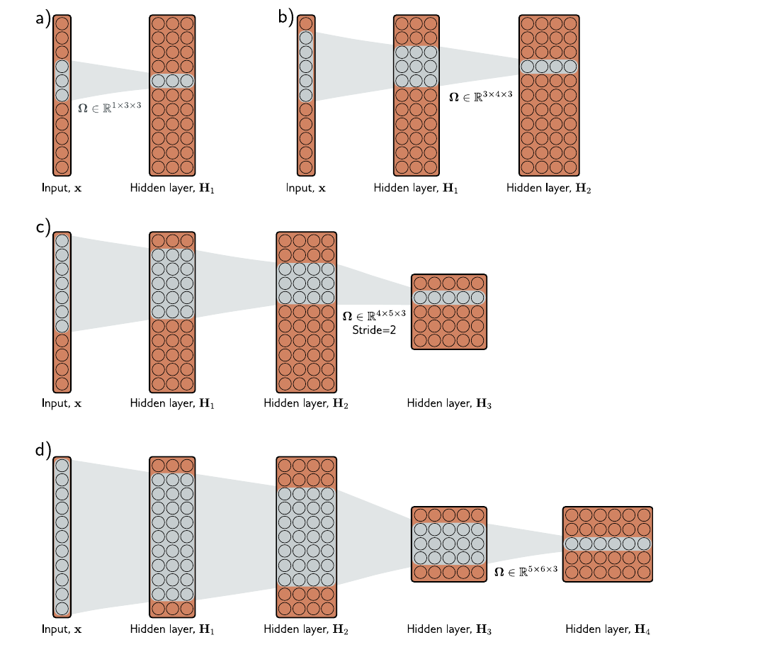
Simon Prince, Understanding Deep Learning, Chapter 10, Figure 10.6 (CC-BY-NC-ND / MIT Press). The panels show one-dimensional convolutions, channels, and receptive-field growth; some include stride. The derivation above assumes stride one, so its span formula must not be applied unchanged to the strided cases.

0x05D Parallel Training Does Not Remove Autoregressive Generation

For a teacher-forced target $y_{0:T-1}$, every shifted target input is known. A causal convolution can therefore evaluate all target rows in parallel while its mask/padding prevents future leakage:

training row i input: known prefix tokens ending at y_i
training row i output: distribution for y_(i+1)

During generation, $y_{i+1}$ is unknown until the model selects it. Removing recurrent hidden-state dependence permits row-parallel training, but the autoregressive factorization still exposes one new token decision at a time. This is the same task/architecture distinction derived in 0x01. Efficient incremental convolution can retain recent layer inputs instead of recomputing the full prefix, but cache mechanics belong to M5.

0x05E ConvS2S Was Convolution Plus Several Other Design Choices

Gehring et al.’s ConvS2S is the important paper contract, not a generic slogan that “CNNs replaced RNNs.” It used:

1. word embeddings plus learned absolute position embeddings;
2. stacked one-dimensional encoder and causal decoder convolutions;
3. gated linear units (GLUs);
4. residual connections around convolutional blocks;
5. a separate encoder-decoder attention module in every decoder layer.

For a decoder window flattened to $u_i^{(\ell)}\in\mathbb{R}^{kd}$, the paper’s convolution produces twice the channel width and splits it:

$$[A_i^{(\ell)},B_i^{(\ell)}] = W_\ell u_i^{(\ell)}+b_\ell, \qquad A_i^{(\ell)},B_i^{(\ell)}\in\mathbb{R}^{d}.$$

The GLU and residual update are

$$v_i^{(\ell)} = A_i^{(\ell)}\odot\sigma(B_i^{(\ell)}), \qquad h_i^{(\ell)} = h_i^{(\ell-1)}+v_i^{(\ell)}.$$

The $B$ half controls which transformed $A$ channels pass. This is a gate inside a depth-parallel convolutional block, not a recurrent state gate.

def convs2s_block(h, offsets, W, b):
    # h [B,T,d] -> packed windows [B,T,k*d]
    u = gather_windows(h, offsets).reshape(B, T, k * d)
    a, gate_logits = split((u @ W.T) + b, 2, axis=-1)
    update = a * sigmoid(gate_logits)
    return h + update

The paper then computes a source context separately at every decoder layer. The attention result is added to that layer’s decoder state and can influence the next layer’s attention. “Entirely convolutional” means recurrence was removed from the encoder and decoder state transitions; it does not mean the architecture omitted attention. (Gehring et al., ICML 2017)

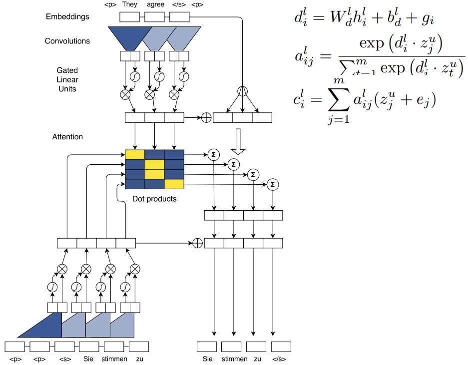
Gehring et al., Figure 1. The upper decoder path shows convolution, GLU, and residual addition; the lower path shows the convolutional encoder. The central matrix is batched cross-attention over known target rows during training. This figure demonstrates per-layer attention, not a purely local encoder-decoder.

0x05F A Paper-Level Shape Trace

For $B=2$, $T=7$, $d=4$, and $k=3$:

Object	Shape	Role
previous layer $h^{(\ell-1)}$	$[2,7,4]$	one row per sequence position
gathered windows	$[2,7,3,4]$	three local rows per output row
flattened windows	$[2,7,12]$	kernel input axis
$W_\ell$	$[8,12]$	produces $2d$ GLU channels
pre-GLU output	$[2,7,8]$	split into $A,B$
gated update	$[2,7,4]$	$A\odot\sigma(B)$
residual output	$[2,7,4]$	same row/channel ownership as input

The residual addition is legal because the update returns to width $d$. A projection is required if the block changes width. 0x06 derives that addition. The next section explains why that shortcut also changes the backward path through a deep stack.

0x05G Alternatives Change The Field-Cost Trade

Choice	Gains	Costs or boundary
larger kernel	wider field in one layer	more parameters/work and less strictly local bias
greater depth	more nonlinear stages and wider field	longer depth path and harder optimization without stable shortcuts
dilation	much faster field growth without reducing resolution	sparse sampling pattern; schedule must avoid coverage gaps
stride/pooling	fast field growth and lower-resolution compute	removes one-row-per-input resolution
bidirectional/non-causal padding	both left and right context	invalid for a streaming causal decoder
per-layer attention	content-adaptive source access at every decoder depth	adds a global source-read operation; no longer a purely local path

Convolution therefore remains useful wherever locality, regular geometry, or bounded context is a valuable prior. The historical pressure was not that convolution “could not model language.” It was that content-adaptive distant interaction required either enough depth, an engineered dilation pattern, or an additional addressing mechanism.

0x06 Residual Depth: Identity Paths, Not A Routing Mechanism

Recurrence and convolution decide how positions exchange information. Residual learning addresses another problem: how can many transformations be stacked without asking every block to relearn a complete representation?

0x06A The Degradation Problem Is An Optimization Observation

Suppose a shallower network already implements a useful mapping. A deeper network with extra layers should, in principle, be able to reproduce it by making those added layers identities. Yet He et al. observed plain deeper networks with higher training error than shallower counterparts. That is the degradation problem. It is not merely overfitting, because the optimization procedure did not even reach the shallower model’s training solution.

The residual reformulation makes the identity construction explicit. Let $H(x)$ be the desired block mapping. Define

$$F(x):=H(x)-x.$$

Then

$$H(x)=x+F(x).$$

If identity is the useful mapping, the residual branch can approach $F(x)=0$ instead of a nonlinear stack having to approximate $H(x)=x$ directly. This is an optimization hypothesis and source-reported empirical result, not a theorem that every residual network is easy to train. (He et al., CVPR 2016)

0x06B Identity Shortcut And Projection Shortcut

The simplest residual block is

$$y=x+F(x;\theta).$$

Elementwise addition requires equal shapes. For sequence states,

$$x\in\mathbb{R}^{B\times T\times d}, \qquad F(x)\in\mathbb{R}^{B\times T\times d}.$$

If the block changes width from $d_{\text{in}}$ to $d_{\text{out}}$, an identity addition is undefined. A projection shortcut supplies the matching map:

$$y=P x+F(x;\theta), \qquad P\in\mathbb{R}^{d_{\text{out}}\times d_{\text{in}}}.$$

The projection operates independently on each batch/sequence row. It changes channel width; it does not mix token positions unless the shortcut explicitly contains a spatial or sequence operator.

def residual_update(x, branch, shortcut=None):
    update = branch(x)
    base = x if shortcut is None else shortcut(x)
    assert base.shape == update.shape
    return base + update

The original ResNet paper compared parameter-free identity shortcuts, zero-padded shortcuts, and learned projections, and used projection primarily when dimensions increased. “Every shortcut is a learned linear layer” is not the paper’s default contract.

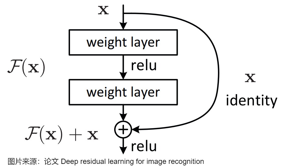
Annotated crop of Figure 2 from He et al.’s ResNet paper. The curved edge is an identity shortcut and the rectangular path is $F(x)$. The figure’s post-addition ReLU belongs to that ResNet-v1 block; it is not a universal rule for Transformer residual/normalization order.

0x06C Why The Backward Path Changes

Let $L$ be a scalar loss and use column-vector gradient convention. From $y=x+F(x)$,

$$\nabla_x L = \left(I+J_F(x)\right)^\top\nabla_y L,$$

where $J_F(x)=\partial F/\partial x$. Expanding the product gives

$$\nabla_x L = \nabla_y L + J_F(x)^\top\nabla_y L.$$

The first term is a direct identity contribution; the second traverses the learned branch. A plain block $y=F(x)$ has only the second term.

For a stack

$$x_{\ell+1}=x_\ell+F_\ell(x_\ell),$$

the end-to-end Jacobian contains

$$\frac{\partial x_L}{\partial x_0} = \prod_{\ell=0}^{L-1} \left(I+J_{F_\ell}(x_\ell)\right).$$

This product is not automatically well conditioned. Residual paths add an identity term to each local Jacobian, but large, adversarial, or poorly scaled branch Jacobians can still produce unstable products. Initialization, normalization, residual scaling, optimizer behavior, and block ordering still matter. Residual streams and normalization develops those choices in complete blocks.

0x06D Residual Does Not Mean “Preserve Everything”

The output is a sum, not a protected copy stored beside the branch. Later layers receive $x+F(x)$ and can modify it again. A residual route makes an identity contribution available to the optimization path; it does not guarantee that semantic features remain unchanged or that gradients never vanish.

Claim	Verdict	Reason
“Residuals solve the degradation problem in the source experiments.”	source-reported	residual nets reduced training error relative to comparable plain deep nets
“Residuals guarantee successful optimization.”	false generalization	the Jacobian product and the optimizer still matter
“Residuals create long-range token interaction.”	false	elementwise addition preserves row ownership; the branch must perform routing/mixing
“Projection and identity shortcuts are equivalent.”	false	projection changes parameters, compute, and possibly representation
“The original ResNet block fixes Transformer norm order.”	false	Transformer block assembly is a separate design contract

0x06E ConvS2S Already Combined The Threads

ConvS2S is a useful pre-Transformer junction. Its convolutional blocks used GLUs for channel gating and residual additions for depth, while every decoder layer performed source attention. The model therefore separated three jobs:

convolution  -> fixed local/depth communication
attention    -> target-conditioned source addressing
residual     -> additive depth path

The jobs cooperate but are not aliases. A residual connection does not choose which source token to read. Attention does not by itself provide a depth- identity route. A GLU gates channels in the convolutional update; it is not the same state machine as a GRU.

0x06F One Schema For The Competing Paths

Reconstructed interface diagram. It compares dependency-graph paths under explicit teaching assumptions: a recurrent chain, causal width-three contiguous convolution, width-two doubling dilation, and an elementwise residual stack. It does not compare measured latency or model quality. The ConvS2S strip records that its actual decoder combined convolution, GLU, residual addition, and per-layer attention.

The corresponding contract table is:

Mechanism	State exposed per position	Same-layer time dependency	Distant communication path	Main design alternative
vanilla/gated recurrence	one loop-carried state per step	$h_t$ requires $h_{t-1}$	$O(\Delta)$ recurrent transitions	GRU/LSTM, bidirectionality, source reversal
contiguous causal convolution	one row per layer/position	rows in one layer are parallel	$\lceil\Delta/(k-1)\rceil$ layers	kernel width and depth
doubling dilated convolution	one row per layer/position	rows in one layer are parallel	logarithmic depth under the stated schedule	dilation cycle and coverage pattern
residual update	same row set as branch input/output	inherited from $F$	adds an identity depth route; no new cross-row edge	identity, projection, scaling/gating
ConvS2S decoder	convolutional rows plus encoder memory	target rows batchable in teacher-forced training	local depth path plus per-layer source attention	number of layers, kernel width, attention placement

“Parallel” in this table refers to known rows within one layer. Autoregressive generation still discovers target tokens sequentially. Runtime kernels, hardware utilization, and cache strategies can change wall-clock behavior without changing these dependency edges.

0x06G Bringing The Paths Together

The historical contribution is now precise:

• recurrence supplies a learned loop-carried state, including gated variants;
• convolution supplies shared local operators and row-parallel layer evaluation, with depth/dilation controlling the field;
• residual learning supplies an additive identity route through deep stacks;
• attention supplies content-conditioned access to a set of states.

The next step is to make attention the principal operation that mixes sequence positions, while retaining residual paths through depth. This brings the earlier ideas together without eliminating the reasons to use recurrence or convolution: locality, streaming, and memory requirements still matter.

0x07 Transformer: putting the pressures together

The Transformer is the synthesis point of this first movement, not a slogan that attention made every earlier idea obsolete. Vaswani et al. (2017) removed sequence-aligned recurrence and convolution from the principal transduction path. Their actual model still required embeddings, position, residual routes, normalization, position-wise feed-forward transformations, an output head, and an autoregressive decoder contract.

This raises a practical question:

Which computation graph did the Transformer assemble from the earlier pressures, and what do its work, sequential-depth, and path-length claims establish before any hardware benchmark is run?

0x07A The Transformer Is A Synthesis, Not Attention Alone

The route reconstructed so far contributes four different contracts:

Earlier mechanism	What the Transformer keeps	What it changes
recurrent sequence models	a conditional sequence objective and causal output factorization	no loop-carried hidden state is required between rows inside one layer
convolutional sequence models	row-parallel training and shared transformations	content-conditioned routing replaces the fixed local kernel as the principal row-mixing operation
residual networks	additive identity routes through depth	the learned residual branch can now route between sequence rows
encoder-decoder attention	query-conditioned retrieval from a visible memory	self-attention turns that read into an internal sequence operation

The comparison below summarizes three communication patterns, but it suppresses masks, convolution schedules, residual branches, and hardware effects. It is a communication cartoon, not a runtime result.

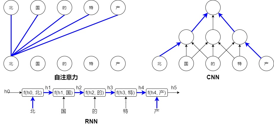
The original encoder-decoder object graph makes the missing pieces visible:

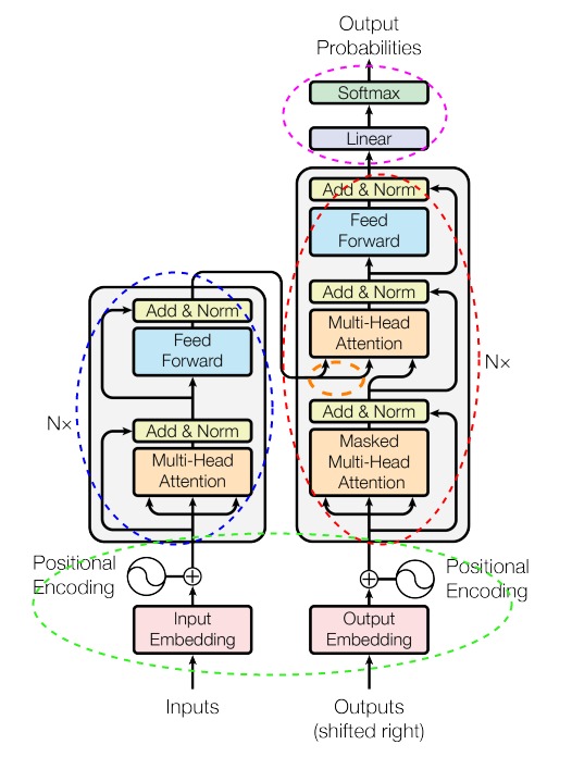
The figure annotates the original 2017 encoder-decoder with post-residual normalization. It is not a universal modern Transformer topology: decoder-only models remove the encoder/cross-attention path, and later models change normalization, position, feed-forward, and attention details.

0x07B One Layer Alternates Routing And Row-Wise Transformation

Let a batch of sequence states be

$$X^{(\ell)}\in\mathbb{R}^{B\times n\times d}.$$

At the bottom of the stack, token embeddings and a position representation have compatible shapes so that the row identities are not lost:

$$X^{(0)}=E[\text{tokens}]+P, \qquad E[\text{tokens}],P\in\mathbb{R}^{B\times n\times d}.$$

Ignoring dropout and normalization placement for one bounded derivation, an encoder layer alternates two residual updates:

$$\widetilde X^{(\ell)} =X^{(\ell)}+ \operatorname{Route}^{(\ell)}\!\left(X^{(\ell)},M\right),$$ $$X^{(\ell+1)} =\widetilde X^{(\ell)}+ \operatorname{Channel}^{(\ell)}\!\left(\widetilde X^{(\ell)}\right).$$

Route is self-attention: it can mix information between rows permitted by the visibility mask $M$. Channel is the position-wise feed-forward network: it applies the same learned transformation to each row and does not create a new cross-row edge. The original paper applied layer normalization after each residual addition; pre-norm, post-norm, and modern block recurrences are derived in M3.7.

The decoder inserts a third operation family:

encoder layer:
    source self-route -> row-wise channel transform

decoder layer:
    causal target self-route
    -> source cross-route
    -> row-wise channel transform

The tensor ownership is different at each route:

Route	Query rows	Memory rows	Visibility
encoder self-attention	source states $[B,n_s,d]$	same source states	all unmasked source rows
decoder self-attention	target states $[B,n_t,d]$	same target states	causal target prefix
encoder-decoder attention	target states $[B,n_t,d]$	encoder output $[B,n_s,d]$	valid source rows

This is the conceptual object graph, not the projected $Q/K/V$ derivation. 0x08 introduces those roles; M3 derives multi-head packing, normalization, position, and exact block order.

Attention mixes information between permitted rows; the feed-forward network transforms each row independently. Normalization and dropout are omitted to make these two operations and their residual paths visible.

A code-level skeleton keeps that separation executable:

def encoder_layer(x, source_mask, self_route, channel, norms):
    # x: [B, n_source, d]
    routed = self_route(query=x, memory=x, mask=source_mask)
    x = norms[0](x + routed)                # original 2017 post-norm order
    changed_per_row = channel(x)            # [B, n_source, d]
    return norms[1](x + changed_per_row)


def decoder_layer(y, encoder_memory, causal_mask, source_mask,
                  self_route, cross_route, channel, norms):
    # y: [B, n_target, d]; encoder_memory: [B, n_source, d]
    y = norms[0](y + self_route(y, y, causal_mask))
    y = norms[1](y + cross_route(y, encoder_memory, source_mask))
    return norms[2](y + channel(y))

Each entry in norms is a separate normalization module with its own learned affine parameters. The pseudocode follows the paper’s operation order, but is not a drop-in implementation: projection parameters, heads, dropout, padding conventions, and cache behavior remain intentionally absent.

0x07C Internal Non-Recurrence Does Not Remove Autoregressive Output

The encoder can update known source rows together. During teacher-forced training, all shifted target inputs are also known, so one causal decoder pass can score all next-token factors:

decoder input:  <bos>  y_1  y_2  ...  y_(m-1)
supervision:           y_1  y_2  ...  y_m
visibility at row t:   target rows <= t only

At generation time, $y_t$ is not known before it is selected. The output loop therefore remains:

$$y_t\sim p_\theta(\,\cdot\mid y_{<t},X_{source}), \qquad t=1,2,\ldots$$

The precise claim is:

The Transformer removes the recurrent hidden-state dependency from an internal sequence layer; it does not make autoregressive token discovery parallel.

This distinction explains why processing a supplied prompt and generating its continuation require different schedules. We return to those phases in 0x0B.

0x07D Four Quantities Hidden Inside “Efficient”

The original paper’s Table 1 compares three graph quantities. Hardware adds a fourth that the table does not predict:

Quantity	Question it answers	It does not answer
leading arithmetic work	how the selected operation count grows with $n,d,k,r$	exact FLOPs of a complete layer
minimum sequential depth	how many dependent stages prevent same-example parallel evaluation	accelerator occupancy or launch cost
maximum graph path	how many learned edges connect distant positions under a stated graph	whether the learned weight on that path is useful
wall-clock runtime	how long one implementation takes on one workload/hardware/software stack	a hardware-independent architectural theorem

Memory capacity and traffic are additional ledgers. A constant graph path can still use an expensive dense matrix; fewer arithmetic terms can still run slowly if the kernel is serial, launch-bound, bandwidth-bound, or poorly utilized. M4 will reconcile full FLOPs, bytes, kernels, and measured time.

Asymptotic arithmetic is not wall-clock runtime. It supplies a growth contract; runtime requires a concrete tensor shape, implementation, software stack, and device.

0x07E Deriving The Paper’s Leading Work Terms

Use $n$ sequence rows of width $d$. Count scalar multiply-accumulate terms only up to asymptotic order.

Recurrent layer. Each of $n$ time steps applies at least one dense $d\times d$ state transform. One transform contributes order $d^2$, so

$$n\times O(d^2)=O(nd^2).$$

The states form a chain, giving $O(n)$ sequential stages and a worst-case $O(n)$ path between distant positions. Gates add constant numbers of dense transforms; they do not change these orders.

Dense self-attention interaction. There are $n$ query rows and $n$ key rows. Each pair computes a width-$d$ compatibility term, so

$$(n\times n)\times O(d)=O(n^2d).$$

Mixing values over the same pair graph contributes another term of the same order. All known rows can participate in batched matrix operations, giving $O(1)$ sequential stages at the layer abstraction. Every allowed pair has a one-layer graph edge, giving $O(1)$ maximum path in dense bidirectional self-attention. A causal mask makes the graph directed: a later row can read an earlier row, but not conversely.

Dense convolution. At each of $n$ output rows, a width-$k$ kernel combines $k$ input rows through dense channel transforms. The leading term is

$$n\times k\times O(d^2)=O(knd^2).$$

Rows in one layer can be evaluated together, but a kernel narrower than the sequence needs depth before distant positions share a path.

Restricted self-attention. If each row may inspect only $r$ memory rows, the pair count falls from $n^2$ to $nr$:

$$(n\times r)\times O(d)=O(rnd).$$

Overlapping neighborhoods then require depth proportional to $n/r$ to relay information across the full sequence. This scaling assumes local-only edges; global read/write routes can change the graph diameter itself, not just a constant factor. Within the local-only case, constants depend on whether the window is causal, centered, dilated, or augmented with global rows.

The paper’s comparison is therefore:

Layer type	Leading work per layer	Sequential operations	Maximum path under stated graph
self-attention	$O(n^2d)$	$O(1)$	$O(1)$
recurrent	$O(nd^2)$	$O(n)$	$O(n)$
convolutional, dilated stack	$O(knd^2)$	$O(1)$	$O(\log_k n)$
restricted self-attention	$O(rnd)$	$O(1)$	$O(n/r)$

These rows reproduce the paper’s abstraction. They omit input/output projections, feed-forward work, normalization, residual additions, materialized intermediates, backward passes, optimizer state, and kernel-specific traffic.

0x07F The n < d Crossover Is A Selected-Term Comparison

Comparing only the interaction term $n^2d$ with the recurrent state term $nd^2$ gives

$$n^2d<nd^2.$$

For positive $n$ and $d$, divide both sides by $nd$:

$$n<d.$$

This is the origin of the paper’s statement that self-attention’s selected leading term is smaller when sequence length is below representation width. It is not a proof that a complete self-attention layer is faster.

n=128, d=512
pair count n^2:                 16,384
self-attention term n^2*d:  8,388,608
recurrent term n*d^2:      33,554,432

n=2048, d=512
pair count n^2:              4,194,304
self-attention term n^2*d: 2,147,483,648
recurrent term n*d^2:        536,870,912

The examples reverse because $128<512$ while $2048>512$. They still exclude the projections and position-wise feed-forward network in a Transformer layer, the constant factors inside a recurrent cell, parallel occupancy, memory traffic, and implementation quality. The correct label is selected-term crossover, not “attention is always faster.”

0x07G Path Length Depends On The Graph Assumption

A contiguous causal convolution of width $k$ expands its receptive field by $k-1$ earlier positions per layer. After $L$ layers,

$$R_L=1+L(k-1).$$

To span $n$ positions,

$$L\geq\left\lceil\frac{n-1}{k-1}\right\rceil,$$

which the Transformer paper summarizes as $O(n/k)$. For $n=9$ and $k=3$, four contiguous layers are required: $1+4(3-1)=9$.

A different result requires a different schedule. Let a width-$k$ causal stack use dilations $1,k,k^2,\ldots,k^{L-1}$. Its receptive field is

$$R_L =1+(k-1)\sum_{j=0}^{L-1}k^j =1+(k^L-1) =k^L.$$

Therefore $L\geq\lceil\log_k n\rceil$. With $k=2$ and $n=8$, three layers span eight rows. The paper’s $O(\log_k n)$ convolutional table entry assumes this kind of dilated route; a contiguous stack does not inherit it.

Dense self-attention instead places an allowed pair edge in one layer. That is a shorter graph route, not a guarantee of perfect memory, nonzero learned weight, numerical stability, or causal access to the future.

0x07H Dense And Restricted Attention Change The Pair Graph

The pair graph makes the trade visible. Dense bidirectional attention permits $n^2$ query-memory pairs. Causal attention permits $n(n+1)/2$ pairs including the diagonal. A fixed restricted neighborhood permits order $nr$ pairs.

Reconstructed comparison. Every formula is tied to a graph assumption. The rightmost runtime boundary is intentionally not inferred from asymptotic work.

Reducing allowed pairs can reduce arithmetic and temporary score state, but removed edges must be replaced by depth, dilation, global tokens, recurrence, compression, or another route if distant information must still communicate. That design space leads to sparse attention, state-space layers, and hybrids; it is not evidence that one graph dominates every workload.

0x07I What The Transformer Did Not Solve

Moving routing into dense attention exchanges old constraints for new ones:

• quadratic pair work: exact dense attention evaluates every legal pair;
• autoregressive output dependency: causal generation still discovers one unknown token after another;
• position: row mixing alone does not encode order, so positional geometry must enter the model;
• persistent serving state: efficient decoding retains prior K/V state, which creates capacity and bandwidth pressure;
• locality and streaming: dense global routing may be a poor inductive or systems fit for high-rate local signals and bounded-memory streaming;
• deep optimization: residual paths help, but normalization, initialization, precision, data, and optimizer behavior still govern trainability.

IO-aware kernels can avoid writing a full score matrix to slow memory, sparse graphs can remove pairs, and caching can avoid recomputing old K/V rows. None of those changes makes the original constraints disappear; each changes a specific work, traffic, state, or path contract owned by later modules.

0x07J Why Alternative Information Paths Remain

The architecture choice is a menu of different state and visibility contracts:

Mechanism	Strong property	Design cost or limitation
gated recurrence	compact carried state and natural streaming	loop-carried training dependency; content is compressed into state
contiguous/dilated convolution	local prior, row-parallel layers, regular access	field and distant path are fixed by kernel/depth schedule
dense attention	direct content-conditioned routing among legal rows	pairwise work/state grows with sequence length
sparse/local attention	fewer pair edges and controlled visibility	distant access needs depth or explicit global routes
structured state-space layer	long state evolution with parallel training algorithms	retrieval and state semantics differ from explicit pair routing
hybrid block	local, stateful, and global routes can coexist	more ownership, kernel, and tuning complexity

S4 and Mamba revisit state evolution with structured or selective updates and parallel training algorithms. They are not the fixed-context encoder-decoder prototype under a new name. Convolution-attention hybrids likewise recognize that local filtering and global retrieval solve different subproblems.

The durable conclusion is not “attention replaced everything”:

Choose the information path whose visible state, graph distance, arithmetic, and runtime contract fit the workload, then state the assumptions that make the comparison true.

0x07K From The Architecture To An Attention Read

The graph explains how information moves; the leading work terms explain how selected operations grow. They are useful for different decisions. Changing the graph can change what information is available, whereas changing a kernel can leave the mathematical operation intact while altering how it executes.

The attention chapters develop the projected computation; the cost model connects it to complete parameter, memory, and operation accounting. First, we need to look inside one read. Query, key, and value separate the request, the matching representation, and the information returned.

0x08 Q, K, And V: Request, Address, And Payload

The historical sequence-to-sequence context vector gives us the right intuition, but the Transformer needs an interface that can be reused at every layer and every query row. To understand the read before choosing its implementation, ask:

Before choosing a score function, projection width, mask representation, or number of heads, what computational role does each of query, key, and value play, and which row owns the returned state?

The three roles are request, address, and payload. These are roles in one read operation, not three ontological kinds of token and not yet the complete scaled-dot-product implementation.

0x08A From Exact Lookup To Differentiable Addressing

An ordinary lookup table stores pairs:

key -> value

A hard lookup receives one query, finds an exactly matching key, and returns the paired value. A soft addressable read changes three assumptions:

1. matching can be learned rather than exact;
2. several keys can match with different strengths;
3. the result can contract several payloads into one output.

For query row i and memory row j, let a generic matcher produce

$$s_{ij}=\operatorname{match}(q_i,k_j).$$

Let $\mathcal{V}(i)$ be the memory rows visible to query i. Normalization is over that row’s visible keys:

$$\alpha_{ij} = \frac{\exp(s_{ij})} {\sum_{\ell\in\mathcal{V}(i)}\exp(s_{i\ell})}, \qquad j\in\mathcal{V}(i),$$

and $\alpha_{ij}=0$ for a hidden row. The output owned by query i is

$$o_i=\sum_{j\in\mathcal{V}(i)}\alpha_{ij}v_j.$$

With dot-product matching and the Transformer’s scale factor, the same read is commonly written in matrix form as

$$\operatorname{Attention}(Q,K,V) = \operatorname{softmax}\!\left(\frac{QK^\mathsf{T}}{\sqrt{d_k}}\right)V$$

Here the rows of $Q$ ask questions, the rows of $K$ provide addresses, and the rows of $V$ supply the content to combine; $d_k$ is the query/key width. The displayed formula assumes all represented key rows are visible. A causal or padding restriction must be applied to the scores before normalization. Every active query also needs at least one visible key; otherwise the softmax read is undefined and requires an explicit implementation policy. Scaled dot-product attention derives the projections, scale, and masked score path. We first make the roles of these arrays explicit.

0x08B Which Rows Ask, Match, And Contribute

Role	Question answered	Rows and axes	It is not
query	What is this row asking for?	query row i owns output row o_i	the returned content
key	How should memory row j advertise itself?	keys occupy the normalization / address axis	a database key that must match exactly
value	What should memory row j contribute if selected?	value row j is paired with key row j	evidence used only for matching

The separation matters because matching and contribution are different jobs. A memory row may advertise tense or syntactic role through its key while contributing a different semantic payload through its value. A target row may need another representation to express what information it currently lacks. Learned transformations can construct these roles from hidden state without claiming that the hidden row itself permanently “is” a query, key, or value.

Four invariants apply to this read:

score table ownership:
    rows are queries; columns are candidate memory keys

normalization axis:
    visible key columns for one fixed query row

payload pairing:
    key row j and value row j refer to the same memory row

returned row ownership:
    one output row per query row, even when memory has another length

0x08C A Numeric Vector Read, Not Merely A Score Example

Take one query, three visible memory rows, and matcher scores [1.2, 0.2, -0.4]. Their row softmax is approximately [0.637, 0.234, 0.129]. Now make the payloads explicit:

v_1 = [ 2, 0]
v_2 = [ 0, 4]
v_3 = [-1, 2]

Then

$$\begin{aligned} o &=0.637[2,0]+0.234[0,4]+0.129[-1,2]\\ &\approx[1.15,1.19]. \end{aligned}$$

The output is not the highest-scoring key, the score vector, or a selected token ID. It is a weighted contraction of value rows. Changing v_3 changes the returned content without changing the three match scores; changing k_3 can change its weight without directly specifying its payload. That counterfactual is the practical reason to keep address and payload separate.

A code-level skeleton keeps the axis visible:

def bounded_read(query_rows, memory_rows, visible, match, key_of, value_of):
    outputs = []
    for i, query_row in enumerate(query_rows):
        candidate_rows = [
            j for j in range(len(memory_rows)) if visible[i][j]
        ]
        scores = [
            match(query_row, key_of(memory_rows[j]))
            for j in candidate_rows
        ]
        if not candidate_rows:
            raise ValueError("An active query needs at least one visible key")
        weights = softmax(scores)  # normalization is over candidate_rows
        output_i = sum(
            weight * value_of(memory_rows[j])
            for weight, j in zip(weights, candidate_rows)
        )
        outputs.append(output_i)   # output_i remains query-row owned
    return outputs

The matcher and key/value transformations can change without changing the output’s relationship to its query row. The later attention chapters develop these choices.

0x08D Self-Read And Cross-Read Reuse The Roles

In self-attention, query and memory roles are constructed from the same row set. In cross-attention, the query stream and memory stream differ:

Route	Query rows	Key/value rows	Score-table shape	Returned rows
encoder self-read	source state [B,S,d]	the same source state	source by source	[B,S,*]
decoder self-read	target state [B,T,d]	the same target state	target by target	[B,T,*]
encoder-decoder cross-read	target state [B,T,d]	encoder memory [B,S,d]	target by source	[B,T,*]

The star marks a payload/output width deliberately left to M3. A cross-read does not become source-owned merely because it reads source memory: its T queries still produce T returned rows.

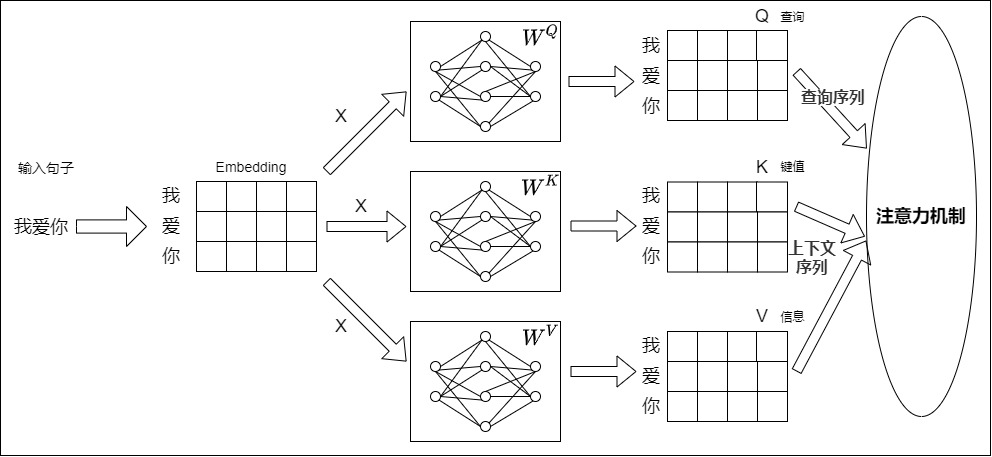
The figure shows one same-stream projection path and uses Chinese labels for query, key, value, and attention. It establishes that the roles can be learned from one hidden row set; it does not establish the exact scale, head layout, mask convention, parameter share, or modern runtime schedule.

0x08E Different Implementations Of The Same Read

The role contract leaves real alternatives open:

Design coordinate	Some valid choices	What changes
query/memory source	same stream; separate streams	self-read versus cross-read ownership
matcher	additive; dot; bilinear; kernelized or other learned score	score arithmetic and geometry
addressability	dense; local; sparse; hard/top-k	visible candidates and execution schedule
key/value relation	separate transforms; tied or shared variants	what matching can ignore or expose
payload aggregation	convex weighted sum; gated or structured variants	returned-state semantics

These choices explain why Q/K/V describe an interface rather than one final formula. M3.1 derives projected tensors, scaling, masks, stable softmax, and the exact value contraction. M3.2 derives head packing, output fusion, and cross-attention modules. M4 and M5 then analyze their computational cost and runtime execution.

0x09 Choosing a Transformer family is choosing an execution contract

“Transformer” does not identify one input/output program. The useful question is therefore not “which family is best?” but:

Which query rows may read which state rows, which outputs are supervised or generated, and which state must persist when the same weights move from training to runtime?

Encoder-only, decoder-only, encoder-decoder, and prefix/unified stacks reuse related operations while answering that question differently.

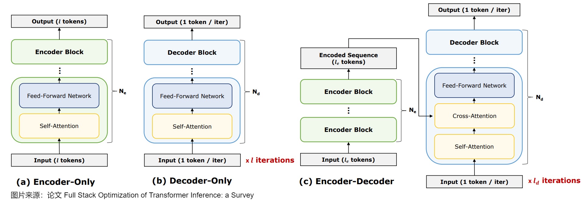
The figure compares three arrangements of encoder, decoder, and cross-attention modules, but its decoder labels say 1 token / iter. Read that only as an incremental generation view. Decoder-only training and prompt prefill normally process many known rows in one forward; the architecture name does not require one-token input for every phase.

0x09A Visibility Is A Row-By-Column Contract

Let $R$ be the query-row set and $C$ the candidate key-row set. A structural visibility matrix

$$G\in\{0,1\}^{|R|\times|C|}$$

uses query rows on its vertical axis and key rows on its horizontal axis. $G_{ij}=1$ means query row i may read memory row j; it does not mean that the learned attention weight must be large.

Padding is another predicate. If $K_j$ records whether key row j contains valid state, the key-side read mask is

$$A_{ij}=G_{ij}\land K_j.$$

In plain notation:

effective[i][j] = structural[i][j] and key_valid[j]

Query validity is a separate concern. A padded query row can be prevented from contributing to a loss or downstream output even though an implementation temporarily computes it. Masking only invalid query rows does not stop valid queries from reading padded keys.

The core oracle is therefore small:

def compose_read_mask(structural, key_valid):
    # structural: [n_query, n_key]
    # key_valid: [n_key]
    return [
        [structural[i][j] and key_valid[j] for j in range(len(key_valid))]
        for i in range(len(structural))
    ]

Mask polarity and representation remain implementation choices. Some kernels consume booleans, some consume additive 0 / -inf bias, and some encode causality in the kernel schedule. The relation above is the semantic contract.

0x09B Full And Causal Self-Visibility

For a non-padding sequence of length $n$, full self-visibility is

$$G^{\text{full}}_{ij}=1,$$

while left-to-right causal visibility is

$$G^{\text{causal}}_{ij}=\mathbf{1}[j\le i].$$

With five rows, the two relations are:

FULL SELF-VISIBILITY          CAUSAL SELF-VISIBILITY
q\k  0 1 2 3 4               q\k  0 1 2 3 4
 0   1 1 1 1 1                0   1 . . . .
 1   1 1 1 1 1                1   1 1 . . .
 2   1 1 1 1 1                2   1 1 1 . .
 3   1 1 1 1 1                3   1 1 1 1 .
 4   1 1 1 1 1                4   1 1 1 1 1

The diagonal is legal because a training input row contains the token available at that position and normally predicts a shifted label. For input [<bos>, x_1, x_2], the corresponding labels can be [x_1, x_2, x_3]. Processing all three rows together does not expose x_3 to the row that must predict it.

0x09C Encoder-Decoder Uses Three Relations, Not One Matrix

Let the source have length S=3 and shifted target input have length T=4. The original encoder-decoder Transformer composes three different reads:

SOURCE SELF [S,S]      TARGET SELF [T,T]       TARGET -> SOURCE [T,S]
q\k s0 s1 s2           q\k y0 y1 y2 y3        q\k s0 s1 s2
s0   1  1  1           y0   1  .  .  .         y0   1  1  1
s1   1  1  1           y1   1  1  .  .         y1   1  1  1
s2   1  1  1           y2   1  1  1  .         y2   1  1  1
                       y3   1  1  1  1         y3   1  1  1

Source self-read constructs source memory. Target self-read preserves the left-to-right target boundary. Cross-read lets every target query read all valid source memory rows. Source padding can still remove columns from the cross matrix; target causality does not apply along the source axis.

This tensor ownership explains the runtime state:

source IDs [B,S]
    -> encoder once
        -> source memory [B,S,d]
            -> retained while target rows are generated

shifted target IDs [B,T]
    -> causal target self-read
    -> cross-read over retained source memory
        -> target-owned states [B,T,d]

0x09D Prefix LM Is A Fourth Visibility Contract

A prefix language model uses one row stream but gives a supplied prefix and a generated target different visibility. Let the first $P$ rows be prefix rows. Then

$$G^{\text{prefix}}_{ij}=1$$

exactly when either:

1. i < P and j < P: prefix queries read the full prefix; or
2. i >= P and (j < P or j <= i): target queries read all prefix rows and the causal target prefix.

For P=3 and two shifted target-input rows:

q\k  p0 p1 p2 y0 y1
 p0   1  1  1  .  .
 p1   1  1  1  .  .
 p2   1  1  1  .  .
 y0   1  1  1  1  .
 y1   1  1  1  1  1

This is not the same object graph as encoder-decoder. There is one stack and one block visibility relation rather than a separate source stack, target stack, and cross-attention module. The conditioning set can be similar while parameter ownership, intermediate state, and runtime scheduling differ.

UniLM demonstrated that bidirectional, unidirectional, and sequence-to-sequence objectives can be controlled in a shared Transformer with attention masks. T5 separately compared a decoder-only prefix LM with encoder-decoder variants, then used an encoder-decoder architecture for its main text-to-text system. Those papers support a mask-program design space; they do not prove that every mask program trains or serves equivalently. (Dong et al., 2019, Raffel et al., 2020)

Reconstructed visibility contract. A colored cell means a read is permitted, not that its learned weight is nonzero or important. Padding and packed-sample boundaries compose with these structural matrices.

0x09E Family Names Are Shorthand For Four Independent Contracts

Contract	Question	A family name alone does not determine
architecture	Which parameter-owning stacks and cross-stream modules exist?	training objective or decoding policy
visibility	Which query rows may read which key rows?	whether a permitted edge receives high weight
objective/output	Which rows are supervised and what object should they produce?	runtime batching or cache layout
runtime	Which inputs are known together and which decisions must be fed back?	model quality or task suitability

Encoder-only: full-context representation

An encoder-only stack normally lets each valid input row read valid rows on both sides:

input IDs [B,S]
    -> full-visibility encoder blocks
        -> contextual states [B,S,d]

Its natural product is a representation: per-row states, a pooled state, or a task head’s result. BERT is a primary example of deep bidirectional representations trained with masked-token and next-sentence objectives, but “encoder-only” is not synonymous with masked language modeling. Contrastive, classification, token-labeling, and other losses can consume the same architecture. (Devlin et al., 2018)

Decoder-only: causal continuation

A decoder-only stack normally places prompt and continuation in one causal stream:

known prefix IDs [B,T]
    -> causal decoder blocks
        -> hidden states [B,T,d]
            -> next-token logits [B,T,V]

During teacher-forced training, T can be the complete shifted training sequence and every row can execute together under the triangular relation. During generation, unknown outputs must be selected and appended one at a time, although the supplied prompt is normally processed as a multi-row prefill. GPT’s generative pre-training is a primary causal example; it does not make “decoder-only” a synonym for one-token matrix execution. (Radford et al., 2018)

Encoder-decoder: source memory plus target generation

An encoder-decoder keeps source and target state separate:

source -> full encoder -> retained source memory
target prefix -> causal decoder -> cross-read source -> target logits

The original Transformer used this contract for translation. T5 retained it for a unified text-to-text interface: task input is encoded, then target text is generated causally while reading encoder memory. The architecture is a natural fit when input and output have distinct row ownership, modalities, lengths, or update lifecycles. It is not automatically more accurate or slower than a decoder-only model; those are empirical system claims requiring a matched comparison. (Vaswani et al., 2017, Raffel et al., 2020)

Prefix and unified masks: one stack, asymmetric row rights

A prefix LM makes supplied input rows mutually visible while keeping generated target rows causal. Unified-mask systems can select full, causal, or source-target block relations for different examples or objectives. This can reuse one parameter stack, but it does not erase the distinctions among input corruption, label placement, cache topology, or generation order.

0x09F Objectives Expose Conditioning, Not The Whole Architecture

For decoder-only next-token training:

$$\mathcal{L}_{AR} = -\sum_{t=1}^{T}\log p_\theta(x_t\mid x_{<t}).$$

For encoder-decoder training with source s and target y:

$$\mathcal{L}_{seq2seq} = -\sum_{t=1}^{T_y}\log p_\theta(y_t\mid y_{<t},s).$$

A prefix LM can expose the same probabilistic conditioning while implementing it in one stack:

$$\mathcal{L}_{prefix} = -\sum_{t=1}^{T_y}\log p_\theta(y_t\mid y_{<t},p),$$

where p occupies the fully visible prefix block. Similar conditioning does not imply identical parameters or execution.

For masked-token encoder training, let $M$ be selected prediction positions and $\tilde{x}$ the corrupted input:

$$\mathcal{L}_{MLM} = -\sum_{i\in M}\log p_\theta(x_i\mid\tilde{x}).$$

Full visibility does not leak the answer when the original token at a selected position has been hidden or replaced by the corruption procedure. Conversely, a causal architecture does not become a valid next-token trainer unless labels are shifted and loss rows are aligned correctly. Visibility, corruption, labels, and reduction are separate contracts.

0x09G Training, Prefill, And Decode Execute Different Extents

Family	Training extent	Initial inference work	Repeated generation work	Persistent state
encoder-only	supplied rows together	supplied rows together	none unless an external loop is added	task-dependent representations
decoder-only	shifted rows together under causal visibility	prompt prefill over many rows	one or more newly proposed rows under the decoding algorithm	prefix-dependent runtime state
encoder-decoder	source rows and shifted target rows together in their stacks	encode source, then initialize target	target generation while reading retained source	source memory plus target-prefix state
prefix LM	prefix and shifted target rows under a block mask	full prefix prefill	causal target generation	prefix/target state in one stack

The matrix width of a decoder forward therefore depends on phase. “Causal” describes legal dependencies; it does not require every training or prefill forward to have one input row. M3.9 develops shifted labels, loss, backward, and parameter updates. M3.10 develops prefill, decode, selection, cache state, and termination.

0x09H Paper Variants Compared By Contract

Paper/system	Parameter topology	Structural visibility	Training signal highlighted here	Natural returned object
original Transformer	encoder stack + decoder stack + cross-read	full source; causal target; target reads source	source-conditioned next-target prediction	target logits
BERT	encoder stack	full valid input context	corrupted/masked-token representation learning	contextual representations / task head
GPT generative pre-training	decoder stack	causal single stream	next-token likelihood	continuation logits
UniLM	shared Transformer stack	mask-selected bidirectional, causal, or seq2seq relation	multiple language-model objectives	objective-dependent
T5 baseline	encoder-decoder	full source; causal target; target reads source	text-to-text denoising and supervised tasks	target text logits
T5 prefix-LM comparison	decoder stack	full prefix block + causal target block	prefix-conditioned language modeling	continuation logits

This is a contract comparison, not a benchmark ranking. Dataset, corruption, parameter count, optimization, and hardware differ across the papers.

0x09I When Valid Shapes Hide Incorrect Visibility

Failure	Shape may still work because	Semantic result
transpose the visibility matrix	square self-attention remains [n,n]	query/key ownership reverses for asymmetric masks
mask padded query rows but not padded key columns	both masks broadcast	valid queries can still read padding
remove the causal triangle during teacher forcing	all target rows are present	a row reads future target inputs and leaks labels
apply target causality to cross-attention source columns	target and source masks can broadcast	legal source evidence is incorrectly hidden
call every full-visibility stack “BERT”	architecture shape resembles an encoder	objective, corruption, and output contract disappear
call every causal call “one-token decode”	causality is present in all phases	training and prefill parallelism are misdescribed
treat prefix LM as encoder-decoder	conditioning set can look similar	parameter owners and runtime state topology are wrong

0x09J From Family Choice To Implementation

A family name is useful shorthand once the modules, permitted reads, outputs, and execution phases are explicit. It is not a substitute for any of them.

Name the row owners, write the visibility matrix, identify the supervised or generated rows, and state which inputs are known together at runtime. Only then use a family label.

We can now follow these decisions into actual module objects and the tensors that pass between them. This is where a diagram becomes a program, and where matching dimensions can conceal a different architecture.

0x0A From text to a running model: objects first, tensors second

An architecture diagram names conceptual components. A program must construct concrete objects, register parameters or buffers under those objects, and pass runtime tensors through typed interfaces. Those are three related graphs, not one picture:

build graph:       object -> child module -> persistent parameter / buffer
runtime graph:     input tensor -> activation -> output tensor
training graph:    parameter + saved activation -> gradient -> optimizer state

Start with construction, then follow one forward pass:

Which object owns each parameter, which stream owns each runtime row, and exactly where does an integer token ID become hidden state, vocabulary scores, a normalized distribution, and finally another integer ID?

The distinction matters because a model can be shape-correct and still be a different architecture. A reused Python object can tie weights accidentally; a source mask and target mask can share an extent while expressing opposite read rights; a hidden row and a logit row can both be floating-point arrays while permitting entirely different operations.

0x0A.1 The Build Graph Has Two Copy Boundaries

The simplified construction below follows the object layout of the Annotated Transformer. Its factory creates reusable templates, deep-copies them into semantic roles, then the Encoder and Decoder constructors deep-copy each layer template into a stack. This is pseudocode for object identity, not a runnable copy of the notebook: constructor options, imports, and initialization are omitted. The helpers and attribute names in the checks below are illustrative too.

def clones(module, N):
    return nn.ModuleList([copy.deepcopy(module) for _ in range(N)])


def make_model(src_vocab, tgt_vocab, N=6, d_model=512, d_ff=2048, h=8):
    c = copy.deepcopy
    attn = MultiHeadedAttention(h, d_model)
    ffn = PositionwiseFeedForward(d_model, d_ff)
    position = PositionalEncoding(d_model)

    encoder_layer = EncoderLayer(
        d_model,
        c(attn),                 # encoder self-attention role
        c(ffn),
    )
    decoder_layer = DecoderLayer(
        d_model,
        c(attn),                 # target self-attention role
        c(attn),                 # source-memory attention role
        c(ffn),
    )

    return EncoderDecoder(
        Encoder(encoder_layer, N),      # Encoder calls clones(layer, N)
        Decoder(decoder_layer, N),      # Decoder calls clones(layer, N)
        nn.Sequential(Embeddings(d_model, src_vocab), c(position)),
        nn.Sequential(Embeddings(d_model, tgt_vocab), c(position)),
        Generator(d_model, tgt_vocab),
    )

Removing c(attn) is not a cosmetic shortening. If the same attn object is passed as decoder self-attention and source-attention, both attributes can refer to the same parameter objects. Likewise, appending one layer object N times creates N calls to one tied layer, not an N-layer independently parameterized stack.

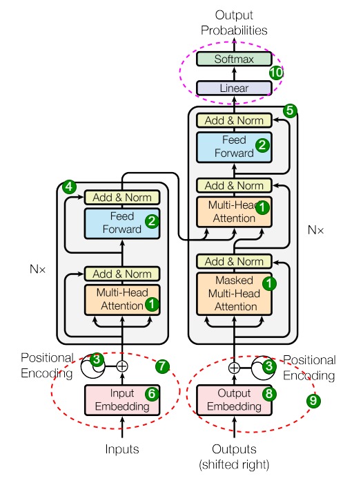
The numbered diagram maps conceptual blocks to factory arguments. It does not expose Python object identity. Its Add-and-Norm drawing follows the original paper’s post-norm architecture; the cited Annotated Transformer code instead places normalization before each sublayer. Matching module names does not make those two operation orders identical.

The object tree that the factory intends is:

EncoderDecoder
  src_embed
  encoder.layers[0..N-1]
    self_attn
    feed_forward
    residual / normalization wrappers
  tgt_embed
  decoder.layers[0..N-1]
    self_attn
    src_attn
    feed_forward
    residual / normalization wrappers
  generator

Every path names an owner. decoder.layers[2].self_attn and decoder.layers[2].src_attn perform related kinds of computation, but their query/memory contracts differ and the baseline construction gives them different parameters.

Templates are copied into separate roles and stack layers. The diagram distinguishes a reusable template, a role-specific copy, and a stack-layer copy. It is not a parameter count or internal attention calculation.

0x0A.2 Equal Values Are Not Shared Identity

deepcopy creates a different object containing copied values. Immediately after copying, two parameter tensors may be numerically equal while remaining different owners. Independent initialization or training can then make their values diverge. Numeric equality therefore cannot prove tying, and numeric difference is not required to prove independence.

An identity test inspects references and mutation isolation:

assert model.decoder.layers[0].self_attn is not \
       model.decoder.layers[0].src_attn
assert model.encoder.layers[0] is not model.encoder.layers[1]

p0 = model.encoder.layers[0].self_attn.q_weight
p1 = model.encoder.layers[1].self_attn.q_weight
assert p0 is not p1

# Immediately after cloning, equal values are permitted.
assert tensor_values_can_be_equal(p0, p1)
assert mutating_a_copy_does_not_change_the_other(p0, p1)

There are valid alternatives, but they must be selected deliberately:

Construction choice	Identity contract	Consequence
independent depth layers	layer[i].p is not layer[j].p	parameter count grows with depth; each layer can specialize
intentional depth sharing	several calls reference one parameter set	fewer unique parameters; repeated application is not the baseline independent stack
separate source and target embeddings	E_src is not E_tgt	vocabularies and representation tables may differ
target embedding/output tying	target lookup and vocabulary projection share a declared weight	input lookup and output scoring become one explicit parameter owner
accidental aliasing	references are shared without an architecture contract	silent model change, coupled gradients, and incompatible ownership assumptions

The important distinction is not “sharing is bad.” It is declared tying versus accidental aliasing. A tied architecture needs an explicit compatible shape, checkpoint contract, optimizer expectation, and paper/model claim. Parameter sharing is valid only when explicitly selected and documented at those boundaries.

0x0A.3 Parameters, Buffers, Activations, And Decisions Have Different Lifetimes

A module object is not the activation it produces. The same parameter can be called for many batches; each call produces new runtime tensors. A position module may also own a persistent non-trainable buffer. Masks and token IDs are runtime inputs rather than learned parameters.

Object	Example shape	Owner and lifetime	It is not
source embedding parameter	[V_src,d]	src_embed; checkpoint-persistent	source state for one batch
source state activation	[B,S,d]	current batch; source rows	the embedding table
encoder memory activation	[B,S,d]	current forward or retained runtime state; source rows	decoder output merely because decoder reads it
decoder hidden activation	[B,T,d]	current target rows	vocabulary scores
generator parameter	[V_tgt,d] plus bias	generator; checkpoint-persistent	logits for one batch
logits	[B,T,V_tgt]	current target rows and vocabulary channels	probabilities or selected IDs
probabilities	[B,T,V_tgt]	normalized runtime values	hidden state, despite sharing floating dtype
selected IDs	[B] for one next decision per request	generation policy / caller	an activation row with width d or V_tgt

M4 later prices persistent parameters, temporary activations, and training state separately. M5 later decides which runtime state persists across serving iterations. Here the purpose is to make the owners visible before cost and scheduling are introduced.

0x0A.4 Following A Small Batch Through The Model

Choose dimensions small enough to inspect:

B = 2       S = 7       T = 5       d = 16
V_src = 31  V_tgt = 37  N = 2       d_ff = 64

This deterministic example tracks shapes, row identities, and the distinction between IDs, hidden states, and vocabulary scores. Its transforms are synthetic: the selected IDs illustrate the final stage, not a trained model’s predictions.

Source lookup starts from integer IDs:

$$I^{src}\in\mathbb{N}^{B\times S}, \qquad X^{src}_{b,s,:}=E^{src}[I^{src}_{b,s}]+P_s \in\mathbb{R}^{d}.$$

Stacking the selected rows introduces hidden width but preserves the source axes:

$$X^{src}\in\mathbb{R}^{B\times S\times d}, \qquad M=\operatorname{Encoder}(X^{src},G^{src}) \in\mathbb{R}^{B\times S\times d}.$$

The target path starts from a different ID tensor and, in the untied baseline, a different lookup table:

$$I^{tgt}\in\mathbb{N}^{B\times T}, \qquad X^{tgt}\in\mathbb{R}^{B\times T\times d}.$$

The batch passes through these stages:

Stage	Shape	Dtype	Row owner	Semantic type
src_ids	[2,7]	integer	source	discrete vocabulary IDs
source_state	[2,7,16]	floating	source	initial hidden state
memory	[2,7,16]	floating	source	contextual source state
tgt_ids	[2,5]	integer	target	discrete vocabulary IDs
target_state	[2,5,16]	floating	target	initial hidden state
decoder_hidden	[2,5,16]	floating	target	contextual target state
logits	[2,5,37]	floating	target	unnormalized vocabulary scores
probabilities	[2,5,37]	floating	target	normalized vocabulary distribution
selected_next_ids	[2]	integer	target decision	discrete IDs; example result [28,21]

The source and target extents do not merge. The encoder produces S source rows. The decoder has T target queries, so reading S source memory rows still returns T target-owned rows:

cross-read score ownership:   target queries by source keys   [B,T,S]
cross-read returned rows:     one result per target query      [B,T,*]
decoder residual stream:      target-owned                     [B,T,d]

This is the same ownership invariant established abstractly in 0x08, now attached to the running object graph.

0x0A.5 The Generator Replaces Hidden Width With Vocabulary Width

Let decoder hidden state be

$$H\in\mathbb{R}^{B\times T\times d}$$

and let the generator own

$$W_{vocab}\in\mathbb{R}^{V_{tgt}\times d}, \qquad b\in\mathbb{R}^{V_{tgt}}.$$

For each batch and target row, the affine projection is

$$Z_{b,t,v} = \sum_{k=1}^{d}H_{b,t,k}W_{vocab,v,k}+b_v.$$

The contraction removes hidden channel k and introduces vocabulary channel v, hence

$$Z\in\mathbb{R}^{B\times T\times V_{tgt}}.$$

Softmax over v keeps that shape while changing the values from arbitrary scores to row-normalized probabilities. Selection over one chosen target row then returns integer IDs. Therefore:

decoder_hidden [B,T,d]
    is not logits [B,T,V_tgt]
    is not probabilities [B,T,V_tgt]
    is not selected_next_ids [B]

The return type must be checked in the implementation. In the cited Annotated Transformer, Generator.forward returns log-probabilities after log_softmax; its internal affine projection produces the logits. The example here displays those stages separately. Output heads and decoding compares their use in losses, weight tying, and token selection.

Solid boxes are batch-dependent tensors; dashed boxes are persistent parameter objects. The selected IDs come from the small deterministic example, not from a trained model.

0x0A.6 Checking More Than Shape

A small helper can record a tensor’s meaning alongside its shape and dtype:

@dataclass(frozen=True)
class TensorContract:
    name: str
    shape: tuple[int, ...]
    dtype: str
    row_owner: str       # source, target, or target_decision
    semantic_type: str   # IDs, hidden state, logits, probabilities

That extra metadata catches failures ordinary shape assertions miss:

def require_owner(tensor, expected, relation):
    if tensor.row_owner != expected:
        raise ValueError(
            f"{relation}: expected {expected}, got {tensor.row_owner}"
        )

require_owner(src_mask, "source", "cross_attention_key_mask")
require_owner(tgt_mask, "target", "decoder_self_attention_key_mask")

When S=T=5, both key-mask tensors can have shape [2,1,5]. Their stream tags still distinguish them, preventing target padding from controlling a source-memory read. Run the accompanying example with:

python3 docs/numinens-evidence/m1-1-architecture-orientation/architecture_oracle.py \
  --expected docs/numinens-evidence/m1-1-architecture-orientation/expected/tiny_execution_trace.json

0x0A.7 When Matching Shapes Hide A Different Program

Failure	Why a shallow check can pass	Semantic consequence
one attention object passed to decoder self- and cross-attention	both calls accept width d	gradients and updates tie two different routing roles
one layer object appended N times	every call returns [B,L,d]	apparent depth repeatedly applies one parameter owner
target key mask passed to cross-attention when S=T	both masks can be [B,1,L]	source-memory visibility is governed by target semantics
source memory and target hidden rows swapped when S=T	both can be [B,L,d]	returned row ownership and residual route are reversed
decoder hidden row sampled directly	floating tensor exists	axis d is treated as if it were vocabulary axis V_tgt
logits called probabilities	shape is unchanged by softmax	downstream code assumes normalization that has not occurred
selected ID called an activation row	both may be represented numerically	a discrete external decision is confused with differentiable model state

These failures justify carrying names, axes, owners, semantic types, and object identity together. Shape checks remain necessary, but they are not a complete execution contract.

0x0A.8 From A Forward Pass To Training And Generation

The trace connects token IDs to output decisions while distinguishing the parameters that persist from the activations computed for an input. We have also seen why an implementation must track meaning as well as dimensions: source and target rows can have matching shapes without being interchangeable.

Tokenization and embeddings develop the input path; positional geometry explains how positions enter the computation. Next, we follow the same model through training, prompt processing, and generation, where different input rows are available at the start of each call.

0x0B What Changes Between Training, Prefill, And Decode?

Removing a recurrent transition from the Transformer layer lets the layer evaluate already available rows together. It does not make an unknown target token available before a model and decoding policy have selected it. This is the point at which three ideas that are often collapsed must be separated:

probabilistic dependency: which earlier variables condition y_t?
visibility contract:      which tensor rows may row t read?
execution phase:          which input rows exist when this call begins?

The practical question is:

Why can teacher-forced training and prompt prefill process many causal rows in one forward while ordinary autoregressive decode exposes only one new output decision per request and iteration?

We will follow the available rows and their labels through each phase. The weights can remain the same while the input extent, saved state, and operations around the forward pass change. That is why the phrase “run the model” is not a complete description of the computation.

0x0B.1 One Factorization, Three Execution Phases

For an encoder-decoder model with source X and target Y=(y_1,\ldots,y_T), the chain rule gives

$$p(Y\mid X)=\prod_{t=1}^{T}p(y_t\mid y_{<t},X).$$

For a decoder-only model, X can instead be the supplied prefix. In both cases, the factor at target position t is allowed to use an earlier prefix, not y_t itself. The equation does not prescribe one hardware call per factor. It only prescribes the conditional information set.

That distinction creates three legal schedules:

Phase	Rows known when the call begins	Newly discovered output decisions	Extra state owned by the phase
Teacher-forced training	shifted gold target rows	0 during input construction	labels, loss mask, saved activations, gradients, optimizer state
Prompt prefill	supplied prompt rows	normally the first continuation decision after the forward	prompt validity and request state; no labels or backward graph
Autoregressive decode	generated prefix plus the current supplied row	1 per active request and iteration	selection, stop state, and optional incremental model state

“Many rows” and “causal” are therefore compatible. Causality constrains edges between rows; row availability determines how many rows can be placed in one forward.

0x0B.2 Teacher-Forced Shifting Preserves The Same Conditional Prefix

Write z_t for the target-side input row whose hidden state predicts y_t. Teacher forcing constructs

$$z_1=\langle\mathrm{bos}\rangle, \qquad z_t=y_{t-1}\quad(2\le t\le T).$$

The causal structural mask is

$$M^{\mathrm{causal}}_{t,j}=\mathbf{1}[j\le t].$$

At prediction row t, the model can therefore read [<bos>, y_1, ..., y_{t-1}]. The supervised token y_t first appears as an input at row t+1, where it is legal history for predicting y_{t+1}. Shift and mask do different jobs:

right shift: assigns each label to the prefix that precedes it
causal mask: prevents that row from reading later shifted inputs
loss mask:   removes padding or otherwise unsupervised prediction rows

The figure shows this idea by expanding the shifted target into several visible prefixes and computing losses for all output rows together:

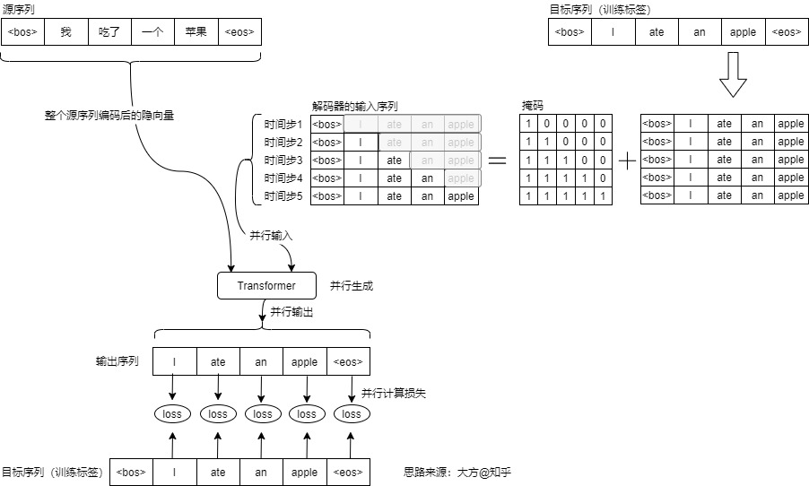
The figure is a conceptual expansion of one matrix-shaped target input; implementations need not physically duplicate the sentence into five separate tensors. Its labels are partly Chinese, and it does not distinguish structural visibility, padding validity, and loss validity as separate masks. The trace below makes those contracts explicit.

For a padded batch represented by one complete target tensor,

full_target[0] = [BOS,  8, 13, 21, EOS, PAD]
full_target[1] = [BOS,  4,  7,  9,  11, EOS]

the ordinary slicing contract is

decoder_input = full_target[:, :-1]
labels        = full_target[:, 1:]
label_valid   = labels != PAD

structural = lower_triangle(T)                       # [T,T]
key_valid  = decoder_input != PAD                    # [B,T]
read_mask  = structural[None, :, :] & key_valid[:, None, :]

which yields

decoder_input[0] = [BOS, 8, 13, 21, EOS]
labels[0]        = [8, 13, 21, EOS, PAD]
loss rows         = [1,  1,  1,   1,   0]

decoder_input[1] = [BOS, 4, 7, 9, 11]
labels[1]        = [4, 7, 9, 11, EOS]
loss rows         = [1, 1, 1,  1,   1]

The first sample still computes a final decoder row whose input is EOS, but its label is padding, so that row contributes no next-token loss. Input-key validity and prediction-row validity happen to have the same shape [B,T]; they do not have the same meaning.

0x0B.3 Training Evaluates Many Legal Prediction Rows, Not Future Decisions

All entries of decoder_input are known before the forward starts, so a Transformer can materialize hidden states

$$H^{\mathrm{train}}\in\mathbb{R}^{B\times T\times d}$$

and vocabulary logits

$$L^{\mathrm{train}}\in\mathbb{R}^{B\times T\times V}$$

for every causally legal prediction row in one tensor program. For the fixture above, B=2, T=5, and nine of ten logit rows are supervised. This is parallel evaluation of known conditional prefixes. It is not parallel discovery of y_1,\ldots,y_T.

The logits do not feed their selected IDs into later rows during the same teacher-forced forward. Row t+1 receives the gold y_t from the dataset, whether or not row t would have selected that token. This gives efficient, stable maximum-likelihood training but creates the familiar difference between gold-prefix training and model-prefix generation. Scheduled sampling, free-running objectives, and sequence-level training change that data contract; they are alternatives, not hidden steps in standard teacher forcing. M3.9 compares those training procedures and explains the consequences of training on gold prefixes but generating from model-produced prefixes.

0x0B.4 Prefill Also Has Many Known Rows, But No Training Labels

During prompt prefill, the input tokens came from the request rather than a gold target. They are nevertheless all known when the call begins. For

prompt[0] = [BOS, 5, 8, PAD, PAD]  valid length = 3
prompt[1] = [BOS, 3, 4,   7,   9]  valid length = 5

the model can evaluate all valid prompt rows together under causal visibility. There is no shifted label tensor, loss reduction, backward graph, or optimizer step. In an ordinary decoder-only continuation, the first new-token decision uses logits from the last valid prompt row:

request 0 -> physical row 2, not padded row 4
request 1 -> physical row 4

The distinction prevents a common shape-correct bug: indexing logits[:, -1] for a right-padded batch silently selects a padding row for shorter prompts. An implementation can left-pad, compact, bucket, or carry explicit sequence lengths; the invariant is semantic, not a mandate for one padding layout.

0x0B.5 Decode Exposes One New Decision Per Request And Iteration

Let request b have prompt length P_b. Index continuation decisions by r, with r=0 denoting the first decision made from prefill’s output. Later decisions follow subsequent decode forwards. Immediately before decision r, the known length is

$$K_{b,r}=P_b+r$$

provided the request remains active. This is an output-prefix length, not a count of already-materialized K/V rows. The runtime computes the distribution for the next position, the decoding policy selects one ID, and only then does that ID become a known input for iteration r+1:

known prefix at r
    -> model state for next position
        -> vocabulary scores
            -> selection policy
                -> one selected ID
                    -> append / commit
                        -> known prefix at r + 1

With the two prompts above and three synthetic selections,

iteration 0: known lengths [3,5] -> select [12, 6]
iteration 1: known lengths [4,6] -> select [15,10]
iteration 2: known lengths [5,7] -> select [EOS,EOS]

the batch produces two decisions per iteration, but still only one new future decision per request. Continuous batching can run many requests together; it does not reveal several unknown future tokens inside one request. M7 later introduces explicit draft-and-verify mechanisms that can change the number of accepted tokens per target-model iteration.

“One decision” also does not force one universal tensor extent. A naive uncached implementation can reprocess the full prefix. An incremental implementation can supply one current row while reading retained history. Both implement the same autoregressive dependency. M3.10 derives their state and equivalence contracts; M5 derives the cache and scheduler costs.

The same causal family admits different call shapes because the rows available at call start differ. The visual counts decisions, not kernel launches, and does not specify a cache layout.

0x0B.6 Encoder-Decoder Adds A Source-Memory Lifetime

For ordinary encoder-decoder generation, all valid source rows are supplied and encoded once:

source IDs [B,S]
    -> source memory [B,S,d]       retained across target iterations

target prefix [B,T_r]
    -> target hidden [B,T_r,d]     one new decision after each iteration

Cross-attention lets each legal target query read valid source-memory rows, but it does not make future target rows known. Decoder-only and encoder-decoder models can therefore share the same target-side row-availability rule while having different persistent state topologies. Re-encoding a fixed source every target step can be correct but wasteful; mutating source memory as though it were generated target state changes the program.

0x0B.7 Alternatives Change A Specific Contract

Design choice	What changes	What does not automatically change
Teacher forcing	target inputs come from shifted gold tokens	causal target visibility and autoregressive factorization
Free-running training	later training inputs can come from model decisions	sequential discovery cost and objective semantics must be declared
Scheduled sampling	mixes gold and model-provided histories under a schedule	it is not ordinary maximum-likelihood teacher forcing
Full-prefix recomputation	decode call may contain the complete known prefix	one new decision per request per iteration
Incremental execution	current input extent can shrink while history is retained	the readable history and position semantics
Batched serving	many requests share a model invocation	decisions within one ordinary request remain autoregressive

This table is a comparison by changed contract, not a recommendation. Training quality, cache bandwidth, selection policy, and serving throughput require the later articles’ objectives and measurements.

0x0B.8 Diagnosing Phase Confusions

Symptom	Shape-correct mistake	Violated invariant
Suspiciously low training loss	labels are not shifted, or row t can read y_t	the supervised token must not be visible at its own prediction row
Short prompts generate from padding	use physical final tensor row rather than last valid row	prefill decision belongs to the last valid prompt row
Training described as parallel generation	count simultaneous logit rows as discovered target tokens	gold rows were already supplied by the dataset
Prefill described as one-token decode	infer call extent from causal architecture alone	all supplied prompt rows are known together
Batched decode called multi-token generation	count one decision from each request as several future decisions for one request	request axis and future-token axis are different
Incorrect encoder-decoder state mutation	append target decisions to source memory	source memory and generated target prefix have different owners
Cache claims inferred from the architecture	assume a specific retained tensor layout from the factorization	caching is an implementation contract, not a consequence of notation alone

The decisive diagnostic is always: which rows existed before this call, which rows were legal to read, and which IDs became known only after selection?

0x0B.9 Following The Complete Execution Loops

The three phases can now be summarized by what is known before and after each call:

training:
    shifted target rows known -> many legal prediction rows -> loss/backward

prefill:
    supplied prompt rows known -> many causal rows -> first continuation decision

decode:
    generated prefix known -> one new decision per active request -> append

Use M3.9 — Training Execution for batch construction, four mask roles, loss normalization, backward, accumulation, optimizer state, dropout, exposure bias, and training variants. Use M3.10 — Single-Request Inference Execution for last-valid-row selection, prefill/decode state, stopping, cache equivalence, and commit semantics. M5 develops production cache placement, batching, and scheduling. M7 examines speculative and multi-token methods that deliberately modify ordinary decode-step accounting.

0x0C Alternative Information Paths And Multimodal Inputs

Dense attention is one answer to a routing problem, not the endpoint of sequence modeling. Once the Transformer exposes every legal token pair, later designs can ask which part of that interface is actually needed: direct random access to old rows, a fixed local graph, a compact evolving state, or several paths composed inside one block.

This raises a practical question:

When recurrence, convolution, sparse attention, structured state space, and hybrid blocks all map a sequence to a sequence, which state, graph, training schedule, and runtime contract does each mechanism actually expose?

This section compares those contracts. It does not rank model quality and it does not infer accelerator speed from an asymptotic expression.

0x0C.1 Compare State, Graph, Schedule, And Runtime Separately

The earlier sections derived recurrence, convolution, and dense attention in detail. Four coordinates keep the remaining alternatives comparable:

Coordinate	Question
exposed state	Does the next computation retain all prior rows, a bounded latent state, or both?
communication graph	Can row $i$ read row $j$ directly, only through neighbors, or only through a carried state?
known-sequence schedule	Can all supplied rows be evaluated together, and by what scan, convolution, or sparse-pair algorithm?
incremental runtime state	What must survive after one new row: K/V rows, a recurrent state, local buffers, or several owners?

Two implementations can have the same input and output shape while differing on all four coordinates. Conversely, one mathematical layer can admit two execution schedules, as the state-space derivation below demonstrates.

Reconstructed contract view. Arrows describe legal information paths, not learned importance. Runtime rows name logical retained state, not one mandatory kernel layout.

0x0C.2 Sparse Attention Removes Edges From The Pair Graph

Let $\mathcal{N}(i)$ be the key rows visible to query row $i$. Dense attention uses every legal pair; sparse attention evaluates only

$$\mathcal{E}=\{(i,j):j\in\mathcal{N}(i)\}.$$

For a bidirectional sliding window with radius $r$,

$$\mathcal{N}(i)= \{j:\max(0,i-r)\le j\le \min(T-1,i+r)\},$$

so the exact edge count is

$$|\mathcal{E}|= \sum_{i=0}^{T-1} \left[\min(T-1,i+r)-\max(0,i-r)+1\right] \le T(2r+1).$$

This replaces dense $O(T^2d)$ pair work with an $O(|\mathcal{E}|d)$ pair term. It does not provide a free global path. After $L$ contiguous-window layers, a row can move at most $Lr$ positions through those local edges before boundary effects. Dilation increases the stride of that route; designated global rows create shortcuts; neither is equivalent to simply deleting pairs.

Longformer is a concrete paper contract: it combines sliding-window self-attention with task-motivated global rows. A global row reads all sequence rows and all sequence rows can read it. The paper’s linear sequence-length claim assumes that the window and number of global rows remain bounded as $T$ grows. Its implementation discussion also matters: a sparse graph still needs a sparse/banded kernel that realizes the saved work.

This mechanism is not Luong local attention from Section 0x04. Luong local-p predicts a source-alignment neighborhood for one decoder query. Sliding-window self-attention fixes or configures legal same-sequence neighbors for every query row. Both restrict a read, but they restrict different axes under different ownership contracts.

0x0C.3 S4: One Linear State System, Two Execution Schedules

A continuous linear state-space model starts with a latent state $x(t)$, input $u(t)$, and output $y(t)$:

$$x'(t)=Ax(t)+Bu(t), \qquad y(t)=Cx(t)+Du(t).$$

Discretizing at step size $\Delta$ produces matrices $\bar A$ and $\bar B$. Under the bilinear discretization used in the S4 paper,

$$\bar A=(I-\tfrac{\Delta}{2}A)^{-1}(I+\tfrac{\Delta}{2}A), \qquad \bar B=(I-\tfrac{\Delta}{2}A)^{-1}\Delta B.$$

The discrete layer can then run as a recurrence:

$$x_k=\bar A x_{k-1}+\bar B u_k, \qquad y_k=Cx_k+Du_k.$$

With $x_{-1}=0$, substitute the state equation into itself:

$$x_k=\sum_{j=0}^{k}\bar A^{k-j}\bar B u_j,$$

and therefore

$$y_k=Du_k+ \sum_{j=0}^{k}C\bar A^{k-j}\bar B u_j.$$

Define the lag-$\ell$ kernel

$$K_\ell=C\bar A^\ell\bar B.$$

Then the same time-invariant state system is a causal convolution:

$$y=K*u+Du.$$

That equality explains the schedule change. Incremental execution can retain $x_k$ and take one recurrent step. Training on a known sequence can construct the global kernel and use convolution. The hard part is not noticing the identity; it is computing the long kernel stably and efficiently. S4’s structured parameterization of $A$ reduces that problem to tractable structured linear algebra, including a Cauchy-kernel computation. (S4)

For a batched multi-channel layer, a useful logical trace is:

known-sequence input:       u [B, T, D]
logical recurrent state:   x [B, D, N]
convolution kernel:         K [D, T]
sequence output:            y [B, T, D]

training schedule:
    parameters -> K -> causal convolution over T supplied rows

incremental schedule:
    previous x + current u_k -> new x -> current y_k

$N$ is latent state width per channel. S4 is therefore not the fixed-context encoder-decoder from Section 0x02 under a new name: it is a structured linear state transformation embedded in a deep nonlinear sequence network, with recurrent and convolutional representations of the same layer.

0x0C.4 Mamba Makes The State Update Selective

The convolutional identity above depends on time invariance: the same $\bar A$, $\bar B$, and $C$ apply at every row, so one fixed lag kernel exists. Mamba changes exactly that contract. In the paper’s selective SSM, $B_t$, $C_t$, and step size $\Delta_t$ are functions of the input; the structured $A$ remains a learned parameter. Schematically,

$$x_t=\bar A_t x_{t-1}+\bar B_t u_t, \qquad y_t=C_t x_t,$$

where discretization makes $\bar A_t$ and $\bar B_t$ depend on $\Delta_t$ and $B_t$. A fixed kernel $K_\ell$ can no longer describe every location because the transition and read coefficients vary with content.

The paper’s tensor contract makes the difference visible:

input                       u       [B, T, D]
structured parameter       A       [D, N]
input-dependent write      B_t     [B, T, N]
input-dependent read       C_t     [B, T, N]
input-dependent step       Delta_t [B, T, D]
discretized scan terms              [B, T, D, N]
output                      y       [B, T, D]

A pedagogical forward path is:

def selective_ssm(u, A, project_B, project_C, project_delta):
    B_t = project_B(u)                 # [B, T, N]
    C_t = project_C(u)                 # [B, T, N]
    delta_t = softplus(project_delta(u))  # [B, T, D]
    A_t, Bbar_t = discretize(A, B_t, delta_t)

    # A fused parallel scan evaluates supplied rows without storing
    # every expanded [B, T, D, N] state in slow memory.
    return selective_scan(A_t, Bbar_t, C_t, u)

The scan is still a recurrence algebraically. Mamba’s systems contribution is a hardware-aware parallel scan with fusion and backward recomputation, not a claim that the loop-carried dependency vanished. At incremental inference, a compact recurrent state is natural; during training, the selective scan evaluates the supplied sequence in parallel without recovering one fixed convolution kernel. (Mamba)

This is content-dependent state selection, not explicit random access to a stored list of old rows. Attention asks which prior payload rows to mix for the current query. A selective SSM asks how the current input should update and read a compressed evolving state. Those are different retrieval contracts.

0x0C.5 Hybrid Blocks Compose Paths Rather Than Choosing One Winner

Local filtering and global routing can solve different subproblems, so a model can compose them. The composition itself is a design choice:

Hybrid pattern	Computation graph	State consequence
serial sublayers	global route, then local filter, or the reverse	each sublayer consumes the previous result; ordering matters
parallel branches	local and global branches read the same input, then merge	branch outputs and merge rule need explicit owners
layer interleaving	different layer types alternate through depth	runtime state depends on which layers retain history

Conformer provides a paper-level serial example. Its block places self-attention and a convolution module between two half-step feed-forward residual updates:

$$\begin{aligned} \tilde x_i &= x_i+\tfrac12\operatorname{FFN}(x_i),\\ x'_i &= \tilde x_i+\operatorname{MHSA}(\tilde x_i),\\ x''_i &= x'_i+\operatorname{Conv}(x'_i),\\ y_i &= \operatorname{LayerNorm} \left(x''_i+\tfrac12\operatorname{FFN}(x''_i)\right). \end{aligned}$$

The attention path supplies global content interaction; the depthwise convolution module supplies local sequence structure. The paper also compares serial ordering with a parallel attention/convolution branch, which is evidence that “hybrid” does not name one canonical graph. Its results are source-reported, not reproduced here.

0x0C.6 Paper Variants By Contract

Paper mechanism	Direct token-pair read?	Known-sequence path	Incremental retained state	Contract changed
Longformer sliding + global attention	only legal sparse pairs; global rows add shortcuts	sparse/banded attention kernel	configuration-dependent; the bidirectional encoder is not an append-only causal cache	pair graph
S4	no explicit token-pair score matrix	time-invariant global convolution	recurrent latent state	structured linear state and dual schedule
Mamba selective SSM	no explicit token-pair score matrix	hardware-aware selective scan	selective recurrent state	input-dependent write/read/step
Conformer	yes, inside MHSA, plus a local convolution route	serial attention and convolution sublayers	depends on the attention/runtime architecture around the encoder	within-block route composition

The table is not a speed leaderboard. O(Tw), near-linear S4 kernel construction, and linear-work selective scans are algorithmic contracts. Wall time additionally depends on layout, fusion, memory traffic, sequence length, batch shape, and available kernels.

0x0C.7 Show, Attend And Tell: Visual Memory Before Modern MLLMs

The translation alignment pressure also appeared in image captioning. Show, Attend and Tell uses a convolutional encoder to produce $L$ annotation vectors, each tied to an image location:

$$a=\{a_1,\ldots,a_L\}, \qquad a_i\in\mathbb{R}^{D_v}.$$

At caption step $t$, an MLP scores each annotation using the previous LSTM hidden state:

$$e_{t,i}=f_{\mathrm{att}}(a_i,h_{t-1}), \qquad \alpha_{t,i}=\frac{\exp(e_{t,i})} {\sum_{j=1}^{L}\exp(e_{t,j})}.$$

The deterministic soft variant reads the expected visual annotation:

$$\hat z_t=\sum_{i=1}^{L}\alpha_{t,i}a_i.$$

Its tensor trace is the same alignment contraction from translation with a different memory owner:

visual annotations       A         [B, L, D_v]
previous decoder state   h_(t-1)   [B, H]
location scores          e_t       [B, L]
source-axis weights      alpha_t   [B, L]
visual context           z_t       [B, D_v]
next-word distribution             [B, V]

The paper also studies a stochastic hard variant. A one-hot latent location $s_t$ is sampled from the categorical distribution parameterized by $\alpha_t$, so $\hat z_t=\sum_i s_{t,i}a_i$. Because that sample is discrete, ordinary pathwise backpropagation cannot differentiate through the sampled location. Marginalizing every attention trajectory would give

$$p(y\mid a)=\sum_s p(s\mid a)p(y\mid s,a).$$

Jensen’s inequality produces the paper’s lower-bound objective:

$$\log p(y\mid a) \ge \mathbb{E}_{s\sim p(s\mid a)} \left[\log p(y\mid s,a)\right] =\mathcal{L}_s.$$

Its gradient contains a score-function term:

$$\mathbb{E}_{s\sim p(s\mid a)} \left[ \log p(y\mid s,a)\nabla\log p(s\mid a) \right],$$

which the paper estimates with Monte Carlo samples and variance-reduction devices; this is the REINFORCE form. The soft variant replaces the sampled location with the expected annotation and uses ordinary backpropagation. These are different training contracts, not two drawing styles for the same operation. (Show, Attend and Tell)

Reconstructed historical bridge. The visual states are encoder annotations, not text token IDs, and an attention heat map records model weights rather than proving a causal explanation.

The analogy is precise but bounded:

translation:
    target state -> weights over source-text states -> linguistic context

image captioning:
    caption state -> weights over spatial image annotations -> visual context

The external memory owner changes. The weighted-read interface survives.

0x0C.8 From Visual Features To A Multimodal Model

The weighted-read interface carries across modalities, but raw images still need to become usable model inputs. Matching vector widths makes tensors compatible; learning useful relationships between their representations requires encoders, fusion, and training. The X1 chapters develop that path:

• X1.1 — Unitization, Geometry, And Metadata explains pixels, patches, regions, tiles, coordinates, validity, origin maps, and processor-manifest compatibility;
• X1.2 — Encoders, Projectors, And Fusion develops modality encoders, layer selection, width projectors, prefix fusion, cross-attention, learned-query bottlenecks, and paper-specific training stages;
• X1.3 — Masks, Training, And Runtime State examines placeholder expansion, mixed-origin packing, visibility and loss masks, multimodal training rows, prefill/decode state, caching, batching, and safe release.

Together, these steps explain how visual evidence enters a sequence model and remains identifiable through training and generation.

0x0C.9 Distinctions That Matter In Practice

Failure	What went wrong	Required correction
S4 described as an ordinary RNN	recurrence representation was mistaken for the whole structured layer	preserve the continuous, recurrent, convolutional, and structured-kernel views
Mamba described as a fixed convolution	input-dependent $B_t$, $C_t$, and $\Delta_t$ were erased	use the time-varying selective-scan contract
sparse attention equated with Luong local-p	same-sequence graph sparsity was confused with decoder-to-source alignment	name query owner, key owner, and neighborhood rule
algorithmic linear work called hardware speed	graph work was treated as a benchmark	measure kernels, traffic, shapes, and hardware before a runtime claim
visual annotations called token IDs	encoder feature rows were confused with discrete vocabulary symbols	preserve modality, geometry, and origin metadata; continue in X1.1
attention heat map called causal explanation	visible weights were promoted beyond their evidence	treat the map as model behavior unless a stronger causal analysis is performed
equal widths called modality alignment	shape compatibility was confused with learned semantic compatibility	continue with projectors and training contracts in X1.2

0x0C.10 Checking A Complete Sequence Model

Several mistakes survive ordinary shape checks because they change the meaning of a tensor or operation without changing its dimensions. The following checks connect the distinctions developed throughout the article.

Mistake	Why a shape check can miss it	Invariant	What to inspect
multiple attention hops mislabeled as Transformer multi-head attention	both produce several weighted summaries	a hop changes the number of pooling rows; a Transformer head owns projected Q/K/V subspaces plus concatenate-and-fuse semantics	pooling rows versus projected heads and output fusion
decoder self-attention and cross-attention accidentally tied	both modules can have the same hidden width and attention class	semantic role identity must remain distinct unless tying is an explicit architecture choice	distinct module references, parameter objects, and mutation isolation
source and target masks swapped with shape-compatible lengths	equal padded extents permit broadcasting and indexing	every mask carries query owner, key owner, and visibility relation, not shape alone	query stream, key stream, and the resulting read relation
hidden state sampled as if it were logits	hidden and vocabulary widths can coincide in a toy or tied setup	selection consumes generator logits or probabilities; it does not consume an arbitrary hidden state	vocabulary projection and the axis used for selection
attention weights presented as a causal explanation	a normalized heat map is easy to display and interpret	weights are model behavior unless a separate causal or counterfactual analysis supports a stronger claim	whether causal or counterfactual evidence supports the interpretation
decoder-only described as always one-token input	causal visibility is present in training, prefill, and decode	architecture fixes legal visibility; execution phase fixes how many supplied rows are known	rows supplied before the call versus IDs selected afterward
training labels exposed as legal attention inputs	labels and decoder inputs have aligned sequence extents	shifting and causality keep the same-row label outside the legal input prefix	shifted inputs, labels, read masks, and loss-validity rows

The accompanying examples reproduce small construction and tensor checks; they do not train a Transformer or measure its quality. The example command in 0x0A.6 provides one way to test the difference between equal dimensions and interchangeable state.

The durable conclusion is narrower than “attention won” and more useful:

Choose the state, graph, schedule, and runtime ownership needed by the task. Then verify that the implementation realizes that contract rather than only sharing its input and output shape.

0x0D Summary

The purpose of the historical comparison was to understand design choices that remain visible in a running model. Translation gave us a concrete task:

source sequence -> target sequence

The conditional chain rule describes a probability for the output sequence; it does not choose the neural architecture that evaluates each factor. A fixed-context encoder-decoder represents the source with one summary. Attention changes that interface by retaining source states and constructing a different weighted read for each target step.

Recurrence gives the model a shared transition across time:

h_t = f(x_t, h_{t-1})

Gates can improve what the state carries, but the next state still depends on the previous one. Convolution makes known positions within a layer parallelizable, at the cost of a neighborhood determined by kernel geometry and a receptive field that depends on depth. Neither choice is simply obsolete: each provides useful biases and different state requirements.

Residual connections address depth rather than source selection:

$$y = x + F(x)$$

They provide an identity route alongside a learned update. Attention addresses a different question: which available states should contribute to the current computation? In an attentional translation model, the read is

decoder state
    -> attention over encoder states
    -> step-dependent context vector

and in self-attention it becomes

sequence positions
    -> self-attention over other sequence positions
    -> contextualized token states

The Transformer combines these content-dependent reads with position information, row-wise transformations, normalization, and residual depth. Encoder-only, decoder-only, and encoder-decoder models arrange these operations differently. Their visibility rules determine which rows may interact, but their output heads and training objectives must still be specified.

The implementation brings these distinctions together:

text -> tokens -> IDs -> initial state -> contextual state -> logits -> selected IDs

That is the path for vocabulary-based generation, not the only possible readout. Module objects hold parameters; runtime tensors carry a particular input. Training compares predictions with labels and updates parameters. Prefill processes a supplied prompt. Subsequent ordinary decode steps use the growing prefix to make further decisions. The same weights therefore participate in different programs.

We can now ask more useful questions than whether a model “uses attention.” Which states are available? Which may be read? What does the returned tensor mean? What must remain between calls? Those questions connect an architectural choice to a correct implementation, and a correct implementation to the training and runtime costs we will investigate throughout Transformer System.

The historical notes below provide a closer comparison of the papers and their terminology. For the next step into the input path, continue with tokenization and sequence preparation.

0x0E Historical Notes: Related Ideas, Different Mechanisms

The arrows organize interface pressure. A dotted arrow is explicitly not a claim that one paper caused, copied, or had priority over the next. The tables below distinguish the publication dates and mechanisms behind the nodes.

The mechanisms in this article developed along overlapping lines. Reading the history after the tensor examples makes several distinctions easier to see: Lin et al.’s attention hops are not Transformer heads; Daniluk et al.’s recurrent key-value memory is not a parallel Q/K/V layer; residual connections change paths through depth rather than paths between sequence positions.

0x0E.1 Publication Dates And Overlapping Developments

A history can become misleading before it reaches the mechanism. An arXiv submission month and a conference proceedings date are different coordinates. This article uses the proceedings date by default. When the arXiv version materially predates the proceedings or helps separate several 2017 papers, both coordinates are printed. For example, Bahdanau et al. is labeled arXiv September 2014 / ICLR 2015, while Luong et al. is labeled EMNLP September 2015. The former is not silently moved after every 2014 conference paper just because its proceedings appeared in 2015.

The map is also deliberately selective. It does not claim to identify the first use of every word, nor does it turn citations into a clean family tree. It asks a narrower engineering question at every node:

what state existed before the paper?
    -> which interface did the paper change?
    -> what pressure remained after that change?
    -> which later term must not be substituted for the paper's own mechanism?

That contract produces three overlapping threads: source-to-target transduction, same-stream content addressing, and deep optimization. The Transformer combines parts of all three, but the threads did not wait for one another in a single queue.

0x0E.2 Sequence Transduction: From Conditioning To Addressable Source State

The first thread is about the boundary between a source sequence and a target generator. Its central change is not “RNN became attention.” The boundary first became differentiable, then end-to-end, then addressable at each target step, and finally compatible with parallel source-state construction.

Publication coordinate	Paper contract	Interface change	Pressure that remains
EMNLP Oct 2013	Recurrent Continuous Translation Models	A recurrent target language model is conditioned by continuous source representations produced by convolutional source models.	Source-target relations are learned implicitly; there is no learned per-target soft alignment over source annotations.
EMNLP Oct 2014	Cho et al., RNN Encoder-Decoder	One RNN maps a variable-length phrase to a fixed-length vector; a second RNN maps that vector to a variable-length target phrase; the neural pair is trained jointly.	The source still crosses one fixed vector. In the reported SMT experiment, the neural phrase score is an additional feature in a larger log-linear system.
NIPS 2014	Sutskever et al., Sequence to Sequence Learning	A deep LSTM encodes the entire source into a fixed-dimensional representation and a second deep LSTM directly generates the target sequence.	End-to-end generation removes the phrase-table deployment boundary, but not the fixed-vector source bottleneck or recurrent critical path.
arXiv Sep 2014 / ICLR 2015	Bahdanau et al., Jointly Learning to Align and Translate	The decoder receives an addressable set of encoder annotations and constructs a different weighted source context at each target step.	Dynamic retrieval changes source access, but the encoder and decoder still update through recurrent chains.
EMNLP Sep 2015	Luong et al., Effective Approaches to Attention	Global versus local source windows and dot, general, and concat score functions become explicit design choices.	Attention is configurable retrieval attached to a recurrent translation model, not yet the main sequence-state update.
arXiv May 2017 / ICML Aug 2017	Gehring et al., Convolutional Sequence to Sequence Learning	Convolutional stacks make position updates parallel during training; each decoder layer has its own source-attention module.	Long-range interaction through the convolutional path still grows with depth, and autoregressive target generation remains sequential.
arXiv Jun 2017 / NIPS Dec 2017	Vaswani et al., Attention Is All You Need	Projected self-attention and cross-attention become the principal sequence-interaction operations inside residual, normalized, position-wise feed-forward stacks.	Full score matrices introduce pairwise sequence work and memory; M4 and M5 later account for those costs and persistent states.

RCTM should not be confused with the later all-recurrent encoder-decoder. The RCTM paper defines

$$p(f\mid e)=\prod_{i=1}^{m}p(f_i\mid f_{<i},e),$$

but its source conditioning is convolutional and its target generator is a recurrent language model. In RCTM I, a convolutional sentence model produces a source representation that conditions each target hidden update. RCTM II uses a more local source-to-target representation path. This is an important early continuous conditional translation contract, but calling it the Cho-style RNN encoder-decoder erases the actual source computation.

Cho et al. then make the fixed-vector interface explicit:

x_1 ... x_T
    -> recurrent encoder
    -> c = final source summary
    -> recurrent decoder conditioned on c
    -> p(y_t | y_<t, c)

The encoder and decoder are jointly differentiable and jointly trained. The full reported translation pipeline, however, is not only that pair: the model scores phrase pairs and contributes those probabilities to a conventional SMT log-linear model. “Jointly trained neural encoder-decoder” and “end-to-end deployed neural translation system” are therefore separate claims.

Sutskever et al. remove that deployment boundary by having the second LSTM generate the translation directly. Their source reversal trick shortens useful optimization paths in the dataset, and LSTM gating improves recurrent credit assignment, but neither changes the cardinality of the source interface: many source rows still become one fixed-dimensional vector. The paper is a decisive end-to-end sequence-learning contract, not the disappearance of compression.

Bahdanau attention changes that cardinality. Let encoder annotations be $h_1,\ldots,h_{T_x}$ and let $s_{i-1}$ be the previous target-side state. A compatibility network produces

$$e_{i,j}=a(s_{i-1},h_j), \qquad \alpha_{i,j}=\frac{\exp(e_{i,j})}{\sum_{k=1}^{T_x}\exp(e_{i,k})}, \qquad c_i=\sum_{j=1}^{T_x}\alpha_{i,j}h_j.$$

The key historical change is not only the weighted sum. It is that the decoder can construct a new source read $c_i$ for each target position instead of receiving the same $c$ at every step. Luong et al. then expose two more design axes: what may be scored (all source states or a local window) and how it is scored (dot, learned bilinear/general, or concat-style compatibility). Their formulation also uses the current decoder hidden state in the attention path, while the Bahdanau formulation above uses the previous target state in its alignment model. The label “attention” therefore does not fix state timing, score function, or candidate memory.

ConvS2S changes a different part of the critical path. Convolutions allow the training-time state update for all positions in a layer to execute in parallel, and stacking expands the receptive field. Its multi-step attention means that source attention is applied at multiple decoder layers. It does not mean that one attention layer has multiple projected heads. That distinction matters when this history reaches the Transformer.

0x0E.3 Residual Depth And Same-Stream Addressing

Attention did not by itself explain how to train a deep stack. He et al.’s residual learning changes a block from learning a complete replacement state to learning a residual update around an identity path:

$$x_{\ell+1}=x_{\ell}+F_{\ell}(x_{\ell}).$$

The path is architectural, not attentional. It preserves a route for state and gradients through a deep composition. The Transformer adopts residual connections around attention and feed-forward sublayers, but residual learning does not determine which positions may interact.

A second side thread moves attention inside one sequence or memory stream:

Publication coordinate	Paper contract	Exact terminology boundary
arXiv Jan 2016 / EMNLP Nov 2016	Cheng et al., Long Short-Term Memory-Networks for Machine Reading preserve hidden and memory tapes and use intra-attention to address previous token states inside the recurrent update.	Same-sequence access does not imply a parallel Transformer self-attention layer; the controller still advances recurrently.
arXiv Feb 2017 / ICLR 2017	Daniluk et al., Frustratingly Short Attention Spans separate recurrent outputs into key, value, and prediction representations for a sliding-window memory.	This is key-value-predict memory, not a Transformer query/key/value projection pipeline and not multi-head attention.
arXiv Mar 2017 / ICLR 2017	Lin et al., A Structured Self-Attentive Sentence Embedding use multiple attention hops to produce a matrix sentence embedding from BiLSTM states.	A hop is a row of sentence-pooling weights. It is not a learned Q/K/V head followed by concatenation and an output projection.

The LSTMN makes recurrence less aggressively compressive by retaining two tapes, $H_{t-1}=(h_1,\ldots,h_{t-1})$ and $C_{t-1}=(c_1,\ldots,c_{t-1})$. The current input and previous summary score the hidden tape; the resulting weights retrieve adaptive summaries from both tapes before the new recurrent state is written. This is a genuine same-sequence attention relation, but attention remains a subroutine inside a left-to-right state machine.

Daniluk et al. address role overload rather than recurrence itself. A baseline memory-augmented language model uses one recurrent output for next-token prediction, attention addressing, and memory content. Their variants separate that output into

$$h_t=[k_t;v_t] \quad\text{or}\quad h_t=[k_t;v_t;p_t],$$

so keys determine memory weights, values supply retrieved content, and $p_t$ encodes the next-word distribution in the key-value-predict variant. The paper does not define the Transformer pattern $Q=XW_Q$, $K=XW_K$, $V=XW_V$ over a whole state matrix. Calling it “the first QKV attention” would therefore assert a tensor contract that the paper does not have.

Lin et al. use a BiLSTM state matrix $H$ and compute

$$A=\operatorname{softmax}\!\left(W_{s2}\tanh(W_{s1}H^\mathsf{T})\right), \qquad M=AH.$$

If $A\in\mathbb{R}^{r\times T}$, its $r$ rows are attention hops and $M\in\mathbb{R}^{r\times 2u}$ is a matrix sentence embedding. The rows are encouraged to attend to different sentence aspects through a diversity penalty. Transformer heads instead project per-position states into several Q/K/V subspaces, perform several attention operations, concatenate per-position outputs, and apply an output projection. Similar plurality does not make the operations aliases.

0x0E.4 Similar Names, Different Computations

The following terms describe different axes. Substituting one for another is a mechanism error, not merely a naming preference.

Term	Contract in this article	Do not silently replace it with
Sequence-to-sequence	A variable-length sequence mapping task family.	Only Sutskever et al.’s fixed-vector LSTM implementation.
Encoder-decoder	A source representation path plus a target generation path.	An RNN-only architecture, attention, or a fully neural deployed pipeline.
Fixed context	One source summary $c$ reused across target steps.	A target-step context $c_i$ recomputed by alignment.
Alignment attention	A target-side state scores source annotations.	Same-stream self-attention.
Self- or intra-attention	Querying and addressed state belong to the same sequence or memory stream.	Automatic Transformer-style parallelism or multi-head projection.
Key-value separation	Address representations and retrieved payload representations are distinct.	The complete Transformer Q/K/V score path.
Multiple attention hops	Multiple rows of pooling weights produce multiple sentence vectors.	Multi-head attention.
Multi-step attention	Attention is repeated at multiple decoder layers or recurrent steps.	Several parallel heads inside one attention layer.
Multi-head attention	Several learned Q/K/V projection subspaces compute attention in parallel, concatenate, and fuse through an output projection.	Multiple hops, repeated attention, or key-value memory alone.
Residual connection	An identity state path plus a learned residual update.	An attention or routing rule.

The shortest correct interface trace is therefore:

fixed source interface:
    source rows -> one c -> every target step reads the same c

alignment interface:
    source rows -> H
    target state s_i + H -> alpha_i -> target-specific c_i

same-stream memory interface:
    current recurrent state + prior-state tape -> weights -> retrieved prior content

Transformer interface:
    state matrix X -> projected Q, K, V
    Q K^T -> per-row normalized weights -> per-row value mixture
    several projected heads -> concatenate -> output projection

These traces explain why “hop,” “step,” “key-value,” and “head” cannot be substituted for one another. For the projected attention calculation, continue with scaled dot-product attention and multi-head attention.

0xFF Reference

Primary Papers And Official Technical Sources

• Recurrent Continuous Translation Models
• Learning Phrase Representations using RNN Encoder-Decoder for Statistical Machine Translation
• Sequence to Sequence Learning with Neural Networks
• Neural Machine Translation by Jointly Learning to Align and Translate
• Effective Approaches to Attention-based Neural Machine Translation
• Long Short-Term Memory
• Learning to Forget: Continual Prediction with LSTM
• On the difficulty of training Recurrent Neural Networks
• Long Short-Term Memory-Networks for Machine Reading
• Scheduled Sampling for Sequence Prediction with Recurrent Neural Networks
• Convolutional Sequence to Sequence Learning
• WaveNet: A Generative Model for Raw Audio
• Deep Residual Learning for Image Recognition
• Frustratingly Short Attention Spans in Neural Language Modeling
• A Structured Self-Attentive Sentence Embedding
• Attention Is All You Need
• The Annotated Transformer
• BERT: Pre-training of Deep Bidirectional Transformers for Language Understanding
• Improving Language Understanding by Generative Pre-Training
• Unified Language Model Pre-training
• Exploring the Limits of Transfer Learning with a Unified Text-to-Text Transformer
• Attention is not Explanation
• Longformer: The Long-Document Transformer
• Efficiently Modeling Long Sequences with Structured State Spaces
• Mamba: Linear-Time Sequence Modeling with Selective State Spaces
• Conformer: Convolution-augmented Transformer for Speech Recognition
• Show, Attend and Tell: Neural Image Caption Generation with Visual Attention

Contextual Historical Sources

The papers above provide the technical evidence. The resources below offer additional historical discussion and visual explanations; they are not interchangeable with the cited paper’s equations or experimental conditions.

• Thang Luong’s Thesis on Neural Machine Translation
• Bahdanau and Luong Attention: An Intuitive Introduction
• Two attention mechanisms in seq2seq: figure and formula
• Understanding the Differences between Bahdanau and Luong Attention
• Transformer Bottom-up Understanding (4): Attention without RNN
• Learning Large Models Through Pictures: The Past and Present of Transformers
• Progress and Conjectures of Non-Transformer Architectures

Related Explanations And Figure Credits

• Transformer Series (1) — Attention Mechanism
• Transformer Series (2) — Overall Architecture
• Transformer Series (4) — Encoder and Decoder
• Transformer Series (5) — Training and Reasoning
• Transformer Series (10) — Self-Attention
• Transformer Series (11) — Masks
• Transformer Series (20) — KV Cache
• M3.7 — Residual Stream, Normalization, and Block Assembly
• M3.9 — Training Execution
• M3.10 — Single-Request Inference Execution
• X1.1 — Unitization, Geometry, and Metadata
• X1.2 — Encoders, Projectors, and Fusion
• X1.3 — Masks, Training, and Runtime State
• Simon J. D. Prince, Understanding Deep Learning, Chapters 10–12: convolution, residual depth, and Transformer representations.
• A Neural Probabilistic Language Model, Bengio et al., 2003: learned representations and sequence probabilities.
• LLMCad: Fast and Scalable On-device Large Language Model Inference, Xu et al.: source of the opening generation illustration.