M3.2 — Multi-Head and Cross-Attention: Projection, Layout, and Variants
M3.2 — Multi-Head and Cross-Attention: Projection, Layout, and Variants
0x00 Overview And Background
M3.1 opened one scaled dot-product attention call:
query, key, value
    -> scores
    -> mask / bias
    -> softmax
    -> p_attn @ value
That function assumes Q/K/V are already projected and head-shaped:
query: [B, h, q_len, d_head]
key:   [B, h, k_len, d_head]
value: [B, h, k_len, d_head]
M3.2 opens the caller that creates those tensors.
The local object is the Harvard MultiHeadedAttention module from
A12, reconciled against
the official Annotated Transformer:
X_q:      [B, q_len, d_model]
X_k, X_v: [B, k_len, d_model]
    -> W_Q, W_K, W_V projections
    -> split last dimension into h heads
    -> transpose to [B, h, q_len/k_len, d_k]
    -> call attention(...)
    -> transpose heads back
    -> contiguous().view(...)
    -> W_O output projection
This article is not another explanation of softmax attention. It is about the tensor layout around the attention primitive.
The original Transformer paper separates the inner scaled dot-product primitive from the outer multi-head wrapper. That distinction is the same boundary used between M3.1 and M3.2:
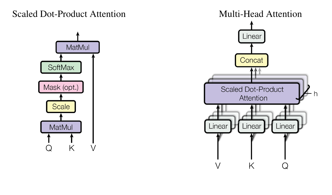
Source: Attention Is All You Need, Figure 2.
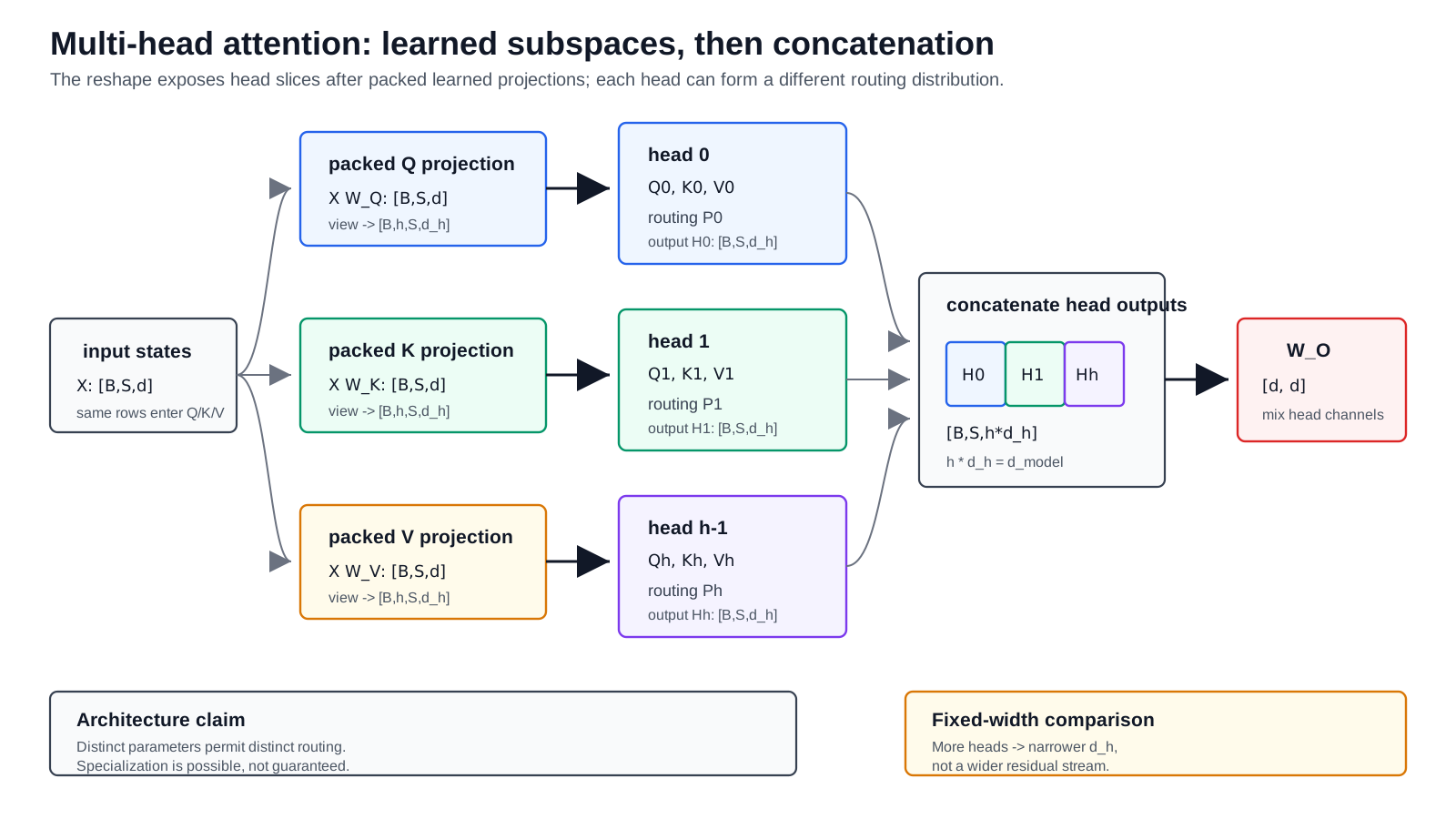
The source-series reconstruction below expands the right-hand diagram into the exact packed projection, reshape, transpose, concatenate, and output-projection path used by the Harvard implementation.
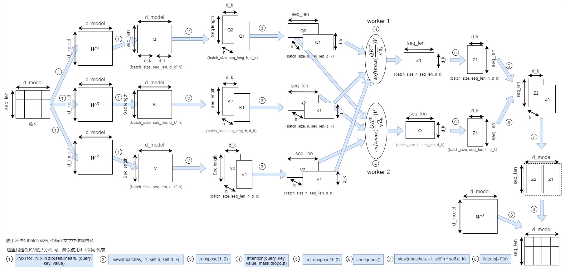
Background knowledge: several representation subspaces, one packed kernel path
Multi-head attention was introduced so the model could learn several query-key-value projections instead of forcing one similarity space to represent every relation. Conceptually, each head owns a lower-dimensional routing distribution. Implementations usually compute those heads with packed matrices rather than independent Python modules.
conceptual view:
    h learned attention subspaces

parameter view:
    large W_Q, W_K, W_V and W_O matrices

layout view:
    split d_model into h by d_head, then transpose axes

execution view:
    batched head-shaped score and value matmuls
This distinction explains why head count is both a modeling choice and a tensor-layout constraint. The module must return to [B,S,d_model] so residual and downstream block contracts remain valid.
Owner question and thesis
Owner question: How are model-width states projected into head-local Q/K/V tensors, executed through one attention primitive, merged back into the residual width, and reused when decoder queries read fixed encoder memory?
The short answer is not merely “split the hidden dimension.” Multi-head attention is simultaneously two objects:
learned object:
    several Q/K/V projection families
    -> several normalized routing distributions
    -> several value subspaces
    -> one learned output fusion

tensor program:
    packed projection matrices
    -> shape/stride transforms exposing a head axis
    -> one batched attention call
    -> transpose + contiguous materialization + merge
    -> one output projection
Those descriptions are equivalent only when the per-head equations, packed checkpoint slices, axis order, output-projection blocks, and backward paths all agree. A module can have the expected final shape and still be wrong because it mixed token and head axes, loaded a fused checkpoint in the wrong order, used source rows as decoder queries, or reused projected cross-KV from an incompatible encoder/projection release.
The thesis of M3.2 is therefore:
Multi-head attention is a learned direct-sum decomposition implemented as a packed tensor program. Cross-attention reuses that program while changing who owns Q, who owns K/V, and how long the projected source state may live.
This is why the article keeps algebra, tensor layout, checkpoint state, training, and runtime integration together. None can certify the others alone.
Historical pressure: one routing distribution is one bottleneck
The chronology here is selective. M1.1 owns the longer path from recurrent fixed-context compression through query-conditioned alignment. M3.2 begins after the local normalized retrieval operation already exists.
For one projected attention call, suppressing batch axes, write:
For every query row, A supplies one probability distribution over the key
axis. Increasing the channel width of Q, K, and V can make that one
distribution depend on a richer representation, but it does not create a
second independently normalized routing decision. All output channels in that
call are mixed with the same row of A.
The original Transformer introduced the canonical multi-head construction by learning several lower-dimensional projection families:
The structural change is now visible. Each head has its own learned Q/K
geometry and therefore its own normalized matrix A_i. The value rows can be
read differently by each head before W_O fuses the resulting channels.
This gives the model capacity for several routing relations. It does not prove that every trained head becomes a stable linguistic module, that heads have unique meanings, or that a visualization is a causal explanation. Those claims require the evidence hierarchy developed later in this article.
Why fixed total width keeps the canonical cost comparison meaningful
A naive reading might imagine H full-width attention modules, multiplying
projection and value-mixing work by H. Canonical MHA instead divides the
model width across heads:
For a self-attention sequence of length S, the three packed projections have
the same broad matrix shapes as three full-width linear maps:
X:   [B,S,D_model]
W_Q: [D_model,H*D_qk] = [D_model,D_model]
W_K: [D_model,H*D_qk] = [D_model,D_model]
W_V: [D_model,H*D_v]  = [D_model,D_model]
The score work summed over heads is
and the value-mixing work has the same cancellation when D_v=D_model/H.
That is the precise sense in which the original fixed-width construction keeps
the broad attention arithmetic comparable to one full-width head. It does not
say every head count has identical kernel efficiency, launch overhead,
occupancy, numerical behavior, or checkpoint size. M4 prices those physical
effects after M3.2 defines the tensors.
Nor is equal width a mathematical requirement. The local attention primitive needs matching Q/K widths, while V may use a different width. Equal slices are the regular packing contract used by the canonical implementation; asymmetric and heterogeneous cases appear below because they force the hidden assumptions into the open.
Conceptual heads and packed execution are the same map under a storage contract
Conceptually, per-head projections are independent matrices:
An implementation need not launch H separate linears. It can concatenate
them by output channel:
Then
view(B,Q,H,D_qk).transpose(1,2) does not invent heads; it exposes the head
blocks already encoded in the packed output-channel order. A fused QKV matrix
adds another storage decision: whether the packed axis is organized as
[all-Q | all-K | all-V], interleaved by head, or under another documented
layout. Shape and element count cannot identify that convention.
The inverse side has the same discipline. Concatenation preserves head output
blocks, and W_O can be partitioned by its input rows:
This direct-sum form will matter for head permutations, pruning, routed heads,
and backward. It also explains why “average the heads” is not a drop-in
replacement for canonical concat-plus-W_O.
Cross-attention changes state ownership, not the local formula
Self-attention passes one state object into all three roles:
X_q = X_k = X_v = current stream
Encoder-decoder cross-attention instead passes two objects:
X_q = decoder target state: [B,T,D_model]
X_k = encoder source memory: [B,S,D_model]
X_v = encoder source memory: [B,S,D_model]
After projection, the local M3.1 primitive sees:
Q: [B,H,T,D_qk]
K: [B,H,S,D_qk]
V: [B,H,S,D_v]
A: [B,H,T,S]
O: [B,H,T,D_v]
The arithmetic remains softmax(QK^T)V, but the lifecycle changes. During
training, gradients return through decoder queries and encoder memory. During
autoregressive inference, target self-KV grows with every decoded token while
the projected encoder K/V can remain fixed and be reused by later target
queries. Beam expansion may share, expand, or index that source state, but it
must not silently change its content.
Therefore cross-KV reuse is not authorized by shape alone. It is bound to at least the source example, encoder output, layer, K/V projection parameters, adapter state, dtype/layout, and release identity. M3.2 owns that one-request state contract. M5 later owns multi-request allocation and scheduling.
Two reading lanes
The rest of M3.2 has two connected lanes:
| Lane | Question | Main objects |
|---|---|---|
| Canonical wrapper and cross-attention | How do equations become one correct packed training/runtime program? | projection/checkpoint slices, head axes, strides, W_O, gradients, source/target state, cross-KV |
| Head evidence and variants | What does a paper change, and what conclusion or efficiency claim follows? | maps, ablations, gates, overlap, head-axis transforms, dynamic composition, routing |
They stay in one article because every variant is defined relative to the
canonical head and W_O contract. The variant lane may change channel
partitioning, score/probability head composition, or active head selection; it
must still state how its output returns to the block interface.
Owner contract: consumes, owns, and defers
| Relationship | Contract |
|---|---|
| consumes from M2.2 | model-width rows and checkpoint-compatible initial state; M3.2 does not re-derive token addresses or embedding-table training |
| consumes from M3.1 | one local attention primitive over projected head-shaped Q/K/V, including score scaling, visibility, softmax, probability dropout, value mixing, and local derivatives |
| accepts from M3.3-M3.5 | positional or bias objects at declared insertion points; their geometry and extension rules remain with those articles |
| owns in M3.2 | Q/K/V projection, head split/merge, storage/checkpoint layout, W_O, wrapper backward, self/cross caller roles, fixed cross-KV lifetime, and head-composition variants |
| defers to M3.7 | residual ordering, normalization, and complete block assembly |
| defers to M4.3-M4.6 | IO-aware algorithms, fused-kernel schedules, and hardware pipeline proof |
| defers to M5.7-M5.8 | MQA/GQA shared-KV serving derivation and MLA latent-cache mechanics |
| defers to M6.1 | routed FFN capacity, expert balance, and expert-parallel communication; MoH is compared here only as attention-head routing |
| parallel handoff to X1.2 | modality encoders/projectors may produce external source memory, while this article supplies the generic target-query/source-KV contract |
This is a bottom-up reading order, not a claim that a production system runs these concerns in separate libraries. The point is to prevent one article from silently changing an object whose semantics are owned elsewhere.
Claim status and reading rules
M3.2 uses the following evidence labels:
| Label | Meaning in this article |
|---|---|
| Source-local | faithfully reconstructed from A2, A4, A10, or A12; not automatically externally verified |
| Externally verified | supported by a cited primary paper |
| Official version-scoped | supported by a pinned framework document or source revision; not universal across versions |
| Derivation | follows algebraically from declared shapes and assumptions and is checked against an executable oracle where provided |
| Rewrite interpretation | explanatory synthesis or an ownership/design recommendation |
| Source-reported | an empirical observation or benchmark retained with its paper, model, task, and intervention scope |
| Uncertain | plausible but not sufficiently verified; it must not carry a publish-critical claim |
Three rules matter especially:
- An attention map is an observed normalized weight matrix, not a causal proof of why the model produced its output.
- A paper’s nominally smaller active-head set is not a runtime speedup unless the implementation avoids the inactive work and the measurement contract is stated.
- Framework fastpath behavior is Official version-scoped. Logical tensor equivalence does not prove that two calls dispatch the same kernel.
0x01 The code spine
A12’s central code object is:
class MultiHeadedAttention(nn.Module):
    def __init__(self, h, d_model, dropout=0.1):
        "Take in model size and number of heads."
        super(MultiHeadedAttention, self).__init__()
        assert d_model % h == 0

        self.d_k = d_model // h
        self.h = h
        self.linears = clones(nn.Linear(d_model, d_model), 4)
        self.attn = None
        self.dropout = nn.Dropout(p=dropout)

    def forward(self, query, key, value, mask=None):
        if mask is not None:
            mask = mask.unsqueeze(1)

        nbatches = query.size(0)

        query, key, value = [
            lin(x).view(nbatches, -1, self.h, self.d_k).transpose(1, 2)
            for lin, x in zip(self.linears, (query, key, value))
        ]

        x, self.attn = attention(
            query, key, value, mask=mask, dropout=self.dropout
        )

        x = (
            x.transpose(1, 2)
            .contiguous()
            .view(nbatches, -1, self.h * self.d_k)
        )

        del query
        del key
        del value

        return self.linears[-1](x)
Read it as a shape machine:
query rows:
    [B,q_len,d_model]

key/value rows:
    [B,k_len,d_model]

projected rows:
    [B,q_len,d_model] and [B,k_len,d_model]

head-shaped rows:
    Q: [B,h,q_len,d_k]
    K: [B,h,k_len,d_k]
    V: [B,h,k_len,d_k]

attention output per head:
    [B,h,q_len,d_k]

merged rows:
    [B,q_len,d_model]

final output:
    [B,q_len,d_model]
The module preserves the residual-stream width. That is why the next block component can receive the same row shape.
0x01A Immutable projection and call manifest
The code spine is compact because many contracts are implicit. zip assumes
that the first three linears still mean Q, K, and V. view assumes that the
projection output was packed head-major with the expected widths. The call
site assumes that query, key, and value came from the intended model
states. A framework dispatcher assumes particular mask, dtype, dropout, and
output requirements before it admits a backend.
These assumptions are individually easy to satisfy by shape and collectively easy to violate by meaning. M3.2 therefore uses an immutable call manifest: a per-call record frozen before projection begins. Immutable here does not mean that a Python dictionary is magical. It means that the identities which define the call cannot change between validation, execution, cache reuse, and reconciliation. Its central test is whether a shape-compatible wrong-origin bundle is rejected before any projection executes.
Six identities that must not collapse into one shape
Consider a canonical tensor with shape [B,S,D]. That shape does not identify:
- semantic state — encoder source rows, decoder target rows, or a self-attention stream;
- logical projection — Q, K, V, or output;
- mathematical orientation — the article’s right-multiplication map
[D_in,D_out]; - framework storage — for example a PyTorch linear weight stored as
[D_out,D_in]; - checkpoint span — a separate tensor or an interval inside fused QKV;
- runtime object — request, layer, checkpoint release, adapter, dtype, device, and backend attempt.
A validator must therefore compare identities, not only extents. Swapping two
equal Q and K chunks in a fused self-attention checkpoint preserves every
matrix shape. Reusing projected cross-KV from another source request preserves
[B,H,K,D_h]. Both programs are wrong.
The manifest keeps four related but distinct records:
| Record | What it freezes | Example |
|---|---|---|
| projection spec | role, input state, logical map, bias, packed span, stored orientation | Q: decoder_target -> [H*D_qk] |
| head spec | Q/K head count, value head count, widths, and concatenated value width | H_q=H_kv=8, D_qk=D_v=64 |
| call spec | self/cross mode, Q/K/V origins, logical axes, visibility owner, dropout and requested outputs | Q=target, K=V=source |
| runtime spec | checkpoint release, adapter, parameter/compute/accumulation dtypes, framework version and backend request | torch 2.x, sdpa:auto |
Semantic axes before storage axes
The canonical semantic tensors are:
Their packed projections are declared by role:
Only after these semantic objects exist may storage code reinterpret their last axes as heads:
Q_p [B,Q,H*D_qk] -> Q_h [B,H,Q,D_qk]
K_p [B,K,H*D_qk] -> K_h [B,H,K,D_qk]
V_p [B,K,H*D_v ] -> V_h [B,H,K,D_v ]
This ordering prevents a common documentation error: writing a framework’s
physical stride order as though it defined the mathematical role of an axis.
The logical score axes remain query-by-key, [B,H,Q,K], whether storage is
contiguous, transposed, packed, or kernel-specific. The layout section later
proves the corresponding stride transformations; the manifest only freezes
what those transformations are required to preserve.
Projection storage: separate and fused are representations
For right-multiplication notation, the packed logical maps have shapes:
W_Q logical: [D_model, H*D_qk]
W_K logical: [D_model, H*D_qk]
W_V logical: [D_model, H*D_v]
W_O logical: [H*D_v, D_model]
An nn.Linear-style checkpoint commonly stores the transposes:
W_Q stored: [H*D_qk, D_model]
W_K stored: [H*D_qk, D_model]
W_V stored: [H*D_v,  D_model]
W_O stored: [D_model, H*D_v]
Separate storage gives each role its own tensor. Fused storage concatenates the three stored output axes:
For asymmetric value width, its first dimension is not 3*D_model but:
The manifest records ordered half-open spans such as
Q:[0,512), K:[512,1024), V:[1024,1408). A fused tensor with the same total
extent but order Q,V,K is not compatible until an explicit checkpoint
conversion rewrites the spans. Storage fusion changes launch and checkpoint
representation; by itself it does not change the three learned maps.
Call mode is an origin constraint
Self-attention and cross-attention differ in origin, even when Q == K by
length:
self-attention:
    Q.origin == K.origin == V.origin == self_state_id

cross-attention:
    Q.origin == target_state_id
    K.origin == V.origin == source_state_id
    target_state_id != source_state_id
The cross rule is stronger than requiring K and V to share shape. It prevents
the decoder from reading one encoder source through K and another through V.
The manifest also records Q and K lengths independently. A square cross
call with Q=K=128 remains cross-attention; a rectangular self-attention call
can arise from cached history. Length equality is not state identity.
Visibility is caller-owned metadata. M3.1 owns mask application and polarity conversion inside the local primitive, but M3.2 records:
logical visibility axes: [B, 1|H, Q, K]
visibility owner: encoder_self | decoder_causal | decoder_cross | external
canonical semantics: True means visible
backend adapter: converts canonical visibility to the selected API contract
This stops an additive mask or opposite-polarity Boolean mask from being silently passed through merely because it broadcasts.
Dtype is a path, not one field
“The attention dtype is BF16” leaves several numerically different states unidentified. The runtime record separates:
| Stage | Meaning |
|---|---|
| checkpoint dtype | bytes persisted for Q/K/V/O parameters |
| parameter dtype | materialized parameter seen by the linear operation |
| projection compute dtype | multiplication/accumulation contract for XW |
| projected activation dtype | dtype of packed and head-shaped Q/K/V |
| score accumulation dtype | dtype used for QK^T and softmax statistics |
| probability/value dtype | dtype crossing dropout and PV |
| output dtype | dtype returned before residual integration |
A backend may internally promote or demote stages, but that is a
version-scoped implementation fact and must be observed, not inferred from the
input dtype. The manifest therefore distinguishes requested_backend from
observed_backend. Validation can decide that a request is impossible; it
cannot claim which kernel ran without runtime evidence.
A complete canonical record
The executable evidence uses a strict JSON Schema. A shortened cross-attention record looks like this:
{
  "manifest_id": "decoder.l3.cross.step17",
  "call": {
    "mode": "cross",
    "batch": 2,
    "q_len": 1,
    "k_len": 128,
    "q_state_id": "request-42:decoder-step-17",
    "k_state_id": "request-42:encoder-release-7",
    "v_state_id": "request-42:encoder-release-7",
    "mask_owner": "decoder_cross",
    "canonical_mask_semantics": "true_is_visible",
    "training": false,
    "dropout_p": 0.0,
    "need_weights": false
  },
  "heads": {
    "q_heads": 8,
    "kv_heads": 8,
    "d_qk": 64,
    "d_v": 64,
    "d_model": 512
  },
  "checkpoint": {
    "release_id": "model-r19",
    "layout": "fused_qkv",
    "stored_orientation": "out_in",
    "fused_order": ["q", "k", "v"]
  },
  "runtime": {
    "framework": "pytorch",
    "framework_version": "pinned-by-environment",
    "requested_backend": "sdpa_auto",
    "observed_backend": null,
    "parameter_dtype": "bfloat16",
    "projection_compute_dtype": "bfloat16",
    "score_accumulation_dtype": "float32",
    "output_dtype": "bfloat16"
  }
}
observed_backend: null is deliberate. The record states an unmeasured fact as
unmeasured rather than turning a request into evidence.
Mechanical admission and failure cases
The manifest oracle derives all projection widths and fused spans instead of trusting duplicate user-entered totals:
def validate_mha_manifest(m):
    Hq, Hkv = m.heads.q_heads, m.heads.kv_heads
    Dqk, Dv, Dm = m.heads.d_qk, m.heads.d_v, m.heads.d_model

    require(Hq == Hkv, "classic MHA requires equal Q and KV head counts")
    require(m.projection.q.out_features == Hq * Dqk, "Q width")
    require(m.projection.k.out_features == Hkv * Dqk, "K width")
    require(m.projection.v.out_features == Hkv * Dv, "V width")
    require(m.projection.o.in_features == Hq * Dv, "W_O input width")

    if m.call.mode == "self":
        require(m.call.q_state_id == m.call.k_state_id == m.call.v_state_id,
                "self-attention state origin")
    else:
        require(m.call.k_state_id == m.call.v_state_id, "cross K/V source")
        require(m.call.q_state_id != m.call.k_state_id, "cross target/source")

    if m.checkpoint.layout == "fused_qkv":
        require(m.checkpoint.fused_order == ["q", "k", "v"], "fused order")
        require(contiguous_exact_spans(m.checkpoint.spans), "fused spans")

    require(m.runtime.observed_backend is None or m.runtime.observation_id,
            "backend evidence")
The invalid fixture set includes failures that ordinary shape assertions miss:
| Invalid bundle | Why shapes can still pass | Required rejection |
|---|---|---|
| cross K from source A, V from source B | both sources use [B,K,D] | K/V source identity mismatch |
| self-attention Q/K fused slices swapped | equal Q/K output widths | fused role order mismatch |
| old adapter/checkpoint cross-KV | head tensors retain the same extents | release identity mismatch |
| observed Flash/SDPA backend without trace | output shape is backend-independent | missing observation evidence |
training call with dropout_p>0 marked deterministic | tensor extents are unchanged | stochastic contract mismatch |
need_weights=true with a backend request that forbids materialization | output Y still has [B,Q,D] | request/admission mismatch |
The last case is intentionally version-scoped. The runtime integration section will bind concrete framework versions and run diagnostics. Here the manifest only establishes that requested outputs are part of backend admission, not an afterthought.
Source-to-tensor trace
Every projected tensor must be recoverable through this chain:
semantic state id
    -> model-width tensor and logical [B,S,D] axes
    -> projection role and checkpoint release
    -> separate tensor or fused half-open span
    -> stored orientation and bias span
    -> packed activation [B,S,H*D_role]
    -> head view [B,H,S,D_role]
    -> M3.1 local attention call
    -> merged value width [B,Q,H*D_v]
    -> W_O checkpoint object
    -> model-width output [B,Q,D_model]
This trace is the bridge between a paper equation, a checkpoint, and a runtime call. Later loops execute each transition. Freezing it now prevents those oracles from quietly testing different models.
0x02 Constructor: h, d_model, d_k, and four linears
The constructor starts with a divisibility contract:
assert d_model % h == 0
self.d_k = d_model // h
self.h = h
In the classic Transformer configuration:
d_model = 512
h       = 8
d_k     = 64
The assertion matters because the implementation splits the last dimension into equal head slices:
d_model = h * d_k
If this is not true, the view(nbatches, -1, h, d_k) step cannot reinterpret the projected width cleanly.
The equality is a classic-MHA packing choice. The attention product itself requires query and key widths to match:
Q: [B,H,Q,D_qk]
K: [B,H,K,D_qk]
Value width may differ:
V:      [B,H,K,D_v]
output: [B,H,Q,D_v]
The concatenated width is then H*D_v, and W_O must have input width
H*D_v rather than assuming d_model. Canonical implementations set
D_qk=D_v=d_model/H so all heads share one regular layout. Custom modules that
change only value width must update merge logic, parameter counts, checkpoint
conversion, and output projection together.
For a concrete asymmetric layout, take d_model=512, H=8, D_qk=64, and
D_v=48. The score path remains eight products of [Q,64] @ [64,K], but the
value mixture from each head has width 48:
Q projection: [512, 8*64] = [512,512]
K projection: [512, 8*64] = [512,512]
V projection: [512, 8*48] = [512,384]
head output:  [B,8,Q,48]
merge:        [B,Q,384]
W_O:          [384,512]
Ignoring biases, the projection parameter ledger becomes
P_Q = 512 * 512 = 262,144
P_K = 512 * 512 = 262,144
P_V = 512 * 384 = 196,608
P_O = 384 * 512 = 196,608
total             = 917,504 parameters
Canonical equal-width MHA would use four 512*512 matrices, or 1,048,576
parameters. The reduction is real, but it is not a free attention optimization:
score storage is unchanged because D_qk is unchanged, while value projection,
the P @ V multiply, concatenated activations, and W_O become smaller.
This example also exposes a code-level trap. A canonical helper often stores
one d_k and applies it to Q, K, and V:
x.view(batch, seq, num_heads, d_k)
The asymmetric module needs separate d_qk and d_v reshape paths. It also
cannot reuse a packed in_proj_weight with three equal output chunks unless
the checkpoint format records nonuniform split offsets. Shape assertions should
therefore check each projection’s declared output width, not only
d_model % num_heads == 0.
Then the module creates four large linear layers:
self.linears = clones(nn.Linear(d_model, d_model), 4)
They are:
self.linears[0] = W_Q
self.linears[1] = W_K
self.linears[2] = W_V
self.linears[3] = W_O
A useful point from A12 is that these are not written as h separate small projection modules. The implementation uses packed matrices:
W_Q: [d_model, d_model]
W_K: [d_model, d_model]
W_V: [d_model, d_model]
W_O: [d_model, d_model]
Logically, each packed output can be viewed as h head slices of width d_k. Physically, the code performs one large projection for Q, one for K, one for V, and one final output projection.
The split happens after the learned projection. A head is not just a raw slice of the incoming embedding row; it is a slice of W_Q x, W_K x, or W_V x.
clones means independent parameters, not four aliases
The Harvard helper uses copy.deepcopy:
def clones(module, N):
    return nn.ModuleList([copy.deepcopy(module) for _ in range(N)])
All four linears begin with copied values if the template was initialized
before cloning, but they are distinct Parameter objects and receive distinct
gradients. This is different from:
shared = nn.Linear(d_model, d_model)
self.linears = nn.ModuleList([shared, shared, shared, shared])
The second program ties Q, K, V, and O weights. Shapes, parameter access, and forward execution still work, so counting module-list entries will not detect the semantic change. Check object identity and storage:
assert linears[0] is not linears[1]
assert linears[0].weight.data_ptr() != linears[1].weight.data_ptr()
The same distinction applies to encoder/decoder layers. Reusing one layer
object N times creates a recurrent/tied-depth model; deep-copying creates a
stack with independent layer parameters. Weight sharing can be intentional,
but it must be an architecture decision and checkpoint contract.
0x02A Why several heads: multiple learned routing distributions
The reshape explains how heads are represented in memory. It does not yet explain why the parameterization is useful.
For head i, the original multi-head formulation is:
and:
A single head produces one score distribution over keys for each query row. With
several independently parameterized Q/K/V subspaces, the module can produce
several routing distributions for the same query position before W_O mixes
their value outputs:
query row i
    -> head 0 scores all keys under projection set 0
    -> head 1 scores all keys under projection set 1
    -> ...
    -> head h-1 scores all keys under projection set h-1
    -> concatenate value mixtures
    -> W_O mixes head channels
The phrase independently parameterized subspaces matters. The code first
applies learned packed projections and only then views each projected width as
h slices. Splitting the raw input row into chunks without learned Q/K/V
projections is not the same operation.
Fixed model width keeps the broad projection scale comparable
In classic MHA:
d_head = d_model / h
Increasing h while holding d_model fixed creates more, narrower heads. The
packed matrices remain:
W_Q, W_K, W_V, W_O: [d_model, d_model]
and the concatenated width remains h * d_head = d_model. This is why the
original Transformer could compare multi-head configurations at broadly similar
projection cost. It is not true if an experiment increases h while holding
d_head fixed: then the total attention width, parameters, and compute also
increase.
The original paper motivates multiple heads as allowing attention to operate in different representation subspaces and at different positions. Its WMT14 English-to-German development ablation also reported that one head was 0.9 BLEU below its best head-count setting, while using too many heads reduced quality in that experiment. This is evidence for the parameterization in that setup, not a universal law that more heads always help.
Packed matrices are concatenated per-head maps
The paper writes one projection matrix per head:
An implementation usually stores one packed matrix for each role:
Then:
The view operation does not create the subspaces. It exposes the block
structure already produced by matrix multiplication:
q_packed = q_input @ W_Q              # [B,Q,H*D]
q_heads = q_packed.view(B, Q, H, D)   # [B,Q,H,D]
q_heads = q_heads.transpose(1, 2)     # [B,H,Q,D]
This derivation corrects a common but important simplification. Classic MHA is not generally:
split the raw input embedding into H fixed chunks;
run one head on each chunk.
Every W_i^Q can read all d_model input channels. The output of each
projection has width d_k. A head can therefore learn a different mixture of
the complete residual-state row before the packed width is partitioned.
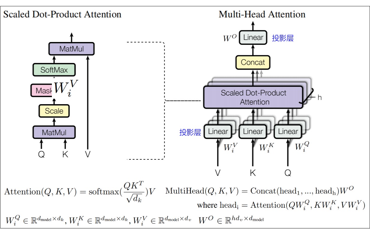
The original A12 architecture figure shows the paper equation and the wrapper around repeated scaled-dot-product attention calls:
Direct-sum output and the role of W_O
Let every head output have width d_v:
Concatenation places the head spaces side by side:
Partition W_O by its input rows:
Then the final output is:
This equation is more informative than “concatenate and project.” It shows
that each head writes through its own block of the output projection into the
shared residual width. W_O can rotate, amplify, suppress, and combine head
channels. It cannot, in general, reproduce a different pre-softmax routing
distribution because that would require moving a linear map across softmax.
The A12 calculation diagram follows the same sequence for several heads:
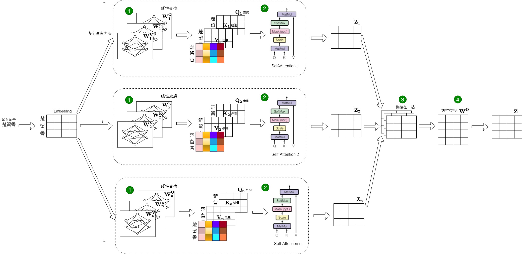
The figure’s Chinese token labels are only an example. The reusable semantic
path is numbered: project, compute each head, concatenate, then apply W_O.
Bias choices are part of the checkpoint contract
The four projections may include biases:
b_Q: [H*d_k]
b_K: [H*d_k]
b_V: [H*d_v]
b_O: [d_model]
With equal widths H*d_k = H*d_v = d_model, enabling all four adds
4*d_model parameters on top of 4*d_model^2. This is small in count but not
semantically ignorable. A bias-free LLaMA-style checkpoint cannot load into a
bias-enabled module by silently inventing values unless the conversion policy
sets and records them explicitly.
Bias also changes which rows can be zero. Even if an input state is zero, a
projection bias can produce nonzero Q/K/V. That can matter for PAD rows,
zero-initialized adapter paths, and tests that assume linear(0)=0.
The correct implementation question is not “does attention require bias?” It is:
which checkpoint architecture was trained;
which tensors are present in its state dictionary;
which projection orientation and packing the runtime expects;
whether a conversion preserves the same affine maps.
Head count changes width allocation, not only parallelism
At fixed d_model, choosing H determines d_head=d_model/H. This creates a
representation tradeoff:
more heads:
    more independently normalized routing matrices
    fewer feature channels in each Q/K/V interaction

fewer heads:
    fewer routing matrices
    wider per-head comparison and value spaces
The score tensor contains B*H*Q*K elements even though the leading score
matmul MAC count simplifies to B*Q*K*d_model. More heads can therefore change
softmax reductions, launch geometry, temporary state, and numerical behavior
without changing the simplified arithmetic expression. Hardware divisibility
constraints can also make one head count substantially faster than another.
There is no architecture-only optimum. The original Transformer ablation, modern scaling studies, checkpoint compatibility, and target kernels all refer to particular width/depth/workload regimes.
Equal-width heads are an implementation design, not a mathematical law
Classic packed MHA chooses one width:
That gives one rectangular projection, one view, and one batched attention
kernel. Attention itself does not require every head to have the same Q/K or
value width. A heterogeneous design could use:
with per-head maps:
and scale head i by sqrt(d_i^k). Concatenation then produces width
d_concat, followed by:
The potential benefit is non-uniform capacity allocation: heads that need a wider matching or value space can receive it while others remain narrow. The systems cost is loss of the simple packed representation:
one view cannot describe ragged head widths;
heads may require separate or width-grouped projections;
score kernels see different D dimensions;
checkpoint slicing needs an explicit offset table;
tensor parallel partitioning becomes less regular;
pruning or growing one head changes W_O input layout.
This design axis is related to, but distinct from, head pruning. Pruning sets a head’s effective width to zero after or during training. Heterogeneous heads allocate different nonzero widths as part of the architecture. It is also distinct from MOHSA, which overlaps channels between heads, and from GQA, which changes the number of K/V heads shared by query heads.
Equal width remains the reference because it matches the canonical Transformer
and common checkpoints. The broader lesson is that H alone does not specify
head capacity. A comparison must report total projection width, every Q/K/V
head width, and the output projection layout.
Capacity for specialization is not proof of unique head roles
Different projection parameters make distinct behavior possible, but training does not guarantee that every head learns a unique, human-readable function. Michel et al. found that many trained heads in several Transformer models could be removed at test time with little performance loss. Some heads matter; others can be redundant or compensate for one another.
Use the narrow claim:
safe:
    multiple learned projection sets permit multiple routing distributions

too strong:
    every head necessarily learns one distinct linguistic relation

also wrong:
    heads are only a reshape with no parameterization consequence
This distinction is useful when reading attention maps. A visible pattern can be evidence about one trained head, but the architecture alone does not assign that head a semantic label.
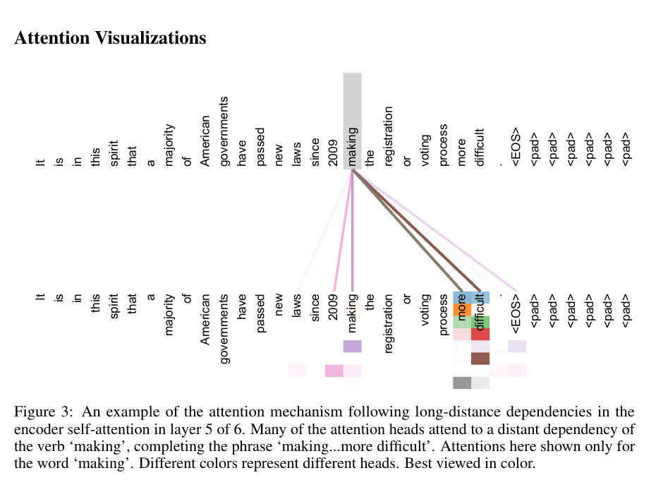
Source: Attention Is All You Need, Figure 3. The colored connections are empirical attention weights for the word making in encoder layer 5 of 6, not predefined head roles. The figure supports the narrow claim that trained heads can realize different routing patterns; it does not prove that every head is unique, linguistic, or causally necessary.
Head identity is not fixed under permutation
Before interpreting head number 3 as a stable concept, notice a symmetry in
the parameterization. If we permute the Q/K/V head slices and apply the inverse
permutation to the corresponding input blocks of W_O, the module computes the
same function. Head index is therefore a storage coordinate, not an inherent
semantic identity.
Let Pi be a permutation of head blocks. Then, schematically:
Training breaks symmetry through initialization and data, so individual heads can specialize. The architecture does not predetermine which index acquires which behavior, and different training runs can allocate related functions to different heads.
Visualization, ablation, and causal importance answer different questions
An attention heatmap shows the routing weights produced for selected examples. It does not by itself show how much a head changes model output because:
the value vectors may carry little or large downstream signal;
W_O can amplify, suppress, or combine the head output;
other heads and later layers can compensate;
an attractive pattern can correlate with, rather than cause, a prediction.
Michel et al. and Voita et al. used head masking/pruning experiments and found substantial redundancy in their evaluated models, while also identifying heads whose removal mattered more. Those are source-reported empirical results, not a proof that a fixed fraction of heads can be removed from every checkpoint.
A useful evidence ladder is:
| Evidence | Supports | Does not establish alone |
|---|---|---|
| attention map | a routing pattern occurred | causal necessity |
| gradient/sensitivity | local output dependence | robustness to retraining or removal |
| ablation | effect of removing/masking a head in a checkpoint | same effect after fine-tuning or kernel changes |
| prune + retrain | recoverability under a training procedure | universal redundancy ratio |
What trained head patterns can and cannot establish
A12 retained examples from BERT analysis in which some heads attended broadly, some followed nearby positions, and some concentrated on separator or punctuation tokens:
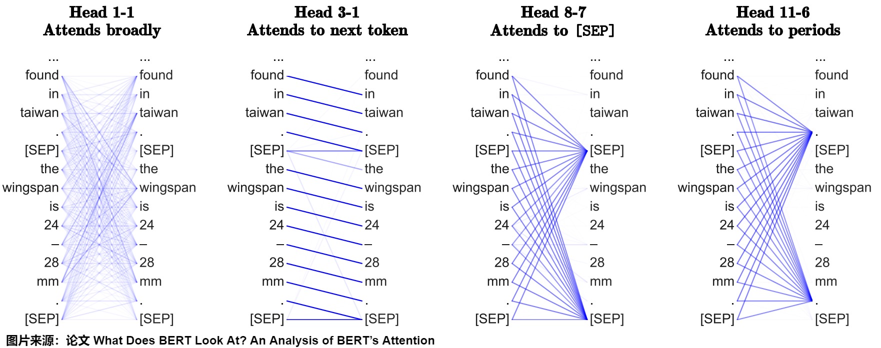
These patterns are useful observations about a trained checkpoint. They do not mean the architecture assigned four named jobs before training. Several causes can produce a visible pattern:
Q/K projections make one relation easy to score;
position information biases nearby or fixed-offset matches;
special-token states become convenient global aggregation points;
the value path and W_O make only part of the visible routing useful;
later layers compensate for or reinterpret earlier routing.
Head behavior can also vary by layer. Lower layers may show more local or surface patterns in one model while upper layers show broader task-conditioned patterns, but that is an empirical trend, not a fixed hierarchy law. Model family, objective, tokenization, architecture, and random seed can all change the allocation.
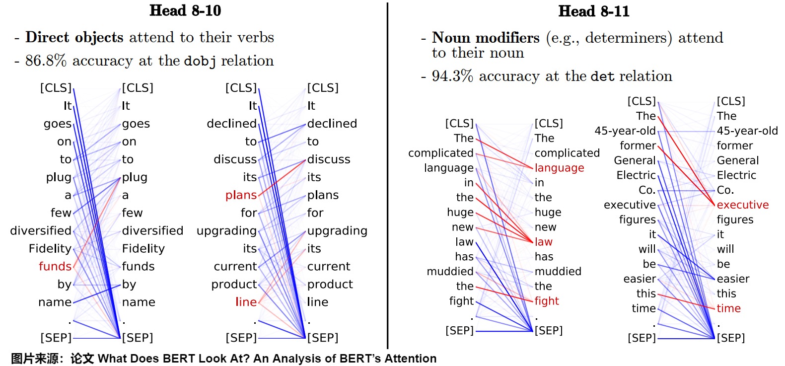
Source: Clark et al., What Does BERT Look At?, with A12’s retained footer. These are examples from particular BERT heads and dependency relations. The reported accuracies do not establish that the same numbered heads, relations, or causal importance recur across checkpoints.
Head gates, pruning objectives, and retraining
To test whether a head is needed, insert scalar gate g_i on its output:
Setting one g_i=0 performs an ablation. Learning sparse gates adds a penalty,
schematically:
The indicator is non-differentiable, so practical methods use continuous relaxations, importance scores, stochastic gates, or iterative prune/retrain procedures. A12 preserved the source idea that specialized heads can do much of the work while others are removable:
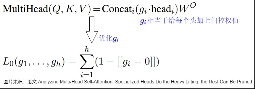
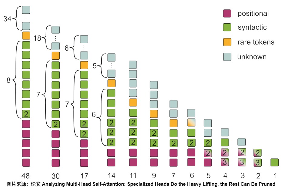
Source: Voita et al., Analyzing Multi-Head Self-Attention, with A12’s retained footer. The columns record one paper’s learned-gate/pruning outcome; they are not a universal pruning schedule or a fixed taxonomy assigned by the architecture.
Three results must be kept separate:
zero-shot ablation:
    remove a head without updating any other parameter

fine-tuned pruning:
    allow remaining heads and W_O to compensate

architecture retraining:
    train a smaller-head model from the beginning
They answer different questions. A checkpoint may tolerate zeroing many heads because its representation is redundant, while a smaller architecture trained from scratch follows a different optimization path.
Head dropout is not attention-probability dropout
Attention dropout removes individual query-key probability links. Head dropout
removes an entire O_i branch for selected tokens or batches. With inverted
scaling, a head-level mask can regularize dependence on one head:
head_mask = bernoulli_keep([B, H, 1, 1]) / keep_probability
head_outputs = head_outputs * head_mask
This changes gradient coupling through W_O and can encourage redundancy, but
it also changes the training/runtime mismatch if every head is active at
inference. It should be documented separately from:
attention dropout: edges within each head
head pruning: permanent architecture/checkpoint change
MoH routing: input-dependent selected head set
GQA/MQA: shared K/V parameter and cache structure
Specialization needs a complete evidence tuple
A serious head claim should report at least:
checkpoint and layer/head index;
input examples and tokenization;
whether weights are pre- or post-dropout;
the attention pattern;
the value/output contribution or ablation effect;
whether the model was fine-tuned after intervention.
Without that tuple, “this head detects syntax” is an interpretation. It may be useful for forming a hypothesis, but it is not yet a causal mechanism claim.
How a head trains through concat and W_O
Write each per-head output as O_h: [B,Q,D] and concatenate:
The module output is:
During backward, incoming gradient G_Y first reaches the concatenated space:
Slicing G_cat by head gives the gradient sent to each O_h. This means
W_O participates in deciding which combinations of head channels help the
loss. A head is not trained against an independent objective; all heads are
coupled through the shared downstream loss and output projection.
The per-head gradient then follows M3.1 through P_hV_h, softmax, scores, and
Q/K/V projections. This coupling explains two observations that are otherwise
easy to treat as contradictory: heads can learn visibly different routing
patterns, and yet another head or W_O can sometimes compensate when one head
is removed.
0x03 Inputs: self-attention and cross-attention use the same module
The forward signature is:
def forward(self, query, key, value, mask=None):
The names here are not yet the per-head Q/K/V tensors consumed by M3.1. They are input state rows that will be projected inside this module.
For encoder self-attention:
self.self_attn(x, x, x, src_mask)
Shape:
query/key/value input: [B,S,d_model]
For decoder causal self-attention:
self.self_attn(x, x, x, tgt_mask)
Shape:
query/key/value input: [B,T,d_model]
For decoder cross-attention:
self.src_attn(x, memory, memory, src_mask)
Shape:
query input: [B,T,d_model]
key input:   [B,S,d_model]
value input: [B,S,d_model]
So the module does not require q_len == k_len. It only requires that the row width of each input is d_model, and that key/value sequence lengths agree for the later attention call.
Cross-attention is a target-indexed read from source memory
The shared module signature can hide the most important encoder-decoder invariant. In a decoder layer, the calls are ordered:
def forward(self, x, memory, src_mask, tgt_mask):
    x = self.sublayer[0](x, lambda x: self.self_attn(x, x, x, tgt_mask))
    x = self.sublayer[1](x, lambda x: self.src_attn(x, memory, memory, src_mask))
    return self.sublayer[2](x, self.feed_forward)
The target self-attention call first updates each target row from its legal target history. That updated target state becomes the cross-attention query. The encoder output is persistent source memory and supplies keys and values:
Q_cross <- target state after causal self-attention
K_cross <- encoder memory
V_cross <- encoder memory
After projection and head splitting:
Q_cross: [B,h,T,d_head]
K_cross: [B,h,S,d_head]
V_cross: [B,h,S,d_value]
The score tensor follows directly:
Rows are target query positions. Columns are source memory positions. Softmax normalizes the source axis for every target row:
The value mix is:
The output length is T, because queries own output rows. Source information
has been mixed into target-indexed state; cross-attention does not replace the
target stream with an encoder-length stream.
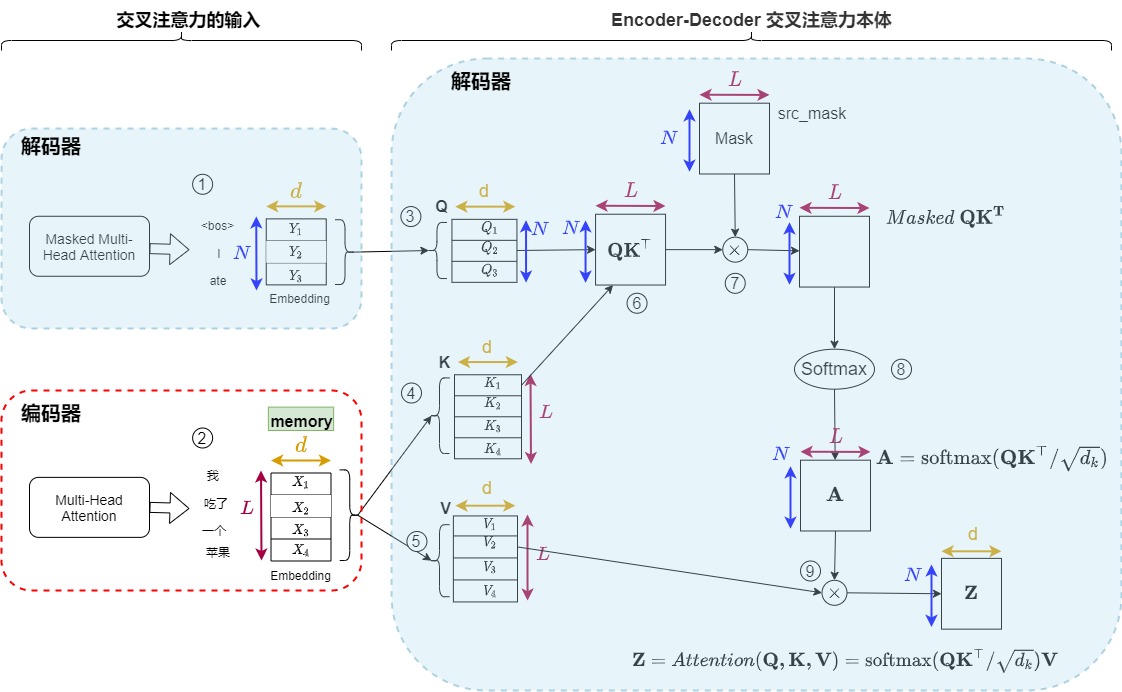
The source visual labels target length as N and source length as L. In this
article those axes are T and S; the invariant is the same: the attention
matrix is target-by-source.
One target-by-source trace
Use source memory rows for:
I | ate | an | apple
and target-prefix rows:
<bos> | J' | ai | mange | une | pomme
For one head, a pedagogical cross-attention matrix could be:
                  source memory columns
                  I       ate      an      apple
target <bos>   [ 0.10    0.20    0.10    0.60 ]
target J'      [ 0.70    0.10    0.10    0.10 ]
target ai      [ 0.20    0.65    0.05    0.10 ]
target mange   [ 0.15    0.70    0.05    0.10 ]
target une     [ 0.05    0.10    0.55    0.30 ]
target pomme   [ 0.05    0.05    0.10    0.80 ]
This is not a claim that trained attention heads are clean word aligners.
Weights may be diffuse, syntactic, position-biased, redundant, or difficult to
interpret. The table exists to make the axes auditable. The row for pomme
mixes source value rows and writes the result back into the target row for
pomme.
Two shape-correct errors follow from this trace:
softmax over T instead of S:
    source columns distribute mass across target rows
    rather than each target row reading source memory

target causal mask used as src_mask when T == S:
    shape may broadcast
    but source columns are incorrectly treated as future target positions
Source-memory lifetime and projected K/V reuse
The encoder usually runs once for a supplied source and returns:
memory: [B,S,d_model]
Every decoder layer reads that memory, but each layer has its own cross-attn
W_K and W_V. During autoregressive inference, an implementation can project
source memory once per layer and retain:
K_cross_cache[layer]: [B,h,S,d_head]
V_cross_cache[layer]: [B,h,S,d_value]
Those tensors are different from target self-attention K/V cache:
| State | Sequence axis | Growth during decode | Source |
|---|---|---|---|
| encoder memory | S | fixed | encoder output |
| projected cross K/V | S | fixed | per-layer projections of encoder memory |
| target self-attention K/V | decoded prefix length | grows one accepted token at a time | decoder target states |
The optimization choice is a memory/compute trade. Reprojecting encoder memory spends repeated GEMMs; retaining projected K/V spends layer-specific memory. M5 owns the serving policy, but M3.2 must identify the reusable tensors and their owners.
For classic MHA, one layer retains 2BSd_model K/V elements. With B=4,
S=512, d_model=768, and two bytes per element:
2 * 4 * 512 * 768 * 2 bytes = 6 MiB per decoder layer
Six decoder layers retain 36 MiB before allocator metadata or other runtime state. The number is not an argument to always cache or always recompute. It is the state ledger required to make the decision.
Training execution: one memory, many target rows, full backward paths
During teacher-forced encoder-decoder training, the encoder normally produces
memory once for the source batch. The decoder receives all shifted target
rows and each decoder layer performs:
target causal self-attention: [B,H,T,T]
cross-attention:              [B,H,T,S]
The original decoder structure makes the order visible:
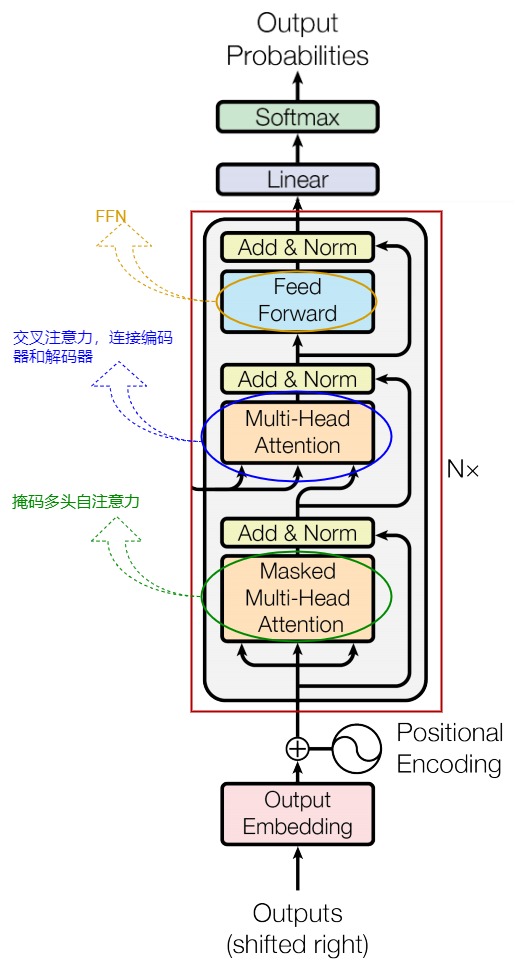
All target queries in a training batch can reuse the same projected source K/V within a layer. Whether the implementation computes those projections as part of one batched call or explicitly precomputes them does not change the mathematical graph.
Backward follows both streams:
loss
  -> decoder output and residual stack
    -> cross-attention W_O and head outputs
      -> Q branch -> target-side decoder state
      -> K/V branches -> encoder memory
        -> encoder layers and source embeddings
If the encoder is frozen, the runtime may detach memory deliberately. If it is
not frozen, an accidental .detach() or cache wrapper that drops autograd
history prevents cross-attention gradients from training the encoder. The
forward outputs still have valid shapes.
For one decoder layer, write:
The memory gradient is the sum of key and value paths:
Across L_dec decoder layers, memory receives one such contribution from each
layer, followed by the encoder-side backward graph. Reusing the same memory
object is therefore not the same as sharing cross-attention projection weights:
each decoder layer has its own W_K, W_V, and gradient contribution.
Autoregressive execution: static source state, growing target state
After encoding, source length S is fixed while target decode length grows.
At decode step t, one common shape contract is:
target query:       [B,H,1,D]
cross K/V:          [B,H,S,D]       fixed for the request
self-attention K/V: [B,H,t,D]       grows with accepted target tokens
The A12 source retained a full MHA execution diagram with cached K/V rows. It mixes residual/norm and kernel detail, but its useful runtime distinction is the current query against previously retained key/value state:
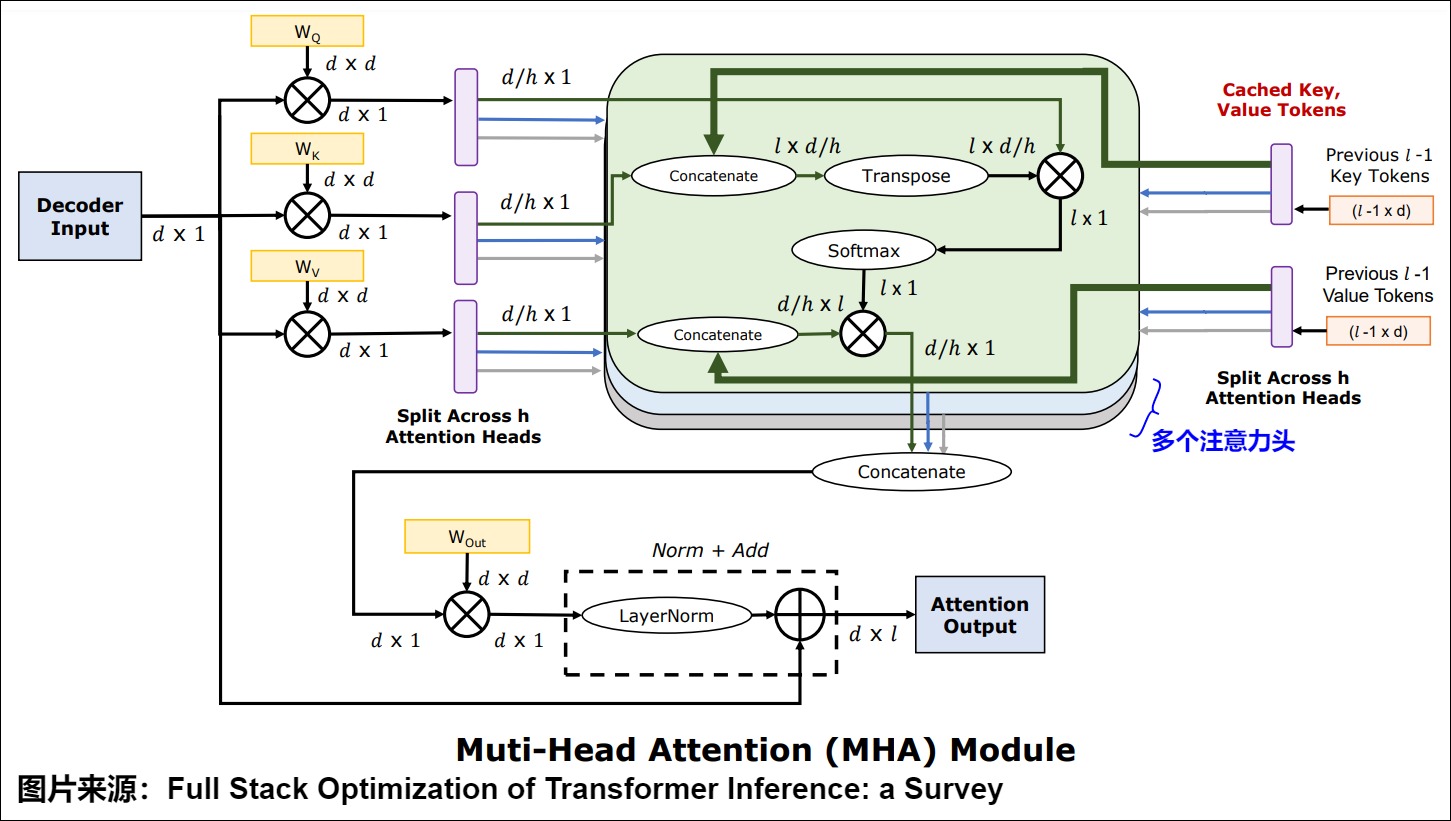
For cross-attention, source K/V are not appended each target step. They can be created once per decoder layer:
class CrossAttentionState:
    def __init__(self, memory, layers):
        self.memory = memory
        self.projected = []
        for layer in layers:
            k = split_heads(layer.cross_attn.k_proj(memory))
            v = split_heads(layer.cross_attn.v_proj(memory))
            self.projected.append((k, v))

def decode_cross_step(layer, target_row, cross_state, layer_id, src_visible):
    q = split_heads(layer.cross_attn.q_proj(target_row))
    k, v = cross_state.projected[layer_id]
    o = scaled_dot_product_attention(q, k, v, visible=src_visible)
    return layer.cross_attn.o_proj(merge_heads(o))
This sketch assumes parameters are fixed during generation and the source memory does not change. It is invalid across a weight update, adapter switch, encoder-memory mutation, or source edit unless the projected state is rebuilt.
The alternative is recomputation:
k = split_heads(k_proj(memory))
v = split_heads(v_proj(memory))
at every target step. That saves persistent cross-KV state but repeats projection work. The crossover depends on source length, number of decode steps, layer count, memory capacity, projection/kernel efficiency, and whether the workload batches many targets for the same source.
Beam search changes ownership, not source content
With beam width G, several hypotheses share one encoded source. A naïve
implementation expands memory and projected cross K/V:
memory: [B,S,D] -> [B*G,S,D]
cross K/V: [B,H,S,Dh] -> [B*G,H,S,Dh]
Physical replication can multiply memory by G. A runtime can instead keep
one source state per request and maintain a beam-to-source index:
source_id = beam_source_index[beam_id]
k = cross_k[layer][source_id]
v = cross_v[layer][source_id]
Target self-attention caches still diverge by hypothesis because each beam has a different generated prefix. Cross K/V remain source-owned. Beam reordering must therefore reorder target caches and beam metadata without corrupting the source mapping.
This distinction is easy to miss when code calls repeat_interleave on every
tensor for convenience. Logical broadcasting, indexed sharing, and physical
replication produce the same values but different memory behavior.
Cross-attention state invalidation
Projected source K/V are derived state. A serving or evaluation system needs a cache key containing every object that can change them:
model/checkpoint identity;
decoder layer identity;
active adapter or fine-tuning state;
source tokenization and encoder output;
position/geometry policy applied to source K/V;
dtype, device, tensor-parallel shard, and projection layout.
Reusing cross K/V after changing one of these objects can be shape-correct and numerically wrong. This is analogous to target KV-cache invalidation, but the state is fixed-length and source-conditioned.
Full call graph and ownership boundary
A4 preserved a code-level graph from batch masks through encoder, decoder, the two attention call sites, and the local attention function:
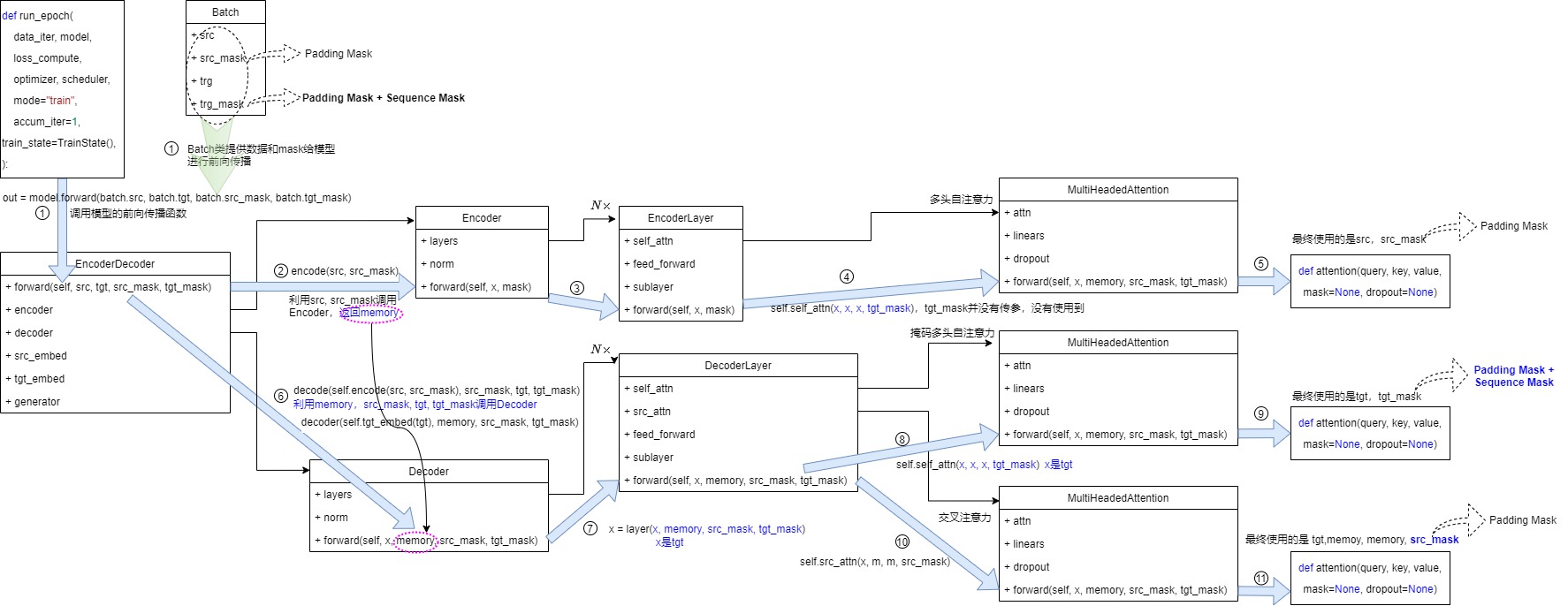
Read the dense source figure through four invariants:
encoder self-attention:
    Q/K/V all come from source-indexed state

decoder self-attention:
    Q/K/V all come from target-indexed state and use target visibility

decoder cross-attention:
    Q comes from target state; K/V come from encoder memory

local attention:
    the same M3.1 score path executes after projection/head layout
M3.2 owns these module inputs, projected layouts, and reusable source state. M3.10 will own the complete request loop, and M5 owns multi-request scheduling and memory policy.
Cross-attention integration assertions
def cross_attention_inputs(target_state, memory, src_visible):
    B, T, d = target_state.shape
    Bm, S, dm = memory.shape
    assert B == Bm and d == dm
    assert src_visible.shape[-1] == S

    q = target_state
    k = memory
    v = memory
    return q, k, v
After the module call:
cross_out = src_attn(target_state, memory, memory, src_visible)
assert cross_out.shape == target_state.shape
That final assertion is more than a convenience. It states that residual addition is target-indexed and that source length must not leak into the output sequence axis.
0x04 Mask head-axis insertion
The first line in forward is:
if mask is not None:
    mask = mask.unsqueeze(1)
A12 explains the reason: after head splitting, the score tensor has a head axis.
For a target mask:
before: [B, T, T]
after:  [B, 1, T, T]
Then it can broadcast over heads:
scores: [B, h, T, T]
mask:   [B, 1, T, T]
For source padding:
before: [B, 1, S]
after:  [B, 1, 1, S]
scores: [B, h, q_len, S]
M3.2 only owns the head-axis insertion. M3.1 owns how the mask is applied to scores. M3.9 owns training-mask construction.
0x05 Head-packed Q/K/V projection
The projection path is:
query, key, value = [
    lin(x).view(nbatches, -1, self.h, self.d_k).transpose(1, 2)
    for lin, x in zip(self.linears, (query, key, value))
]
The zip pairs the first three linears with the three inputs:
W_Q applied to query input
W_K applied to key input
W_V applied to value input
For self-attention, all three inputs are the same x, but the projections are still different learned matrices:
Q = W_Q x
K = W_K x
V = W_V x
For cross-attention:
Q = W_Q decoder_state
K = W_K encoder_memory
V = W_V encoder_memory
The first step preserves model width:
lin(query_input): [B,q_len,d_model] -> [B,q_len,d_model]
lin(key_input):   [B,k_len,d_model] -> [B,k_len,d_model]
lin(value_input): [B,k_len,d_model] -> [B,k_len,d_model]
That output is then reinterpreted as heads:
[B,*,d_model] -> [B,*,h,d_k]
This is a layout operation after projection, not a new attention computation and not a pre-projection chunking of the original row.
The wording matters: the Harvard module has three separate projection
modules, and each projection packs all of its heads into one d_model-wide
output. This is different from a modern fused QKV projection that packs Q,
K, and V into one larger matrix multiplication.
Parameter orientation: equation versus framework storage
Mathematical prose often writes row-major activations as:
PyTorch nn.Linear(in_features, out_features) stores weight as:
weight: [out_features, in_features]
and evaluates the equivalent operation:
q = F.linear(x, weight_q, bias_q) # x @ weight_q.T + bias_q
For classic equal-width MHA:
equation W_Q:       [d_model,d_model]
PyTorch weight_q:   [d_model,d_model]
The dimensions happen to be square, so a mistaken transpose is invisible in a shape ledger. The values are still wrong. This becomes easier to detect for GQA/MQA or asymmetric projections where output width differs from input width.
Separate projections
The Harvard path is structurally:
q = q_proj(query_input)  # [B,Q,d_model]
k = k_proj(key_input)    # [B,K,d_model]
v = v_proj(value_input)  # [B,K,d_model]
Separate modules are natural for cross-attention because query and memory lengths differ and can come from different calls. They also make parameter names explicit in checkpoints.
One fused QKV projection
Decoder-only self-attention often uses one projection whose output contains all three tensors:
qkv = qkv_proj(x)                    # [B,S,3*d_model]
q, k, v = qkv.split(d_model, dim=-1)
Ignoring bias, the equation is:
In PyTorch storage, concatenation is usually over the output-row axis:
weight_qkv = torch.cat([weight_q, weight_k, weight_v], dim=0)
# [3*d_model, d_model]
One larger GEMM can reduce launch and input-read overhead. It does not tie Q/K/V weights; they still occupy separate slices. It also does not directly apply to cross-attention when Q and K/V come from different input tensors. A common cross-attention layout uses one Q projection and one fused KV projection:
q = q_proj(target_state)             # [B,T,d_model]
kv = kv_proj(source_memory)          # [B,S,2*d_model]
k, v = kv.chunk(2, dim=-1)
Checkpoint conversion is a storage transform, not a model rewrite
def fuse_qkv(q_proj, k_proj, v_proj):
    fused_weight = torch.cat(
        [q_proj.weight, k_proj.weight, v_proj.weight], dim=0
    )
    fused_bias = None
    if q_proj.bias is not None:
        fused_bias = torch.cat([q_proj.bias, k_proj.bias, v_proj.bias], dim=0)
    return fused_weight, fused_bias

def split_qkv(fused_weight, fused_bias=None):
    q_w, k_w, v_w = fused_weight.chunk(3, dim=0)
    if fused_bias is None:
        return (q_w, None), (k_w, None), (v_w, None)
    q_b, k_b, v_b = fused_bias.chunk(3, dim=0)
    return (q_w, q_b), (k_w, k_b), (v_w, v_b)
Real checkpoints can use interleaved head order, grouped K/V widths, tensor parallel shards, quantized packed formats, or fused bias conventions. A correct converter must verify ordering with an output-parity test, not only compare parameter counts.
0x05A Per-head maps, packed storage, and complete accounting
The compact identity [Q K V] = X[W_Q W_K W_V] is sufficient only for
self-attention with one input stream. To reconcile per-head equations,
rectangular cross-attention, asymmetric value width, framework storage, and a
checkpoint byte ledger, keep the three source tensors explicit:
For head i, define right-multiplication maps and biases:
The explicit head tensors are:
Each map may read all D_m input channels. The per-head width constrains the
output of the map; it does not partition the residual row before learning.
Why horizontal concatenation gives the packed projection
Concatenate the logical maps along their output columns:
and concatenate the biases in the same head order:
Matrix multiplication distributes over a block-column matrix:
Therefore reshaping [B,Q,H*D_qk] into [B,Q,H,D_qk] exposes exactly the
explicit head results. It does not approximate or tie them. The same proof
holds for K and V, with K using source length K and V using width D_v.
The equality depends on one ordered convention. If the packed columns are
[head_1,head_0,...] while the checkpoint manifest says
[head_0,head_1,...], shapes and parameter counts remain valid but head values
do not reconcile.
Framework storage is the transpose of the logical map
For a framework linear operation:
y = x @ weight_stored.T + bias
the stored packed Q tensor is:
Fusing Q, K, and V concatenates these stored rows:
One input can use that fused map in self-attention. Cross-attention still needs
at least a target Q multiplication and a source KV multiplication because
X_q and X_kv are different objects. A fused checkpoint can remain useful as
a persistence format, but execution must split or gather the correct spans
before applying them to different streams.
The conversion proof has three independent gates:
byte gate:
    split(fuse(W_Q,W_K,W_V)) reproduces every stored tensor and bias exactly

projection gate:
    explicit per-head == packed-separate == packed-fused slices

call gate:
    each role is applied to the state id declared in the immutable manifest
Passing only the byte gate does not prove that Q and K were applied to the right streams. Passing only output shape does not prove either gate.
Parameter count from map dimensions
With Q and K width HD_qk, V/merged width HD_v, and all four biases enabled:
Thus:
Without biases, remove the final four terms. In canonical equal-width MHA,
D_qk=D_v=D_m/H, so:
The apparent head-count cancellation is conditional on shrinking each head as
1/H. Holding D_qk and D_v fixed while increasing H increases projection
width and parameter count linearly.
Forward MAC ledger from contracted dimensions
Count one multiply-accumulate as one MAC. The projection and output terms are:
The two head-local products consumed from M3.1 contribute:
Therefore:
This is a logical arithmetic ledger, not a latency model. It excludes softmax, mask conversion, dropout, bias additions, reads/writes, launch overhead, and backend-dependent fusion. M4 owns measured kernel and traffic analysis.
Checkpoint bytes and activation elements are different ledgers
For uniform parameter storage of b_p bytes per scalar:
Fusion does not change this value when it only concatenates the same Q/K/V/O weights and biases. Quantization, padding, scales, metadata, and tensor-parallel shards can change persistent bytes and must be counted separately.
The principal projected activation element counts before score materialization are:
Q packed: B * Q * H * D_qk
K packed: B * K * H * D_qk
V packed: B * K * H * D_v
merged:   B * Q * H * D_v
output:   B * Q * D_m
They are not parameters and should not be multiplied by checkpoint dtype. A runtime may save, recompute, cast, or fuse them under a separate liveness contract.
Numeric rectangular reconciliation
Use the immutable asymmetric fixture:
B=2, Q=3, K=4, D_m=6, H=2, D_qk=3, D_v=2
The Q/K packed widths are 6, the V/merged width is 4, and fused QKV storage has 16 rows. With all biases enabled:
| Object | Weights | Bias | Parameters |
|---|---|---|---|
| Q | 6*6=36 | 6 | 42 |
| K | 6*6=36 | 6 | 42 |
| V | 6*4=24 | 4 | 28 |
| O | 4*6=24 | 6 | 30 |
| total | 120 | 22 | 142 |
At four bytes per parameter, the unpadded FP32 checkpoint payload is 568 bytes. The forward MAC ledger is:
| Term | Calculation | MACs |
|---|---|---|
| Q projection | 2*3*6*6 | 216 |
| K projection | 2*4*6*6 | 288 |
| V projection | 2*4*6*4 | 192 |
| score product | 2*2*3*4*3 | 144 |
| probability-value product | 2*2*3*4*2 | 96 |
| output projection | 2*3*4*6 | 144 |
| total | 1,080 |
The executable oracle constructs deterministic per-head maps, packs them, transposes them into framework storage, fuses/splits the checkpoint, and checks elementwise equality. It also executes the plausible alternative “split the raw residual row into heads, then project locally.” That alternative is a block-diagonal architecture with fewer cross-channel connections; it does not reproduce canonical MHA merely because its final head shape matches.
0x06 Head split: view(...).transpose(1, 2)
The split line has two important operations:
lin(x).view(nbatches, -1, self.h, self.d_k).transpose(1, 2)
First, view splits the last dimension:
projected query: [B,q_len,d_model]
view query:      [B,q_len,h,d_k]

projected key:   [B,k_len,d_model]
view key:        [B,k_len,h,d_k]
Then transpose(1, 2) moves the head axis before the sequence axis:
query view:       [B,q_len,h,d_k]
query transpose:  [B,h,q_len,d_k]

key view:         [B,k_len,h,d_k]
key transpose:    [B,h,k_len,d_k]
This layout matches M3.1’s attention function:
query: [B,h,q_len,d_k]
key:   [B,h,k_len,d_k]
value: [B,h,k_len,d_k]
For cross-attention, the -1 sequence dimension is inferred separately for each input:
query input length T -> query: [B,h,T,d_k]
key input length S   -> key:   [B,h,S,d_k]
value input length S -> value: [B,h,S,d_k]
That is why the same code can handle self-attention and cross-attention.
0x07 Batched attention over heads
After projection and transpose, the call is:
x, self.attn = attention(
    query, key, value, mask=mask, dropout=self.dropout
)
This is the M3.1 primitive, applied with the head axis present.
For encoder self-attention:
query:    [B,h,S,d_k]
key:      [B,h,S,d_k]
value:    [B,h,S,d_k]
scores:   [B,h,S,S]
out/head: [B,h,S,d_k]
For cross-attention:
query:    [B,h,T,d_k]
key:      [B,h,S,d_k]
value:    [B,h,S,d_k]
scores:   [B,h,T,S]
out/head: [B,h,T,d_k]
self.attn stores the attention probability tensor returned by M3.1:
self.attn: [B,h,q_len,k_len]
This is useful for inspection, but it is not the residual-stream output. The output that continues through the module is x, the weighted value result per head.
0x08 Concatenation: transpose, contiguous, view
After attention, x has one output vector per head:
x: [B,h,q_len,d_k]
The next lines merge the heads:
x = (
    x.transpose(1, 2)
    .contiguous()
    .view(nbatches, -1, self.h * self.d_k)
)
First, transpose the head and sequence axes:
[B,h,q_len,d_k] -> [B,q_len,h,d_k]
Then contiguous() makes the transposed tensor’s memory layout compatible with view. A12 calls this out explicitly. Without it, .view(...) fails with an error whenever the transposed strides cannot be folded into one h*d_k axis (with h > 1 and d_k > 1, that is any q_len > 1); it never silently reorders values. In newer PyTorch code, .reshape(...) often hides this detail, but checkpoint/debugging work still benefits from knowing why contiguous() is there.
Finally, fold the head and head-width axes:
[B,q_len,h,d_k] -> [B,q_len,h*d_k]
Because h * d_k = d_model, the merged object is:
x: [B,q_len,d_model]
That is the concatenation step in the original multi-head attention formula:
Why transpose changes strides even when shape math is valid
Assume the projected tensor [B,Q,H,D] is contiguous. Its logical strides are:
[Q*H*D, H*D, D, 1]
After transpose(1, 2), shape is [B,H,Q,D], but the underlying storage has
strides:
[Q*H*D, D, H*D, 1]
The head and query axes are views over interleaved storage. Transposing back to
[B,Q,H,D] restores the logical axis order, but relying on a later view to
merge H*D requires those dimensions to be contiguous in the expected order.
That is why the explicit sequence is:
merged = head_out.transpose(1, 2).contiguous().view(B, Q, H * D)
reshape may return a view when possible or allocate a contiguous copy when
necessary:
merged = head_out.transpose(1, 2).reshape(B, Q, H * D)
The second form is convenient, but it can hide the copy. In a profiling or kernel-fusion discussion, that hidden materialization is part of the runtime contract.
A stride-level test catches axis-preserving mistakes
B, Q, H, D = 2, 3, 4, 5
packed = torch.arange(B * Q * H * D).view(B, Q, H, D)
heads = packed.transpose(1, 2)

assert heads.shape == (B, H, Q, D)
assert not heads.is_contiguous()

round_trip = heads.transpose(1, 2).contiguous().view(B, Q, H * D)
expected = packed.view(B, Q, H * D)
torch.testing.assert_close(round_trip, expected)
A wrong transpose can preserve element count and final shape. Filling the tensor with distinct increasing values verifies that channel/head identity also survives the round trip.
0x08A Layout proof: shape, stride, storage, and row identity
Shape describes which logical coordinates exist. Stride describes how moving one unit along an axis changes the storage offset. A split/merge contract needs both.
For contiguous [B,S,H,D], the row-major element strides are:
The element at (b,s,h,d) occupies offset:
Flattening the last two axes defines channel index c=hD+d, so the packed
[B,S,HD] row has exactly the same offset:
This is why splitting a contiguous packed output axis is a legal view. The head and within-head coordinates are adjacent subdivisions of one packed channel axis.
Transpose changes axis interpretation, not storage bytes
After:
heads = packed.view(B, S, H, D).transpose(1, 2)
the logical shape is [B,H,S,D] and the element strides are:
Coordinate (b,h,s,d) still resolves to:
which is the same byte as original coordinate (b,s,h,d). No activation was
copied; only the axis-to-stride association changed. shares_storage=True and
is_contiguous=False are therefore both expected.
This distinction explains two failures that shape notation alone hides:
# Correct: split packed channel, then permute semantic axes.
correct = packed.view(B, S, H, D).transpose(1, 2)

# Wrong: relabel contiguous [B,S,H,D] bytes directly as [B,H,S,D].
wrong = packed.view(B, H, S, D)
Both objects have shape [B,H,S,D] when S and H use the declared extents.
The wrong version changes the coordinate-to-token mapping because its logical
iteration order assumes H was already before S in storage.
Why merge transposes back before flattening
The local attention output is logically [B,H,Q,D_v]. Head concatenation is
defined per query row:
The implementation therefore first returns to [B,Q,H,D_v]:
token_major = head_out.transpose(1, 2)
Its strides become compatible with the original token-major ordering. Calling
contiguous() materializes that order when needed, then view(B,Q,H*D_v)
folds adjacent H and D_v axes.
Directly executing:
wrong = head_out.reshape(B, Q, H * D_v)
does not mean “transpose and merge.” reshape preserves the logical iteration
order of [B,H,Q,D_v]; if it copies, it copies head-major rows. The result has
the requested [B,Q,H*D_v] shape but mixes which query positions occupy each
row. A convenience function cannot infer the semantic permutation you omitted.
view, reshape, and contiguous have different contracts
| Operation | Semantic effect | Storage effect | Failure mode |
|---|---|---|---|
view | changes extents while preserving one compatible stride mapping | shares storage | rejects incompatible noncontiguous folding |
transpose / permute | reorders logical axes | usually shares storage with new strides | later code may assume contiguity |
reshape | requests new extents, not an axis permutation | returns a view or allocates a copy | hides materialization; cannot repair omitted permutation |
contiguous | preserves logical values/order | returns contiguous storage, copying when required | adds traffic and temporary liveness |
as_strided | assigns arbitrary extents/strides | shares storage | overlap or wrong coordinates can remain shape-valid |
reshape is safe when the desired logical ordering has already been expressed.
It is not a substitute for naming the correct axes. contiguous() is not
mathematically part of MHA, but its possible copy is operationally observable
and must not disappear from a memory or latency ledger.
Rectangular and asymmetric paths need separate traces
The immutable asymmetric call produces:
Q packed [2,3,6] -> view [2,3,2,3] -> heads [2,2,3,3]
K packed [2,4,6] -> view [2,4,2,3] -> heads [2,2,4,3]
V packed [2,4,4] -> view [2,4,2,2] -> heads [2,2,4,2]
Using one cached (S,D) pair for all three roles would silently turn V’s
within-head width from 2 into 3 or force an impossible view. Inferring -1 for
the sequence axis is safe only when H and the role-specific width are already
frozen and the packed element count reconciles exactly.
After the local value mixture:
head output [2,2,3,2]
    -> transpose [2,3,2,2]
    -> contiguous/reshape [2,3,4]
The merged width is H*D_v=4, not Q/K width 6 and not automatically
D_model. W_O then maps [2,3,4] to [2,3,6].
Executable row-identity oracle
Random tensors can make a permutation error hard to localize. The layout oracle uses values whose digits encode the logical coordinates:
value(b,s,h,d) = 1000*b + 100*s + 10*h + d
It checks:
heads[b, h, s, d] == packed_bshd[b, s, h, d]
merged[b, s, h*D + d] == heads[b, h, s, d]
and records shape, element strides, contiguity, and storage sharing at every transition. Two invalid paths deliberately preserve final extents:
- direct
[B,S,H,D] -> [B,H,S,D]view without transpose; - direct
[B,H,S,D] -> [B,S,H*D]reshape without returning to token-major order.
Both differ from the reference, so a shape-only test would be insufficient. The oracle also verifies that Q, K, and V rectangular/asymmetric traces each round-trip independently.
0x09 Output projection W_O
The final line is:
return self.linears[-1](x)
This is the output projection:
W_O: [d_model,d_model]
It maps the concatenated head result back into the model’s residual-stream width:
x before W_O: [B,q_len,d_model]
x after W_O:  [B,q_len,d_model]
The shape stays the same, but the learned projection matters. Concatenating heads merely places their channels side by side. W_O mixes those channels into the representation that the next sublayer receives.
Omitting W_O is not a harmless simplification when reproducing a Transformer checkpoint. It changes the parameterization and the semantics of the residual update.
0x09A End-to-end reference module
The individual operations are easier to audit when assembled once. This reference deliberately supports unequal query and key lengths, keeps mask semantics explicit, and returns pre-dropout attention weights for tests. It is not a replacement for a fused production kernel.
class ReferenceMultiHeadAttention(nn.Module):
    def __init__(self, d_model, num_heads, dropout_p=0.0, bias=False):
        super().__init__()
        if d_model % num_heads != 0:
            raise ValueError("d_model must be divisible by num_heads")

        self.d_model = d_model
        self.num_heads = num_heads
        self.head_dim = d_model // num_heads
        self.dropout_p = dropout_p

        self.q_proj = nn.Linear(d_model, d_model, bias=bias)
        self.k_proj = nn.Linear(d_model, d_model, bias=bias)
        self.v_proj = nn.Linear(d_model, d_model, bias=bias)
        self.o_proj = nn.Linear(d_model, d_model, bias=bias)

    def split_heads(self, x):
        # x: [B,L,D_model]
        B, L, D = x.shape
        assert D == self.d_model
        x = x.view(B, L, self.num_heads, self.head_dim)
        return x.transpose(1, 2)  # [B,H,L,D_head]

    def merge_heads(self, x):
        # x: [B,H,Q,D_head]
        B, H, Q, Dh = x.shape
        assert H == self.num_heads and Dh == self.head_dim
        x = x.transpose(1, 2).contiguous()
        return x.view(B, Q, self.d_model)

    def forward(self, query_states, key_states, value_states, visible=None):
        B, Q, Dq = query_states.shape
        Bk, K, Dk = key_states.shape
        Bv, Kv, Dv = value_states.shape

        assert B == Bk == Bv
        assert Dq == Dk == Dv == self.d_model
        assert K == Kv

        q = self.split_heads(self.q_proj(query_states))
        k = self.split_heads(self.k_proj(key_states))
        v = self.split_heads(self.v_proj(value_states))

        scores = q @ k.transpose(-2, -1)
        scores = scores * (self.head_dim ** -0.5)
        assert scores.shape == (B, self.num_heads, Q, K)

        if visible is not None:
            visible = visible.to(device=scores.device, dtype=torch.bool)
            visible = torch.broadcast_to(visible, scores.shape)
            assert visible.any(dim=-1).all()
            scores = scores.masked_fill(~visible, -torch.inf)

        probabilities = torch.softmax(scores, dim=-1, dtype=torch.float32)
        probabilities = probabilities.to(q.dtype)
        dropped = torch.dropout(probabilities, self.dropout_p, self.training)

        head_output = dropped @ v
        merged = self.merge_heads(head_output)
        output = self.o_proj(merged)

        assert output.shape == (B, Q, self.d_model)
        return output, probabilities
The associated A12 implementation figure traces the same object sequence from
three projections through head views, per-head attention, merge, contiguity,
and W_O:
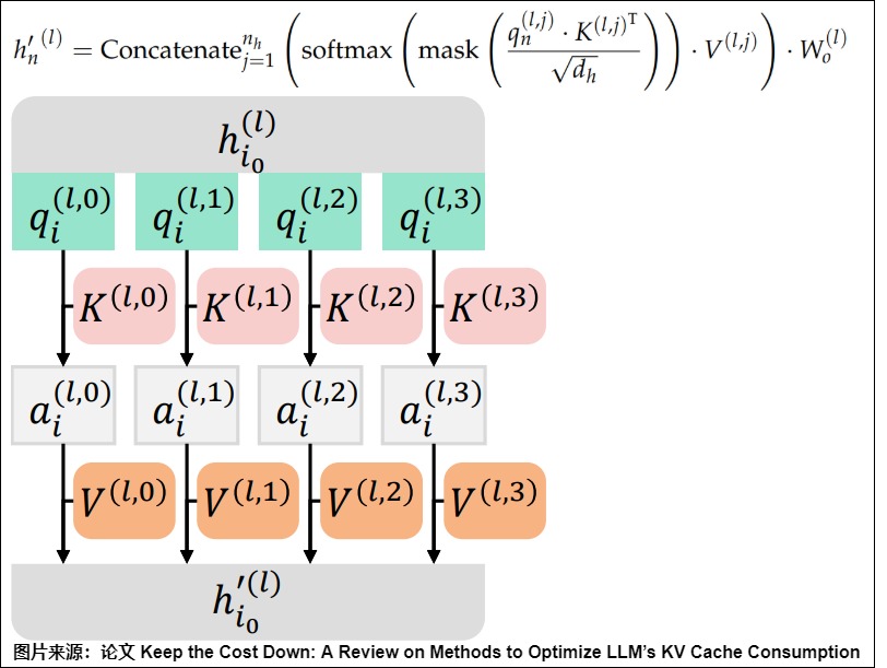
The figure uses seq_len for a self-attention example. The reference code
keeps Q and K separate so the same logic covers [B,H,T,S]
cross-attention.
Four execution traces through the same module
B, S, T, D, H = 2, 7, 5, 512, 8
mha = ReferenceMultiHeadAttention(D, H)

source = torch.randn(B, S, D)
target = torch.randn(B, T, D)

# Encoder self-attention: source rows read source rows.
enc_out, enc_p = mha(source, source, source)
assert enc_out.shape == (B, S, D)
assert enc_p.shape == (B, H, S, S)

# Decoder self-attention: target rows read legal target rows.
causal = torch.tril(torch.ones(T, T, dtype=torch.bool))[None, None]
dec_out, dec_p = mha(target, target, target, causal)
assert dec_out.shape == (B, T, D)
assert dec_p.shape == (B, H, T, T)

# Cross-attention: target rows read source rows.
source_real = torch.ones(B, 1, 1, S, dtype=torch.bool)
cross_out, cross_p = mha(target, source, source, source_real)
assert cross_out.shape == (B, T, D)
assert cross_p.shape == (B, H, T, S)

# One-row query against fixed source memory.
step_out, step_p = mha(target[:, -1:], source, source, source_real)
assert step_out.shape == (B, 1, D)
assert step_p.shape == (B, H, 1, S)
Using unequal S and T is deliberate. It prevents tests from accidentally
accepting a target mask on the source axis or reshaping cross K/V with query
length.
Packed projection versus explicit per-head equivalence
To verify a packed checkpoint conversion, slice the packed projection by head and compare:
packed = F.linear(x, packed_weight, packed_bias)  # [B,L,H*Dh]
packed = packed.view(B, L, H, Dh)

explicit = []
for head in range(H):
    lo = head * Dh
    hi = (head + 1) * Dh
    w_h = packed_weight[lo:hi, :]      # PyTorch [out,in]
    b_h = None if packed_bias is None else packed_bias[lo:hi]
    explicit.append(F.linear(x, w_h, b_h))

explicit = torch.stack(explicit, dim=2)  # [B,L,H,Dh]
torch.testing.assert_close(packed, explicit)
This catches transposed checkpoint slices, wrong concatenation order, and head-major/model-major layout assumptions.
Head-permutation equivalence test
Permuting Q/K/V head blocks must be paired with the inverse input-block
permutation of W_O. A conformance test can construct a random permutation,
transform all four matrices, and require identical output with dropout off.
permute Q head output blocks
permute K head output blocks with the same permutation
permute V head output blocks with the same permutation
permute W_O input columns to consume the new concat order
If only Q/K/V blocks are permuted, the per-head functions move but W_O
interprets their channels under the old order. If only W_O is permuted, the
same problem occurs in reverse.
Gradient gates for the assembled module
Forward equivalence is not enough for a conversion or custom kernel. Compare gradients for:
query, key, and value input states;
W_Q, W_K, W_V, and W_O;
optional projection biases;
cross-attention with Q != K length;
masked rows with at least one legal key;
training dropout under a controlled RNG state.
A backend can match output while sending a transposed or reduced gradient to one packed block. M3.1’s eager attention is the local score-path oracle; this module is the projection/layout oracle.
0x09B Output-block algebra, symmetry, and the wrapper adjoint
The preceding reference module establishes the forward object graph. A complete wrapper contract must also answer three harder questions:
which rows of W_O consume which head;
which simultaneous parameter transformations leave the function unchanged;
which gradients return to target state, source state, and every packed map.
These questions belong here because they are consequences of head packing and
caller ownership. M3.1 still owns the local attention derivative from one
head’s incoming dO_i to its dQ_i, dK_i, and dV_i.
W_O is a sum of head-specific residual-width writes
Let one batch/query row be understood and write each head result as
O_i in R^(d_v). Concatenation is a direct sum:
Partition the input rows of the logical output map:
Block multiplication then gives
This derivation matters for pruning and checkpoint conversion. A head does not
own a disjoint slice of the residual output. It owns d_v input rows of
W_O, and those rows may write into all d_model output channels. Zeroing
O_i removes one summand. Physically deleting that head must also delete the
matching packed Q/K/V slices and W_O row block, then repair every stored
offset and downstream checkpoint declaration.
Framework orientation changes the storage sentence, not the map. A PyTorch
linear layer stores o_proj.weight: [d_model, H*d_v]; the logical
W_O^(i) blocks above therefore appear as contiguous column ranges in the
stored tensor.
Head permutation is an exact joint symmetry
Take a permutation pi of {0,...,H-1}. Construct a transformed checkpoint
by applying the same block order to:
Q output columns and Q bias slices;
K output columns and K bias slices;
V output columns and V bias slices;
logical W_O input-row blocks.
The transformed head at new slot j computes the old head pi[j], while its
new output block is the old W_O^(pi[j]). Therefore
The equality assumes the same mask, scale, dropout realization, and local attention function for every head. It does not hold when only one side is permuted:
Q/K/V slices only:
    head functions move, but old W_O blocks consume the new slots

W_O blocks only:
    unchanged head functions are written through the wrong blocks

Q without matching K and V:
    each routing function is changed, not merely renamed
This is why a head index is not a cross-checkpoint semantic identifier. A stored index becomes meaningful only relative to the complete projection and output-block manifest.
Backward starts at output fusion
Let the incoming gradient be
G_Y = dL/dY: [B,Q,d_model]. Flattening only the leading batch/query rows for
matrix notation, the affine output map gives
Reshape G_Ocat to [B,Q,H,d_v] and transpose it to
[B,H,Q,d_v]. Slice i is the G_Oi supplied to M3.1’s local primitive:
local_attention_backward(G_Oi, Q_i, K_i, V_i, P_i)
    -> G_Qi, G_Ki, G_Vi
After stacking those local results, reverse the head view and flatten:
G_Qpacked: [B,Q,H*d_qk]
G_Kpacked: [B,K,H*d_qk]
G_Vpacked: [B,K,H*d_v]
For a logical packed projection Q_packed = X_target W_Q + b_Q, its adjoint is
The K and V maps have the same form over source rows. In cross-attention the caller supplied one source state to both maps, so reverse-mode accumulation is
For self-attention, Q, K, and V all alias the same caller object, and all three input contributions must accumulate. Returning three equal-shaped arrays without alias-aware summation is not a correct input gradient.
Plain key bias contains a softmax null direction
One gradient deserves interpretation rather than a mistaken failure report.
For one head, let every projected key receive the same learned bias b_K:
For fixed query Q_i, the bias contributes
to every visible key logit j. Softmax is invariant to adding one constant
to all entries in a normalized row, so this term cancels exactly. In plain
scaled dot-product attention, b_K therefore has no effect on the attention
probabilities and its analytic gradient is zero up to numerical noise.
This statement is contract-specific. A transformation that makes the key bias position-dependent, a nonstandard score function, or another operation before normalization can remove the null direction. It does explain why several implementations omit projection biases or treat Q/K/V bias choices separately, and why a finite-difference oracle should not require every named parameter to have a nonzero gradient.
Storage orientation must be reversed twice, not guessed
The equations above use logical [in,out] maps. If a framework stores
weight: [out,in], its reported weight gradient is the transpose:
logical:     G_W = X^T @ G_projected       # [in,out]
stored:      G_weight = G_projected^T @ X  # [out,in]
This is another square-shape trap. With H*d_qk=d_model, both orientations
have the same extents. A finite-difference test must compare named coordinates,
not merely shapes or norms.
Saved state and recomputation are implementation policies
The mathematics determines dependencies; it does not require one universal autograd tape. Two valid policies are:
| State class | Save-heavy eager policy | Recomputation policy |
|---|---|---|
| caller inputs | target and source states | target and source states |
| projections | save Q, K, and V | recompute from inputs and frozen parameter version |
| local normalization | save post-softmax probabilities | recompute scores and probabilities from Q/K |
| dropout | save applied mask | save exact RNG/counter state and reproduce the same mask |
| output fusion | save O_cat for G_WO | recompute local value mixes and concat |
| visibility | save canonical broadcast mask or immutable identity | reconstruct only from an immutable equivalent manifest |
Recomputation is valid only if it reproduces the same forward values. It must not read updated weights, generate a different dropout mask, change mask polarity, or silently switch precision. Memory savings and recomputation FLOPs belong in M4; this article owns which semantic objects the wrapper derivative needs.
Executable asymmetric finite-difference gate
The executable wrapper oracle uses
B=1, Q=2, K=3, d_model=4, H=2, d_qk=2, d_v=1
with a rectangular visibility mask. It verifies:
- block-sum and concat-plus-
W_Ooutput equality; - simultaneous Q/K/V/
W_Ohead-permutation equality; - failure of Q/K/V-only and
W_O-only permutations; - analytic target, source, weight, and bias gradients against central finite differences;
- source-gradient accumulation from independent K and V paths.
The local score/softmax derivative is encapsulated as the M3.1 boundary. The published oracle tests the surrounding projection, layout, fusion, and caller adjoints rather than claiming a second ownership of attention calculus.
0x0A Encoder, decoder, and cross-attention call sites
A12 shows the module in three places.
Encoder self-attention:
x = self.sublayer[0](x, lambda x: self.self_attn(x, x, x, mask))
Decoder causal self-attention:
x = self.sublayer[0](x, lambda x: self.self_attn(x, x, x, tgt_mask))
Decoder cross-attention:
m = memory
x = self.sublayer[1](x, lambda x: self.src_attn(x, m, m, src_mask))
The module does not change its internals for these cases. The difference is which state rows become query, key, and value:
| Call site | Query input | Key input | Value input | Score shape |
|---|---|---|---|---|
| encoder self-attn | x | x | x | [B,h,S,S] |
| decoder self-attn | x | x | x | [B,h,T,T] |
| decoder cross-attn | decoder x | encoder memory | encoder memory | [B,h,T,S] |
M3.2 owns this local execution story: which stream supplies Q/K/V, which mask attaches to each call, and why cross-attention output remains target-indexed. M3.7 later owns complete block assembly around these calls.
0x0AA Rectangular ownership reconciliation
The earlier source-memory section explains the mechanism over a full encoder-decoder lifecycle. This section freezes the smaller contract that one MHA call must satisfy. Sequence lengths alone do not identify the streams:
semantic identity:
    source release + encoder-memory object
    target request/hypothesis + decoder-state object

tensor extent:
    S source rows
    T target rows
S == T is possible and proves nothing about origin. The caller must preserve
object identity even when the two arrays have the same shape, dtype, and
values.
Four calls, one primitive, different ownership
| Call | Q owner | K/V owner | Visibility owner | Output owner |
|---|---|---|---|---|
| encoder self | source state | same source object | source padding/structure | source rows |
| decoder self | target state | same target object | target causal + padding | target rows |
| training cross | post-self target state | encoder memory | source validity for each target query | target rows |
| one-row cross decode | current target row | fixed encoder memory | source validity for current request | current target row |
The tensor trace for a general cross call is:
target_state: [B,T,d_model] --W_Q--> [B,T,H*d_qk]
                                      -> [B,H,T,d_qk]

source_memory: [B,S,d_model] --W_K--> [B,S,H*d_qk]
                                      -> [B,H,S,d_qk]

source_memory: [B,S,d_model] --W_V--> [B,S,H*d_v]
                                      -> [B,H,S,d_v]

scores / probabilities: [B,H,T,S]
head output:             [B,H,T,d_v]
merged:                  [B,T,H*d_v]
W_O output:              [B,T,d_model]
Every arrow preserves a named row owner. W_K and W_V change source
features, not source row identity. The score product introduces a target row
axis and a source column axis. The value mix reduces the source column axis, so
the output retains the target row axis.
Visibility is rectangular state, not a borrowed causal triangle
Let V_source[b,s] say whether source row s is legal. The canonical
broadcast view for cross-attention is
with shape [B,1,T,S] or a smaller broadcast-compatible source form. It may
vary with target row in architectures with constrained alignment, but its last
axis is still source memory. A target causal triangle [T,T] is a different
relation. When T == S, it can be shape-compatible while incorrectly hiding
source positions according to target chronology.
For every valid query/head row, normalization must satisfy
The wrapper validates visibility shape and row ownership; M3.1 owns the masked-softmax implementation and fully-masked-row policy.
Forward ownership predicts backward destinations
Cross-attention has two distinct caller adjoints:
target adjoint <- Q projection path
source adjoint <- K projection path + V projection path
Encoder self-attention instead accumulates Q, K, and V contributions into one source object. Decoder self-attention accumulates all three into one target object. This is an alias rule, not a tensor-shape rule. A wrapper that returns three gradients but fails to sum contributions for an aliased caller has a correct local derivative and an incorrect module derivative.
During teacher-forced training, the source adjoint continues through encoder memory unless the architecture deliberately freezes or detaches it. During inference, gradients are absent and projected source K/V may be retained, but that persistence is a separate state transition owned by the next section’s lifecycle contract.
Shape-compatible ownership failures
| Failure | Why a shape test may pass | Correct rejection |
|---|---|---|
| V comes from a different source release | both memories are [B,S,d_model] | K/V source identities differ |
K/V reshape uses T | hidden when S == T | K/V row owner is source length S |
| target causal mask is reused for cross-attention | hidden when S == T | visibility relation has target-target semantics |
| target and source arguments are swapped | both widths are d_model | output becomes source-indexed |
| source memory is detached during training | forward values are unchanged | source/encoder adjoint is missing |
Executable source-to-tensor trace
The reconciliation oracle uses coordinate-coded, distinct source and target
objects with T=3, S=4, H=2, d_qk=3, and d_v=2. It executes encoder
self-attention, decoder causal self-attention, training cross-attention, and a
one-row cross decode. For each call it records input origin, packed and split
shapes, score/mask axes, normalized rows, output ownership, and finite-difference
caller-gradient norms. It also rejects same-shape mixed source releases rather
than treating array extents as identity.
0x0AB Cross-KV is derived state with a lifecycle
Projecting encoder memory once and reading it at several target steps is mathematically straightforward. Runtime correctness is harder because the projected tensors are not primary request data. They are derived state:
A reusable object must identify every input to f_l, not merely carry two
shape-compatible arrays.
Immutable identity of one projected pair
At minimum, one attachment records:
request and source-release identity;
encoder-memory identity or content/version digest;
model/checkpoint and decoder-layer identity;
K/V projection parameter version;
active adapter or fine-tuning state;
source position/geometry policy;
logical H_kv, d_qk, d_v, and source length S;
storage dtype, device, layout, and tensor-parallel shard;
creation mode: training-ephemeral or inference-reusable.
Two objects with identical [B,H,S,D] extents are not interchangeable when
any identity field differs. A cache key that omits the active adapter, for
example, can return numerically valid-looking K/V from a different affine map.
Training and inference follow different state lanes
During differentiable training:
EMPTY
  -> SOURCE_BOUND
  -> PROJECTED_EPHEMERAL
  -> BACKWARD_PENDING
  -> RELEASED
PROJECTED_EPHEMERAL remains connected to encoder memory and the layer’s K/V
parameters. Detaching it to imitate an inference cache changes the training
graph. Reusing it after an optimizer step would also combine old activations
with new parameters.
During inference with fixed parameters:
EMPTY
  -> SOURCE_BOUND
  -> PROJECTED
  -> ATTACHED
  -> BEAM_SHARED or BEAM_EXPANDED
  -> RELEASED
Any live inference state may transition to INVALIDATED when an identity field
changes. Invalidated state cannot become attached again; it must be rebuilt
from a newly bound source and current projection contract.
Attachment is separate from projection
Projection creates candidate tensors. Attachment verifies that they match the request/layer manifest and publishes them for decode:
pair = project_cross_kv(memory, layer)
assert pair.identity == expected_identity(request, layer)
request.cross_kv[layer.id] = pair
pair.state = ATTACHED
Keeping these operations separate prevents a partially built pair, a K/V pair from different source releases, or a tensor created on the wrong shard from becoming visible to a target step.
Beam sharing and physical expansion are different representations
Suppose one source request produces G target hypotheses. Logically, every
beam reads the same source K/V:
A shared representation stores one pair plus a map:
beam_to_source[g] -> source_slot
A physically expanded representation materializes [B*G,H,S,D]. Both can
produce the same values, but their bytes and reorder operations differ. Beam
reordering changes hypothesis order and the beam_to_source map. It does not
change source content or justify permuting a single shared source tensor.
For one layer, unexpanded payload is
Physical expansion multiplies this payload by G; indexed sharing adds a much
smaller beam map. Allocator metadata, padding, and sharding overhead are outside
this logical byte ledger.
Target rollback does not imply source rollback
Speculative rejection, beam pruning, or target-prefix rollback changes target-owned self-attention state. If the source release and projection identity are unchanged, attached cross K/V remain valid:
target rollback:
    trim/reorder target self-KV and hypothesis metadata
    retain source-owned cross K/V

source edit or model/adapter change:
    invalidate cross K/V
    rebuild before the next cross-attention read
This distinction prevents a rollback handler from discarding immutable source state unnecessarily, while also preventing source edits from being treated as ordinary target rollback.
Consumer-validity precondition; lifecycle mechanics belong to M5
M3.2 does not define a reference-counter representation, counter updates, allocator synchronization, or physical deallocation. It owns only the cross-attention safety precondition: a consumer may read projected source K/V only while the attachment identity is valid and M5 has not declared the storage released.
The following conceptual consumer classes state the proof obligation that M5 must discharge. They are not an M3.2-owned ledger or a required implementation:
live request consumer       while the request can still issue a read
live beam-group consumer    while an indexed group can still issue a read
in-flight kernel consumer   until the completion event makes reuse safe
M5 may realize that proof with counters, leases, epochs, completion events, or
another mechanism. It may expose RELEASED only after establishing that no
live consumer remains; logical request completion can therefore precede
physical deallocation while work is in flight. M3.2 consumes that lifecycle
state but neither prescribes nor mutates M5’s bookkeeping.
Transition and rejection table
| Operation | Legal source state | Result | Required check |
|---|---|---|---|
| bind source | EMPTY | SOURCE_BOUND | immutable source release exists |
| project for training | SOURCE_BOUND | PROJECTED_EPHEMERAL | autograd path retained |
| consume in training | PROJECTED_EPHEMERAL | BACKWARD_PENDING | same parameter version |
| project for inference | SOURCE_BOUND | PROJECTED | parameters fixed for attachment |
| attach | PROJECTED | ATTACHED | complete identity equality |
| share or expand beams | ATTACHED | beam state | representation declared |
| reorder beams | beam state | same beam state | permutation and source map valid |
| target rollback | attached/beam state | same source state | source identity unchanged |
| identity drift | any live inference state | INVALIDATED | stale pair cannot be read |
| M5 release event | live state with M5-confirmed no consumers | RELEASED | M5 lifecycle proof; no later M3.2 consumer read |
Rejected transitions include projection before source binding, persistent attachment in the training lane, beam operations on ephemeral training state, reuse after adapter/checkpoint/source drift, release with outstanding references, and reads after invalidation or release.
Executable lifecycle oracle
The lifecycle oracle executes indexed beam sharing, physical expansion, training backward release, source-preserving target rollback, and identity invalidation traces. It also runs invalid transitions that preserve tensor shape but violate state or identity. This is a semantic state-machine test, not a claim about a particular serving scheduler’s allocation strategy.
0x0B Classic MHA versus MQA/GQA boundary
The Harvard implementation is classic multi-head attention:
query heads = key heads = value heads = h
d_model = h * d_k
Modern decoder-only models often use grouped-query or multi-query attention:
H_q  = number of query heads
H_kv = number of key/value heads

GQA:  1 < H_kv < H_q
MQA:  H_kv = 1
That changes K/V projection width and KV-cache size. Implementations then repeat or share K/V heads so query heads can score against them.
A common grouped layout has this local shape bridge:
Q: [B, H_q,  q_len, d_head]
K: [B, H_kv, k_len, d_head]
V: [B, H_kv, k_len, d_head]

group_size = H_q / H_kv

logical K/V visible to score path:
    [B, H_q, k_len, d_head]

scores:
    [B, H_q, q_len, k_len]
Under this equal-group contract, H_q % H_kv == 0. A straightforward eager path can repeat K/V heads; an optimized kernel can implement the same sharing without materializing repeated cache rows. Transformers v5.13.1 shows both the logical repeat_kv operation and the resulting query-head score path in its LLaMA attention implementation.
M3.2 should not become a GQA article. The boundary is:
M3.2:
    classic MHA head layout and packed projection path

M4/M5:
    parameter, cache, bandwidth, and serving consequences of H_q vs H_kv

M5.7:
    MQA/GQA head sharing and grouped cache-layout mechanisms

M5.8:
    MLA latent cache and absorbed execution
The only local warning is that not every model has K.shape[1] == Q.shape[1] before the implementation’s repeat/share step. Code that hard-codes h for Q, K, and V will fail or silently misrepresent modern attention variants.
0x0B0 Framework and model runtime integration
The canonical equations do not select one framework surface. Integration is a stack of contracts:
model wrapper:
    owns learned projections, positional transform, cache calls, and W_O

attention API:
    owns accepted tensor ranks, mask/dropout arguments, and returned objects

backend dispatcher:
    chooses an eligible implementation for the concrete call

kernel observation:
    records what actually ran on one software/hardware build
Collapsing these layers causes two common errors: treating a call to SDPA as
proof that FlashAttention ran, and treating a model’s separate Q/K/V checkpoint
as if nn.MultiheadAttention must expose the same storage.
Version and evidence contract
The claims below were checked against PyTorch 2.13 MultiheadAttention
documentation,
PyTorch 2.13 SDPA documentation,
and the pinned Transformers v5.13.1 LLaMA
source
(blob 9d659c7c6f08cb73cc87e6ee4ecbc8b76bc82f6c). The repository’s local
Python environment does not contain PyTorch or Transformers, so this section
is official-document/source verified but locally unmeasured. It makes no
claim about a kernel observed on this machine.
Version pinning matters. Backend admission, mask handling, model dispatch, and checkpoint names can change without changing the attention equation.
Three PyTorch surfaces own different parts of the graph
| Surface | Caller supplies | Surface owns | Returned attention weights |
|---|---|---|---|
| educational wrapper in this article | unprojected state rows | Q/K/V maps, head split, local primitive, merge, W_O | explicit by local policy |
nn.MultiheadAttention | unprojected Q/K/V embeddings | projection/checkpoint wrapper plus eligible SDPA/fastpath delegation | optional; averaged across heads by default |
F.scaled_dot_product_attention | already head-shaped Q/K/V | local score/mask/dropout/value-mix primitive | output only |
SDPA does not create W_Q, W_K, W_V, or W_O; calling it directly means
the model wrapper must own those objects. Conversely, nn.MultiheadAttention
is a reference MHA module, not merely a softmax kernel.
MultiheadAttention rectangular inputs and output contract
With batch_first=True, the documented shapes are:
query:  [N,L,E_q]   L = target/query length
key:    [N,S,E_k]   S = source/key length
value:  [N,S,E_v]
output: [N,L,E]
Constructor kdim and vdim describe the input feature widths E_k and
E_v; they are not per-head widths. The module still splits its projected
embedding dimension across num_heads. batch_first changes only batched
input/output presentation and is ignored for unbatched inputs.
need_weights=True is the documented default, but PyTorch recommends
need_weights=False for the optimized SDPA path and best MHA performance. If
weights are requested, average_attn_weights=True returns [N,L,S]; disabling
averaging returns [N,H,L,S]. A test expecting per-head maps must therefore set
both flags intentionally.
Mask polarity changes across adjacent APIs
For a boolean MultiheadAttention key_padding_mask, True means ignore
this key. Its boolean attn_mask likewise uses True for a disallowed
position. PyTorch SDPA uses the opposite boolean convention: True means the
position participates in attention.
# MHA padding semantics: True means blocked.
mha_padding_blocked = padding_mask

# Direct SDPA visibility semantics: True means visible.
sdpa_visible = ~mha_padding_blocked[:, None, None, :]
Passing the same boolean object from MHA to direct SDPA silently inverts visibility. Float masks follow another contract: additive values are applied to scores and must have compatible dtype/shape. When both MHA mask forms are provided, their types should match.
is_causal is also an execution contract, not decorative metadata. The MHA
documentation warns that an incorrect causal hint can produce incorrect
forward and backward behavior. SDPA rejects simultaneous attn_mask and
is_causal in its documented equivalent implementation.
SDPA dropout is controlled by the argument, not module mode
PyTorch SDPA applies dropout whenever dropout_p > 0, including evaluation.
A wrapper must pass zero explicitly outside training:
dropout_p = self.attention_dropout if self.training else 0.0
out = F.scaled_dot_product_attention(q, k, v, mask, dropout_p=dropout_p)
This is exactly the policy visible in the pinned LLaMA wrapper. Assuming SDPA
will inspect self.training is a stochastic correctness bug.
Fastpath eligibility is not backend observation
PyTorch documents that MultiheadAttention uses optimized SDPA implementations
when possible. It separately documents a stricter inference fastpath requiring,
among other conditions:
self-attention: query, key, and value are the same tensor;
batched 3-D input with batch_first=True;
evaluation mode and no required autograd;
add_bias_kv=False and add_zero_attn=False;
kdim=vdim=embed_dim;
autocast disabled;
additional NestedTensor mask constraints when applicable.
Canonical encoder-decoder cross-attention fails the first condition because Q and K/V have different owners. That excludes this particular inference fastpath; it does not prove that every internal operation is unfused or slow.
SDPA itself may choose among FlashAttention-2, memory-efficient attention, and
a PyTorch C++ implementation on supported builds. The dispatcher considers
concrete device, dtype, shape, mask, dropout, and build capabilities. Requesting
one backend through sdpa_kernel can produce a warning when it is ineligible.
The publication-safe evidence ladder is:
requested backend:
    user/configuration preference

eligible backend:
    framework says this concrete call satisfies admission constraints

observed backend:
    profiler/trace or framework diagnostic identifies the executed kernel
Only the last item supports “this kernel ran.” Numerical parity tolerances may also differ across backends because fusion and accumulation order differ.
Pinned LLaMA source-to-runtime trace
Transformers v5.13.1 provides a useful model-wrapper example, not a
cross-attention implementation. Its LlamaAttention:
- declares separate
q_proj,k_proj,v_proj, ando_projlinears; - projects hidden states and performs
view(...).transpose(1,2); - applies rotary position geometry to Q and K;
- updates layer-indexed past K/V when a cache is present;
- resolves an attention function from
_attn_implementation, with eager attention as a fallback; - passes
0.0dropout in evaluation and configured dropout in training; - reshapes the returned head output and applies
o_proj.
Its K/V projections use num_key_value_heads, while Q and o_proj use
num_attention_heads. The eager fallback repeats K/V logically to query-head
count before scoring. This does not mean the stored cache must physically
contain repeated query-head K/V; the repeat occurs at the attention-interface
boundary. M5.7 owns the full grouped-query cache consequence.
The order is semantically important:
hidden state
  -> Q/K/V projections and head views
  -> positional transform on Q/K
  -> K/V cache update
  -> selected attention interface
  -> head merge
  -> output projection
Moving cache update before a position-dependent K transform, or applying
o_proj inside only one backend, would make backend selection change the model
function.
Runtime observation record
A reproducible integration report should contain:
{
  "framework_version": "pinned exact version",
  "model_source_blob": "immutable source identity",
  "device_and_capability": "measured host/device",
  "qkv_shapes_dtypes_strides": "concrete call",
  "mask_kind_shape_polarity": "visible or blocked",
  "training_autograd_autocast": "concrete modes",
  "need_weights": false,
  "requested_backend": "auto or explicit",
  "observed_backend": null,
  "observation_method": null
}
observed_backend: null is the correct value when no profiler or diagnostic was
run. API documentation can prove a possible dispatch relation; it cannot fill
an observation field.
0x0BA Local parameter, projection, and head-count ledger
Classic packed MHA with equal input/output width has four large matrices:
W_Q, W_K, W_V, W_O: [d_model,d_model]
Ignoring optional biases:
For self-attention over S rows, the four projections require:
For cross-attention with q_len target rows and k_len source rows, Q and O
use the query length while K and V use the key length:
The two attention matrix products from M3.1 contribute, for
d_value=d_head and h*d_head=d_model:
Notice what cancels: at fixed d_model, changing h changes d_head but does
not change these leading matmul counts. It does change the logical score-tensor
element count:
So “same leading FLOPs” does not mean “identical kernel, activation, or numerical behavior.”
Worked classic-Transformer configuration:
B       = 1
S       = 128
d_model = 512
h       = 8
d_head  = 64
projection weights:
    4 * 512^2
    = 1,048,576 parameters

Q/K/V/O projection MACs:
    4 * 128 * 512^2
    = 134,217,728 MACs

QK^T plus P@V MACs:
    2 * 128^2 * 512
    = 16,777,216 MACs

score tensor:
    1 * 8 * 128^2
    = 131,072 elements
This local ledger explains two later system facts. At shorter sequence lengths,
the dense projections can dominate attention arithmetic. As sequence length
grows, the q_len*k_len term catches up and eventually dominates. M4.1 combines
these local counts across layers and phases; M4.2 maps the work to GPU execution,
and M4.3 asks whether the quadratic state is materialized in HBM.
0x0BAA From head evidence to an executable pruning intervention
The preceding attention maps and gate equations answer different questions. This section closes the gap between them. Its owner question is:
What exactly was measured, what intervention changed the checkpoint, and when does a removed head become less runtime work rather than a zero-filled dense tensor?
That question has no answer in the number of heads alone. A complete claim needs six objects:
evidence object      attention map, probe, gradient, or task metric
intervention         mask, learned gate, physical slice, or new architecture
data split           scoring/calibration data versus final evaluation data
training contract    frozen checkpoint, fine-tuning, or training from scratch
artifact transform   weights, biases, optimizer state, adapters, and shards
runtime observation  concrete kernel, shapes, hardware, batch, and latency
The first four determine what causal question was asked. The last two determine whether the result is deployable.
Three primary papers establish three different contracts
The papers reused by A12 should not be summarized as one result that “some heads are important.” Their experimental objects differ:
| Paper | Object and intervention | Training/evaluation contract | Narrow conclusion supported |
|---|---|---|---|
| Clark et al. (2019), What Does BERT Look At? | BERT attention maps, gradient-based feature importance, individual-head linguistic tests, and an attention-based probe | analyze a fixed pretrained BERT checkpoint on stated corpora and labels; no structural head-pruning experiment | some heads in that checkpoint exhibit positional, delimiter, syntactic, or coreference-associated patterns; maps and probes are descriptive/predictive evidence, not necessity proofs |
| Michel et al. (2019), Are Sixteen Heads Really Better than One? | binary test-time head masks, single-head ablations, a gradient-sensitivity proxy, and iterative pruning | rank/evaluate trained WMT and BERT models; the paper also measures one physically pruned BERT runtime and studies importance during training | many heads in the evaluated checkpoints were removable under the stated tasks and pruning procedure, while sensitivity differed by layer and attention type |
| Voita et al. (2019), Specialized Heads Do the Heavy Lifting | input-independent stochastic head gates with a hard-concrete relaxation of an L0 penalty | start from a converged MT model, continue training gates and selected model parameters, discretize gates for test; one encoder experiment freezes the decoder | sparse fine-tuning retained a small subset of heads in the evaluated translation models, and heads associated with identified functions tended to survive longer |
These are source-reported contracts, not universal redundancy ratios. Clark et al. extracted BERT-base maps over 1,000 Wikipedia segments in one analysis and evaluated selected linguistic relations. Michel et al. studied a WMT model and BERT on MultiNLI. Voita et al. studied particular translation models and data. Model family, task, layer type, checkpoint seed, scoring split, and retraining policy all constrain the conclusion.
Two source-reported examples show why the contract must travel with the number. Michel et al. reported that their iterative sensitivity ordering could remove about 20% of WMT heads and 40% of BERT heads before a noticeable drop in their plotted evaluations; further removal degraded sharply. Their physical 50% BERT pruning measurement reached about 17.5% throughput improvement only at the larger tested batch sizes, while the small-batch gain nearly vanished. Voita et al. reported retaining 10 of 48 encoder heads within 0.15 BLEU of the full English-Russian WMT model under their sparse fine-tuning procedure. None of those values is a release promise for another checkpoint.
The evidence ladder is not a ladder of interchangeable scores
Start with a fixed checkpoint theta, a head h, and an evaluation object.
Each method changes a different part of that tuple:
| Method | Measured object | Intervention | What it cannot establish alone |
|---|---|---|---|
| attention visualization | selected probability rows P_h[b,q,:] | none | downstream contribution or necessity |
| linguistic probe | predictability of labels from maps or representations | train a probe, usually not the base model | that the base model uses the probed information causally |
| local gradient/sensitivity | derivative at the current checkpoint and input distribution | infinitesimal gate or probability perturbation | finite removal effect, compensation, or retraining outcome |
| zero-shot ablation | metric after setting one or more gates to zero | finite checkpoint intervention, no parameter update | recoverability after fine-tuning or speed from physical surgery |
| sparse-gate fine-tuning | task loss under learned stochastic/deterministic gates | optimize gates and an explicitly declared parameter subset | performance of a smaller architecture trained from scratch |
| structural pruning | metric and runtime after deleting tensor coordinates | rewrite checkpoint and execution shapes | that the same ratio transfers across hardware, tasks, or seeds |
| reduced architecture training | optimization and evaluation of a new model | initialize and train another architecture | redundancy of the original trained checkpoint |
The ordering is methodological, not monotonic. A probe can score highly while ablation changes little because another head carries substitutable signal. A large local gradient can overpredict finite damage. Fine-tuning can move a function to another head. Training a narrow architecture can fail even when a wide trained model can be pruned to the same final shape, as Voita et al. reported in their tested setting.
One scalar gate exposes the first-order importance derivation
Use the W_O block decomposition from 0x09B. Let:
O_h:     [B,Q,D_v]       output of head h before W_O
W_O^h:   [D_v,d_model]   rows of W_O owned by head h
g_h:     scalar          head gate, initialized to 1
G_Y:     [B,Q,d_model]   dL/dY
Then the gated wrapper is:
Because g_h multiplies the whole pre-W_O head branch:
Contracting this Jacobian with the upstream gradient gives:
The brackets sum every batch, query, and channel coordinate. This is why the
importance score is not the norm of an attention map. It includes values,
W_O, the downstream loss, and the examples used to estimate it.
For removal, the gate displacement from one to zero is Delta g_h=-1.
A first-order Taylor expansion gives:
Michel et al. use expected absolute sensitivity, schematically:
where C is the declared scoring or calibration set. The absolute value must
be taken before averaging; otherwise positive and negative per-example effects
can cancel. Their procedure also normalizes scores within a layer. Those are
method choices, not consequences of the gate equation.
Why independent rankings do not add
For a removed set R, first order predicts:
The finite loss generally contains second- and higher-order interactions:
Off-diagonal entries of H_g measure how two head removals interact at the
current checkpoint. Later nonlinear layers and any fine-tuning add further
compensation. This is why iterative pruning re-scores or re-evaluates after a
batch of removals instead of assuming that single-head effects add forever.
Gate placement is part of the experiment
The gate above has a clean structural interpretation. Setting g_h=0 is
equivalent to zeroing head O_h, or equivalently its W_O input block, while
leaving every other block unchanged. Other interventions are not automatically
equivalent:
pre-W_O output gate:
    zeroes the complete value-mixed head branch; preferred structural boundary

W_O block mask:
    functionally equivalent for a fixed linear W_O, but changes a parameter block

probability-row mask after softmax:
    may destroy row normalization and is not ordinary token masking

logit mask over all keys for one head:
    creates an all-blocked softmax row unless the implementation defines a fallback

Q/K/V parameter zeroing:
    can leave projection biases or uniform-softmax value paths and is not generally
    equivalent to a zero output gate

input-dependent head routing:
    chooses a different active set per token; that is MoH-style conditional execution,
    not static pruning
The gate granularity matters too. One scalar per layer-head asks whether the same branch is useful over the whole input distribution. A token-wise or sequence-wise gate asks a routing question and needs an admission/capacity and runtime contract.
Learned L0 gates change the training problem
An exact count of nonzero deterministic gates is:
but the indicator does not provide an ordinary gradient at zero. Voita et al. replace each gate with a random variable from a head-specific hard-concrete distribution. Their expected active-head surrogate is:
and the optimized objective is:
The stochastic relaxation supplies a reparameterized training path and exact zero probability mass after stretching and rectification. It is not equivalent to sorting one frozen-checkpoint gradient. In the paper’s encoder-only pruning experiment, training starts from a converged model, gate values are resampled per batch, the decoder is frozen, and the encoder plus gates continue training. Freezing the decoder deliberately restricts where a removed encoder function can migrate.
At release, stochastic training state must become a deterministic artifact:
training:
    distribution parameters phi + sampled gates + declared trainable theta

selection:
    deterministic open/closed rule and retained-head manifest

release:
    either dense tensors plus fixed binary masks,
    or physically rewritten tensors and a compatible runtime
Head dropout is another training intervention, not a pruning result. Randomly dropping whole branches with inverted scaling can reduce co-adaptation, but all heads normally return at evaluation. It proves neither a sparse release shape nor a latency reduction.
Logical removal and physical removal are different tensor programs
A logical mask preserves the original tensors:
head_output = head_output * gate[None, :, None, None]
If the implementation still projects all channels, computes every score/value
product, and multiplies the same dense W_O, then:
checkpoint parameter count: unchanged
resident parameter bytes:    unchanged
dense projection MACs:       unchanged
dense attention MACs:        unchanged
head activation shapes:      unchanged
It is a valid ablation and may enable later compiler specialization, but the mask alone is not runtime compression.
A physical deletion with constant per-head widths removes coordinates. For a
head h, delete:
Q output columns for h:        [h*D_qk : (h+1)*D_qk]
K output columns for h:        [h*D_qk : (h+1)*D_qk]
V output columns for h:        [h*D_v  : (h+1)*D_v]
W_O input rows for h:          [h*D_v  : (h+1)*D_v]
matching Q/K/V bias entries; W_O output bias remains
For fused QKV storage, those spans must be translated through the checkpoint’s declared Q, K, and V regions. They must not be treated as one interleaved slice unless the manifest says they are interleaved.
With mathematical storage [input,output], one removed asymmetric head saves:
Optional projection biases save 2d_qk+d_v elements; the residual-width
W_O bias is not head-indexed and remains. For d_qk=d_v=D, the weight saving
is 4d_model D per layer-head.
At fixed d_qk and d_v, removing r of H heads changes concat width to
(H-r)d_v while the module output remains d_model. That is a valid
rectangular W_O contract. It is not the same as constructing a new
canonical module that forces d_head=d_model/(H-r): changing surviving head
widths changes every Q/K/V coordinate and the function.
Some framework wrappers require embed_dim % num_heads == 0 and always project
back to embed_dim before the head split. Such a wrapper cannot realize this
physical deletion merely by changing num_heads; it needs narrower projection
widths or a specialized module. Artifact surgery and runtime support must be
designed together.
Structural surgery is a transaction over more than four matrices
The checkpoint transform is complete only if every object using the removed coordinates is migrated:
model parameters:
    Q/K/V output coordinates, W_O input coordinates, projection biases

optimizer state:
    first/second moments, momentum, master weights, gradient accumulators

training additions:
    LoRA/adapter rows or columns, quantization scales/groups, sparsity masks

distributed metadata:
    tensor-parallel shards, flattened parameter offsets, collective partitions

runtime/config:
    retained old-head IDs, new packed order, widths, kernel admission

release state:
    source checkpoint hash, transform manifest, calibration split, metric report,
    rollback checkpoint, and runtime profile
The retained-head map must be explicit. If old heads [0,2] survive from four
heads, the new packed heads are [0,1], but their provenance is
new_to_old=[0,2]. Interpretability labels, optimizer slices, and sharding
records must use that map rather than assuming the index was preserved.
A transactional skeleton is:
def physically_prune_heads(state, retained, manifest):
    assert retained == sorted(set(retained))
    q_cols = concat(head_span(h, manifest.d_qk) for h in retained)
    k_cols = concat(head_span(h, manifest.d_qk) for h in retained)
    v_cols = concat(head_span(h, manifest.d_v) for h in retained)

    candidate = clone_release_state(state)
    candidate.W_Q = take_output(candidate.W_Q, q_cols)
    candidate.W_K = take_output(candidate.W_K, k_cols)
    candidate.W_V = take_output(candidate.W_V, v_cols)
    candidate.W_O = take_input(candidate.W_O, v_cols)
    candidate.b_Q = take(candidate.b_Q, q_cols)
    candidate.b_K = take(candidate.b_K, k_cols)
    candidate.b_V = take(candidate.b_V, v_cols)

    slice_optimizer_and_adapter_state(candidate, q_cols, k_cols, v_cols)
    rebuild_shards_and_offsets(candidate)
    candidate.head_map = {new: old for new, old in enumerate(retained)}

    assert logical_mask_output(state, retained) == candidate.output
    assert serialize_reload_output(candidate) == candidate.output
    return candidate
The equality is an oracle under evaluation mode and matching dtype/backend tolerances. A training-time dropout mask, stochastic gate, changed quantization group, or backend reduction order must be controlled before interpreting a failure.
Compute savings require a changed executable shape
For one physically removed head, the projection MAC reduction is:
The local attention products remove:
For self-attention, set q_len=k_len=S. These are logical arithmetic
reductions for a narrower implementation. Real latency also depends on:
whether the projection GEMMs actually shrink;
whether the head count/width remains kernel-friendly;
launch and framework overhead;
memory traffic and temporary allocation;
batch size and sequence lengths;
compiler specialization or graph recompilation;
device, dtype, quantization, and backend.
Irregular retained counts can reduce arithmetic yet lose tensor-core tile utilization or trigger a slower backend. The publication-safe claim is “the structural transform reduced these declared dimensions and logical operations.” A speed claim requires a profile on the release workload.
A reproducible intervention pipeline
Pruning must not choose heads on the final test set and then report that same set as unbiased evidence. Freeze data ownership first:
training split:
    fit the base checkpoint or sparse gates

calibration/selection split:
    estimate I_h, choose lambda/threshold, and select retained heads

validation split:
    tune pruning schedule, fine-tuning duration, and release threshold

test and challenge suites:
    final quality, calibration, robustness, subgroup, and long-context checks
Then run the intervention as a sequence of versioned artifacts:
1. freeze baseline checkpoint, tokenizer/data manifests, and baseline metrics;
2. insert gates at the declared pre-W_O boundary;
3. estimate sensitivity or train sparse gates on the allowed split;
4. select a bounded removal set and record old-to-new head identity;
5. evaluate the logical mask before changing storage;
6. perform transactional checkpoint/optimizer/adapter/shard surgery;
7. prove physical output parity with the logical mask before any fine-tuning;
8. optionally fine-tune under an explicit frozen/trainable parameter contract;
9. evaluate untouched test and challenge suites against release thresholds;
10. profile the physical runtime against the same workload and environment;
11. release the transformed artifact with rollback to the frozen baseline.
Re-score after each pruning stage when using a greedy procedure. A ranking from the full checkpoint is not guaranteed to remain valid after other heads are removed or the model is fine-tuned.
Intervention failure lab
| Failure | Why shape checks may pass | Required guard |
|---|---|---|
| call an attention map a causal explanation | map has valid probabilities | require ablation/contribution evidence and qualify the claim |
| average signed gate gradients | positive and negative examples cancel | average absolute per-example sensitivity under a declared split |
| select and report on the same test set | every metric is numerically valid | immutable split ownership and untouched final evaluation |
| prune each head from one stale ranking | indices and tensors remain valid | re-score or re-evaluate after bounded removal stages |
| set a dense gate to zero and claim FLOP savings | output changes as intended | record unchanged tensor shapes/MACs unless execution is specialized |
delete Q/K/V slices but not the W_O input rows | some loaders may still accept tensors separately | transactional span manifest and logical-mask parity oracle |
| rewrite weights but retain unsliced optimizer moments | checkpoint may load in inference | optimizer coordinate/shape reconciliation before resumed training |
set num_heads=H-r and recompute d_head=d_model/(H-r) | divisibility can still hold | preserve surviving per-head widths and use a rectangular projection contract |
| reuse linguistic labels after repacking | new head indices are valid | persist new_to_old provenance map |
| quote paper speedup as runtime prediction | percentage is correctly copied | mark source-reported and profile the target release workload |
The executable intervention oracle for this article checks the gate derivative against finite differences, proves logical-mask/physical-slice output parity, shows a nonzero two-head interaction term, reconciles checkpoint and optimizer coordinates, and keeps dense-mask arithmetic unchanged. It is deliberately a small tensor contract, not a claim that its synthetic importance ranking transfers to a trained language model.
0x0BB Paper variants: what part of “independent heads” changes?
Classic MHA makes three design choices at once:
1. projected channel width is partitioned into disjoint heads;
2. every head computes its score and probability matrix independently;
3. every head runs for every token before concat and W_O.
Those choices are simple and efficient to batch, but they are not laws of attention. Several paper variants change different parts of the contract. They should not be collapsed into one “better MHA” category.
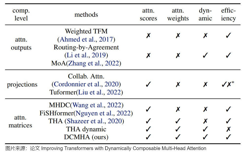
The source comparison separates composition at projected features, attention scores/weights, or head outputs. That axis is more useful than comparing names.
MOHSA: overlap projected head channels
Multi-Overlapped-Head Self-Attention starts from the observation that standard head slices are disjoint. It gives a head access to overlapping channel ranges from adjacent heads before attention, then projects the enlarged head representation back to the intended dimension.
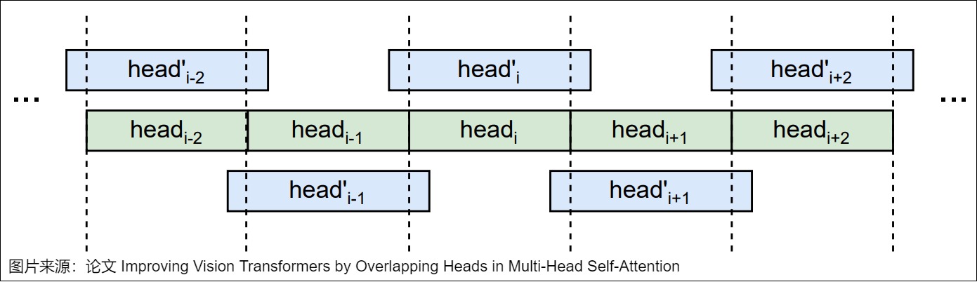
The changed object is the head partition:
classic:
    head_i = projected[..., i*d_head:(i+1)*d_head]

overlapped:
    head_i reads its core slice plus bounded adjacent-head channels
This creates feature exchange before score construction. It does not route tokens to a subset of heads and it does not share K/V across query heads. The paper evaluates a Vision Transformer setting, so transferring its result to language-model training or serving is an empirical question, not a consequence of the layout alone.
Runtime integration also differs from classic view(...).transpose(...).
Simple slicing may create overlapping views, but the enlarged per-head width,
padding at boundary heads, and reduction projection need checkpoint and kernel
support. A source-level implementation cannot claim the same cost from the old
h*d_head=d_model ledger without counting those operations.
The more detailed A12 figure makes the changed tensor visible:
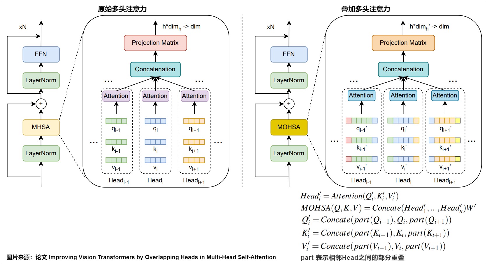
Let classic head width be D and let each interior head borrow r channels
from each adjacent head. Its attention width becomes:
for interior heads, with a documented boundary policy for the first and last
heads. If all H heads use width D', pairwise score work scales from:
to approximately:
The concat width becomes HD', so a reduction/output projection must map it
back to d_model. An implementation can construct overlap through views and
gathers, but overlapping logical channels mean the same projected feature may
participate in more than one head’s score/value computation.
A checkpoint conversion from classic MHA therefore needs answers to:
How are borrowed channels initialized?
Are the original core head slices copied exactly?
Is the reduction projection initialized to recover the old output?
How do boundary heads borrow channels?
Does the runtime materialize overlapped tensors or consume strided/gathered views?
MOHSA is architecture-compatible at the block interface, not automatically function-preserving at initialization.
Talking-Heads and DCMHA: compose score/probability heads
Talking-Heads Attention inserts learned linear projections across the head axis before and after softmax. If classic score tensor is:
S: [B,H_q,Q,K]
a pre-softmax head projection mixes S[:, :, i, j] across heads for every
query-key pair; a second projection mixes the normalized attention weights.
Token axes remain Q x K, but heads are no longer independent during routing.
Using the Talking-Heads paper’s distinction, projected Q/K can create
H_k logit heads, a pre-softmax matrix maps them to H softmax heads, and a
post-softmax matrix maps them to H_v value heads:
The head-mixing parameter count is:
small relative to d_model^2 for ordinary head counts. But the operation is
applied at every query-key pair, so activation work scales with BQK times
those head-axis products. Parameter count alone understates runtime cost.
DCMHA generalizes head composition by making parts of the composition input-dependent. Its core distinction is not “more virtual heads” as a literal stored tensor. It transforms score and weight matrices with compose functions conditioned on Q/K, including low-rank/dynamic components intended to control cost.
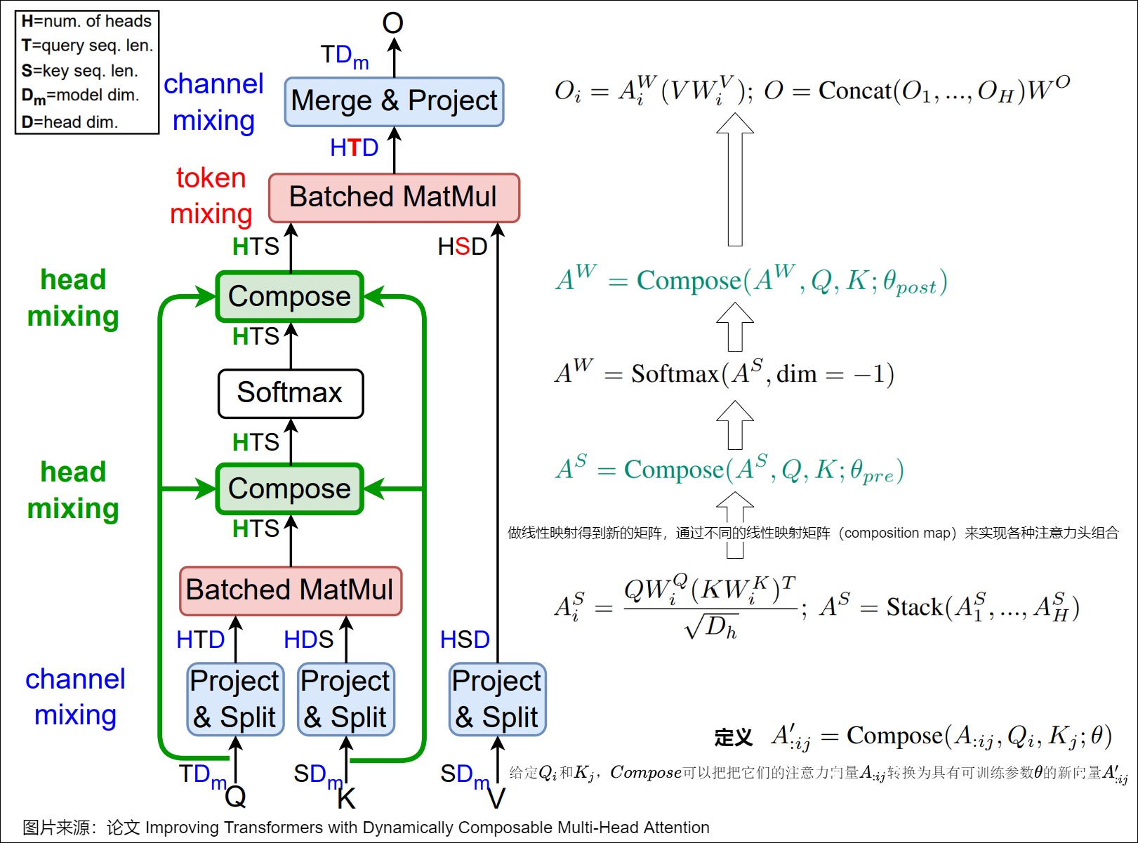
This placement matters mathematically:
compose before softmax:
    changes logits and therefore the normalized routing distribution

compose after softmax:
    mixes already-normalized per-head routing weights

W_O after value mixing:
    mixes output channels, not attention score matrices
Classic W_O cannot generally reproduce pre-softmax composition because
softmax is nonlinear. Mixing outputs after P_h V_h is not equivalent to
mixing the logits before each P_h is formed.
DCMHA can be read as a query/key-conditioned head-mixing matrix for each token
pair. For attention vector A_ij in R^H, the source article summarizes the
composition as:
with:
The dynamic query and key terms are further represented with low-rank and
diagonal components so the model does not generate a dense unconstrained
H x H matrix independently for every pair.
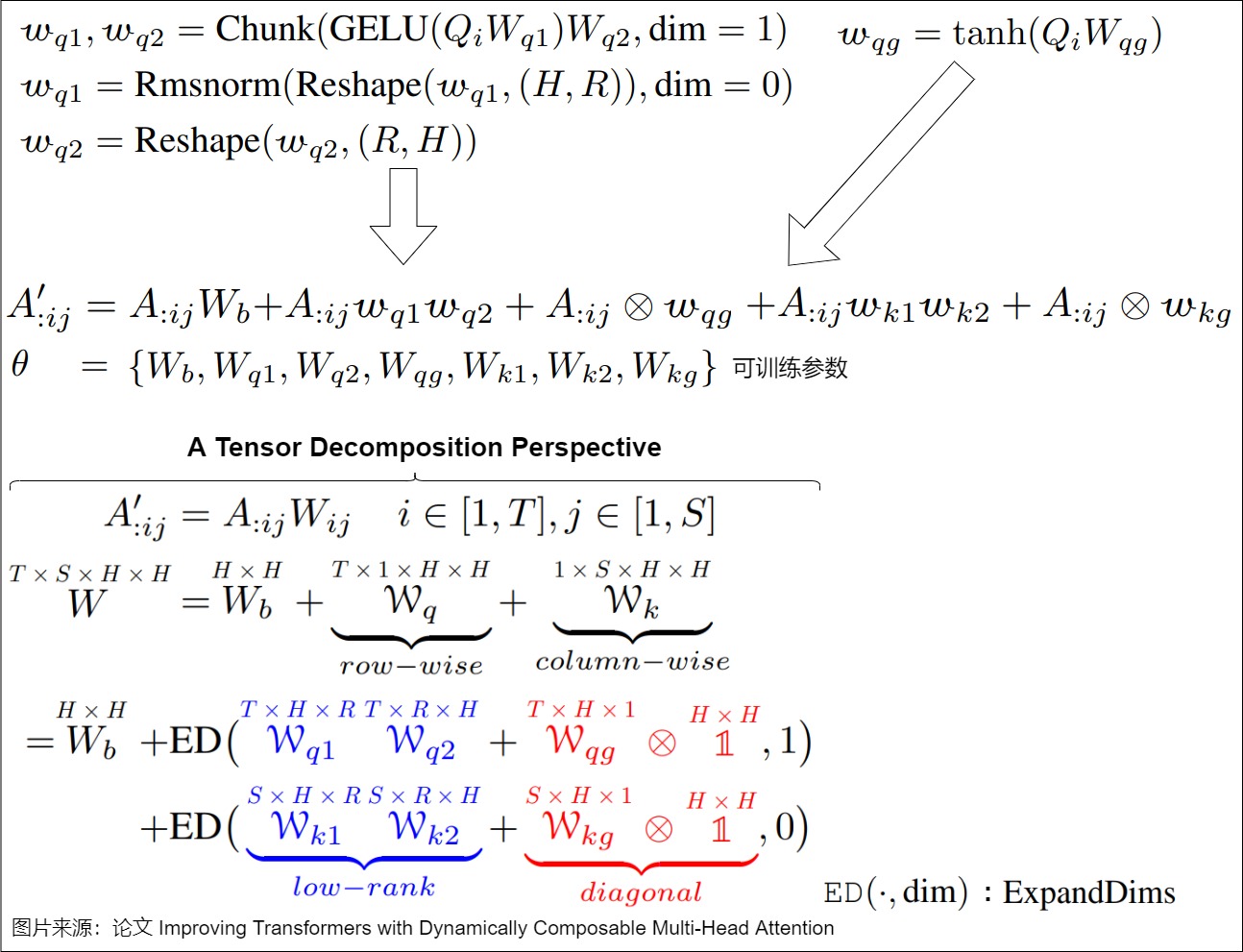
The detailed process figure exposes where those terms enter one attention vector:
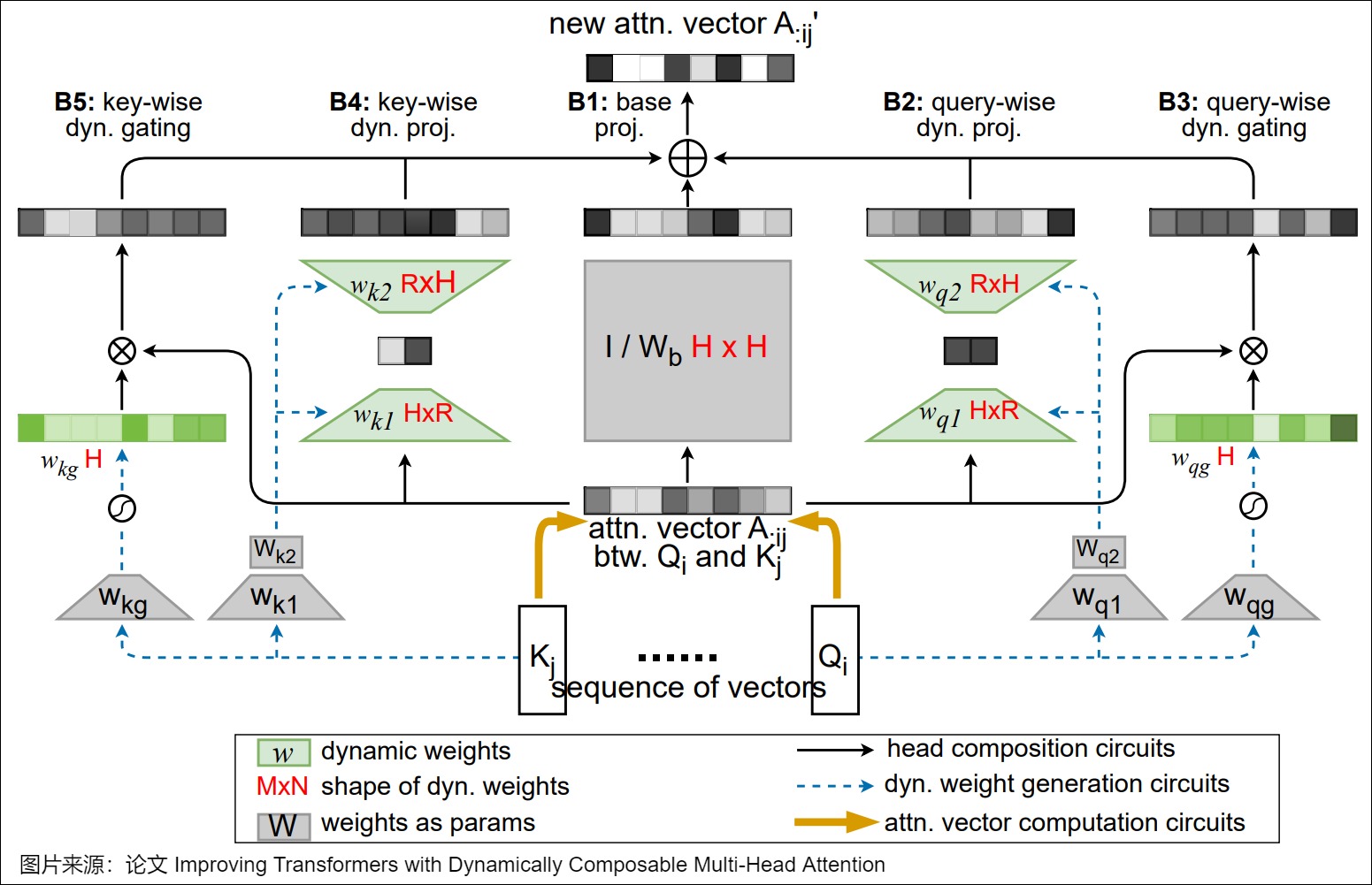
This decomposition creates several implementation contracts absent from classic MHA:
generate query-conditioned low-rank factors and gates;
generate key-conditioned low-rank factors and gates;
normalize or constrain dynamic factors as specified;
compose the head vector before/after softmax at the intended locations;
avoid materializing a full [B,Q,K,H,H] tensor;
differentiate through dynamic weights and attention values.
A naïve implementation that materializes [B,Q,K,H,H] can erase the intended
efficiency even if the paper’s factorized formula is inexpensive.
These variants add training and integration state: composition parameters, possibly input-conditioned low-rank projections, initialization rules, and kernel work on the head axis. Claims that they are drop-in at the architecture level do not guarantee a drop-in fused kernel or checkpoint conversion.
MoH: route tokens through selected heads
Mixture-of-Head Attention treats heads as conditional experts. Its source architecture keeps shared heads that are always active and routed heads selected according to token-dependent router scores.
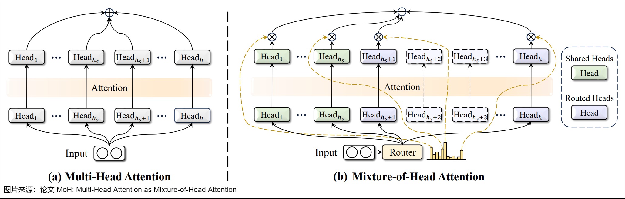
A conceptual output is:
A12 also retained the routing and balancing equations from the source paper:
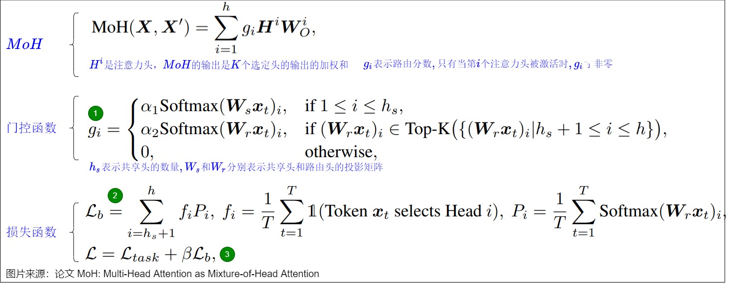
For routed heads, define assignment frequency f_h and average router
probability p_h over T tokens. The MoH paper’s routed-head balancing term
uses the unscaled sum:
and the total training objective becomes:
Other routed architectures may multiply an equivalent statistic by the number of experts or heads, so the normalization must follow the paper or implementation being reproduced. The purpose of the auxiliary term is not to make every token use every head. It discourages collapse in which a few routed heads receive nearly all assignments.
The changed choice is “every head runs for every token.” Routing introduces additional contracts:
router input and score calculation
shared-head count
top-k routed-head selection
gate normalization / weighted merge
load-balancing objective
sparse execution support
Skipping head outputs in mathematical notation does not automatically reduce latency. A dense implementation that computes all heads and masks most outputs saves no attention arithmetic. Real efficiency requires kernels and layouts that avoid work for inactive token-head pairs without losing the savings to sorting, dispatch, irregular shapes, or synchronization.
Training has an additional distinction: top-k selection is discrete, but the selected head outputs and router scores still need useful gradients. Practical implementations differentiate through selected gates and add balance pressure; they do not receive gradients for arbitrary unselected head computation in the same way as dense MHA. Router initialization, tie handling, capacity, shared head count, and load telemetry are part of the model contract.
MQA/GQA: share K/V rather than compose or route query heads
MQA and GQA alter a different axis. Query heads remain numerous, while fewer K/V heads are projected and cached:
classic MHA: H_q = H_kv
GQA:         H_q > H_kv > 1
MQA:         H_kv = 1
Their main serving benefit comes from reducing K/V projection and cache state, not from dynamically selecting query heads. M5.7 owns the complete cache and kernel analysis.
Variant comparison ledger
| Variant | Changed object | Token-dependent? | Extra training state | Primary runtime question |
|---|---|---|---|---|
| classic MHA | none; independent head slices | no | Q/K/V/O parameters | can packed projections and batched heads run efficiently? |
| MOHSA | projected channel partition overlaps | no | overlap/reduction parameters as designed | can overlapping slices and reductions be fused? |
| Talking-Heads | head-axis projections on logits/weights | no | pre/post softmax head-mixing matrices | what is the cost of head-axis mixing around softmax? |
| DCMHA | dynamic composition of score/weight heads | yes | static and input-conditioned compose parameters | can dynamic composition remain efficient at target scale? |
| MoH | active head set and weighted head merge | yes | router, shared/routed configuration, balance loss | does sparse head execution avoid inactive work? |
| GQA/MQA | K/V head count and sharing map | no | changed K/V projection/checkpoint layout | how much K/V memory and bandwidth is saved? |
Variant parameter and activation ledger
The table above identifies semantics. A second ledger identifies what must be counted before comparing efficiency:
| Variant | Additional parameter term | Additional/changed activation term | Can classic packed kernel run unchanged? |
|---|---|---|---|
| MOHSA | overlap reduction/projection as designed | wider or gathered per-head Q/K/V | no |
| Talking-Heads | H_k*H + H*H_v | head-axis transforms for every B*Q*K pair | no |
| DCMHA | static plus low-rank/gating generators | input-conditioned head composition; must avoid [B,Q,K,H,H] materialization | no |
| MoH | router plus shared/routed configuration | sparse token-head assignment and dispatch metadata | no, unless dense fallback |
| GQA/MQA | smaller K/V projections | fewer persistent K/V heads; query-to-KV group mapping | specialized or grouped path |
For H=32, a static 32 x 32 head-mixing matrix has only 1,024 parameters.
Applied to a dense Q=K=4096 attention tensor, however, one such transform is
conceptually repeated over more than 16 million token pairs per batch item.
Factorization and fusion are therefore runtime requirements, not secondary
optimizations.
Likewise, MoH with top-8 of 32 routed heads has a nominal active-head fraction
of 25 percent only if shared heads are counted separately and the backend
actually skips inactive Q/K/V, score, softmax, value, and output work. Reporting
k/H alone is not a latency model.
The comparison explains why head variants require separate evaluation. One method changes representation overlap, another changes routing interactions, another introduces conditional execution, and another compresses persistent K/V state. Their quality and speed claims are source-reported results under specific models and kernels; the mechanism does not guarantee the benchmark.
0x0BBA Paper-by-contract reconciliation of changed head programs
The preceding sections explain each idea. This section makes the comparison reproducible. The owner question is:
Given the same model-width input and output boundary, which tensor does each paper change, which new state must be trained or loaded, and which execution claim survives an implementation that merely computes the dense fallback?
The answer begins with one invariant. Every variant below can return a tensor
[B,Q,d_model], but equal outer shape does not mean equal internal program:
MOHSA:         changes projected feature membership before score construction
Talking-Heads: changes the head axis of logits and probabilities around softmax
DCMHA:         makes those head-axis transforms query/key conditioned
MoH:           changes which output-head branches are active for each token
MQA/GQA changes K/V ownership instead and remains an M5.7 handoff.
MOHSA contract: overlap coordinates, not tokens or attention maps
The MOHSA paper starts from hard channel partitions:
and constructs, for overlap width r on each side:
with analogous K'_i and V'_i. Therefore:
The first head has no i-1 neighbor and the last has no i+1 neighbor. The
paper uses zero padding for those missing sides so every head still has the
same enlarged width. That is a kernel-friendly rectangular contract; omitting
the pad would create ragged boundary heads.
The head output and final projection are:
The base Q/K/V projections need not grow: overlap can gather coordinates from
their existing H*D packed result. W'_O does grow. Relative to a classic
[HD,d_model] output matrix, its additional weight count is:
The score/value products also use D+2r instead of D. For self-attention,
the additional local MACs are approximately:
because both QK^T and PV gain 2r channels per head. The enlarged output
projection adds:
Gather/materialization traffic is separate. The same base coordinate can be
read by its core head and a neighbor; overlapping a view does not duplicate
checkpoint parameters, but a materialized [B,H,S,D+2r] tensor duplicates
activation elements.
Overlap schedules are architecture state
The paper evaluates more than one fixed r. It defines fixed overlap and
depth schedules that increase or decrease overlap dimensions, with zero- or
one-indexed endpoints. A checkpoint must therefore record one r_l per layer,
not only a global method name:
fixed-r:
    r_l = r for every layer

inc-0(x):
    starts at zero and increases by one every x layers

dec-1(x):
    decreases toward one under the declared layer indexing
These schedules and the paper’s quality results are source-reported for its ViT/CaiT/Swin experiments. They do not establish a language-model optimum.
Conversion choices
When r=0, MOHSA reduces exactly to classic MHA if W'_O=W_O. For r>0, the
borrowed Q/K coordinates already change the score and its softmax denominator,
while borrowed V coordinates change the value mixture. Zeroing only the new
rows of W'_O therefore does not preserve the classic function: the core
head output reaching the copied rows has already changed. Two conversion
choices answer different questions:
explicitly gated compatibility rewrite (not the paper architecture):
    keep the classic D-wide attention path intact;
    place the borrowed Q/K/V contribution behind a continuation gate eta;
    initialize eta=0, then open it during continued training

paper-style new architecture training:
    initialize the complete widened projection under the paper/training recipe;
    no exact base-checkpoint parity is implied
The first requires an additional functional decomposition: simply multiplying
the final borrowed output channels by zero is insufficient. It is a rewrite
option, not a claim that the MOHSA paper used that conversion. Boundary
padding, layer schedule, chosen side coordinates, attention scale for the
enlarged width, materialization strategy, continuation-gate state, and W'_O
initialization all belong in checkpoint metadata.
Talking-Heads contract: three head counts and two noncommuting maps
Talking-Heads separates three counts that classic MHA normally identifies:
H_k: Q/K heads that produce logits J
H_s: heads normalized by softmax
H_v: value/output heads consumed by V
Using batch and token axes explicitly:
J:    [B,Q,K,H_k]
P_l:  [H_k,H_s]
L:    [B,Q,K,H_s]
W:    [B,Q,K,H_s]
P_w:  [H_s,H_v]
U:    [B,Q,K,H_v]
V:    [B,K,H_v,D_v]
O:    [B,Q,H_v,D_v]
The exact sequence is:
P_l mixes logits before their key-axis denominator is formed. P_w mixes
probabilities after each softmax-head row has normalized. In general:
Moving P_l after softmax changes the function. Moreover, U is not required
to be a nonnegative row-stochastic probability tensor: an unrestricted P_w
can create signed values or row sums other than one. It is a learned linear
head-axis combination consumed by the value product, not a second softmax.
The two added parameter terms are:
They are small in checkpoint bytes, but are applied to every query-key pair:
The full scalar-multiplication formula in the paper, using source length m,
query length n, query/source widths d_X,d_M, and equal output/query width,
is:
This formula exposes two design choices hidden by H=H_k=H_s=H_v: more
softmax heads can be added without widening Q/K/value channels, and more Q/K or
value heads change the large projection/product terms. The paper evaluates
these dimensions separately; its benchmark results remain source-reported.
Identity matrices recover classic MHA only when the three head counts agree and the Q/K/value projections already have matching head order:
This is a useful conversion oracle. It is not proof that arbitrary learned
Talking-Heads checkpoints can be folded into W_O: pre-softmax mixing crosses
a nonlinearity and cannot generally be moved after value mixing.
DCMHA contract: factorized dynamic maps around the same denominator
DCMHA retains pre- and post-softmax head composition but conditions each compose operator on the current query row and key row. Let:
A:    [B,H,Q,K]       logits or post-softmax weights
Q_x:  [B,Q,d_model]   unprojected/model-width query state
K_x:  [B,K,d_model]   unprojected/model-width key state
R:    small dynamic rank; the paper uses R=2 in its main design
For one query-key pair, the conceptual map is:
Materializing every W_ij would require:
elements in addition to the attention tensor. DCMHA instead decomposes the map into query-row and key-column terms, each low-rank plus diagonal:
Here:
W_q1(i), W_k1(j): [H,R]
W_q2(i), W_k2(j): [R,H]
w_qg(i), w_kg(j): [H]
The resulting vector operation is:
The paper presents a static base W_b in the general derivation, then reports
that its practical design replaces that branch with the identity skip shown
above. Saying merely W_b+W_q+W_k hides this implementation choice.
Dynamic-weight generation
For each query or key row, a small FFN generates both low-rank factors. In the paper pseudocode:
model row [d_model]
    -> W_1 [d_model,2HR]
    -> GELU
    -> W_2 [2HR,2HR]
    -> split into two HR vectors
    -> reshape factors and RMS-normalize the first factor over heads

separate model-row projection [d_model,H]
    -> tanh
    -> diagonal gate
There are separate query and key generators, and separate parameter sets for pre-softmax and post-softmax compose. Across both compose locations, the added parameter count under this contract is:
The paper’s simplified extra-parameter ratio, assuming d_model=H D_h and
D_h >> 2R, is:
That is a paper-convention ratio against the declared Transformer-layer denominator, not a universal model-parameter percentage.
The paper uses small initial scales for the dynamic projection/gating generators because large dynamic terms destabilized training, with Xavier initialization for other DCMHA parameters. The identity skip makes a zero dynamic state exactly recover the uncomposed tensor; the paper’s small random initialization is near-identity, not bitwise checkpoint parity.
Order, masking, and tensor parallelism
The complete order is:
QK logits under the declared scale convention
  -> pre-compose(logits,Q_x,K_x)
  -> apply causal/additive mask
  -> softmax over key positions
  -> post-compose(probabilities,Q_x,K_x)
  -> value product
  -> merge and W_O
The paper pseudocode applies the causal mask after pre-composition and before
softmax; its algorithm display omits score scaling. Because scalar score
scaling commutes with an unmasked linear head composition but additive masking
does not, an implementation must freeze its scale placement and must preserve
the paper’s mask boundary. A runtime must not compose finite logits after
inserting -inf in a
way that creates NaN, and post-composition must not violate visibility when
different heads use different masks. The common shared causal/padding mask is
safe because composition changes only the head axis for the same (q,k) pair;
head-specific visibility requires an explicit re-mask or stronger proof.
In tensor-parallel training, the paper also evaluates grouped composition: each rank composes only its local head group. This avoids new cross-rank head communication but removes cross-group composition. “No added communication” therefore describes a different composition domain, not all-head equivalence by construction.
MoH contract: weighted head summation, two-stage routing, sparse execution
The direct-sum form from 0x09B lets MoH weight complete head contributions:
Define H_s shared heads and H_r=H-H_s routed heads. To avoid ambiguity
between total active heads and routed top-k, call the routed budget K_r in
this article. Then each token has:
head branches, unless a specific implementation defines its published K
to include shared heads.
For the paper’s trainable two-stage router, with token state
x_t in R^{d_model}:
All shared heads remain active. Routed heads are selected by top-k routed router logits. Their final gates are:
The strict router parameter ledger is:
before optional biases. This is small relative to the four dense attention matrices, but not literally zero. A paper table may round the total model size to the same number; an artifact manifest should keep the exact count.
The load-balance term applies to routed heads. With routed probability mean
P_i and assignment frequency f_i:
The paper reports beta=0.01 as its default. That coefficient and the exact
normalization are source-reported training choices, not laws of routed heads.
From-scratch and pretrained-conversion lanes differ
The paper does not use one universal router schedule:
| Lane | Shared heads | Router/weighting | Training contract |
|---|---|---|---|
| from-scratch MoH | configured always-active subset | trainable shared, routed, and head-type projections plus balance loss | train the architecture and router jointly for the target model/task |
| LLaMA3-8B conversion in the paper | first 16 heads of each layer selected as shared | parameter-free query-head L2-norm routing; quantized forward head-selection score with straight-through gradient | first adapt the original model to available data, then convert and continue-train MoH |
The paper reports a two-stage 300B-token data-adaptation phase followed by a 100B-token MoH phase for that LLaMA3 experiment. Those figures describe the paper’s conversion, not a minimum recipe. They do show that a randomly inserted router and continuously reweighted outputs are not automatically a function-preserving checkpoint edit.
Active notation is not sparse execution
A dense fallback can compute all H heads and multiply unselected outputs by
zero. It preserves the mathematical mixture but retains dense work. The MoH
paper’s source-reported timing experiment instead constructs sparse Q/K/V
features from the router mask and replaces matrix multiplications with sparse
matrix multiplications under its test setup.
A complete runtime record must say which stages are skipped:
Q/K/V projection coordinates
QK score products
mask and softmax rows
probability-value products
W_O head blocks
router sort/gather/scatter and sparse metadata
Skipping only W_O blocks is not the paper’s full active-head arithmetic
claim. Conversely, per-token Q/K/V sparsity interacts with pairwise attention:
query and key tokens may select different heads. A kernel must define the
resulting token-head visibility and sparse pair layout; the weighted output
equation alone does not provide that implementation.
Executable changed-object comparison
The article’s variant oracle fixes one small tensor program for each paper:
MOHSA:
    builds zero-padded adjacent overlap, proves r=0 classic parity,
    and counts widened W_O plus activation coordinates

Talking-Heads:
    executes H_k -> H_s -> H_v, proves identity-map classic parity,
    and demonstrates pre/post-softmax noncommutativity

DCMHA:
    matches factorized low-rank-plus-diagonal compose to an explicit HxH oracle,
    proves zero-dynamic identity, and records the forbidden dense map size

MoH:
    executes shared/routed/type gates, verifies exactly H_s+K_r active branches,
    computes routed load balance, and records dense runtime as unmeasured
These fixtures establish tensor semantics and accounting. They do not reproduce paper training runs, quality measurements, fused kernels, or sparse speedups.
Changed-program failure lab
| Failure | Shape-compatible symptom | Required guard |
|---|---|---|
| MOHSA omits boundary padding | first/last head widths differ or are silently narrowed | one fixed D+2r contract with zero-filled missing neighbor |
| MOHSA counts overlap as free view state | checkpoint count looks small while activation/work grows | separate shared source coordinates from gathered/materialized activations |
MOHSA zeros only borrowed W'_O rows and claims checkpoint parity | output shape and copied rows look correct, but Q/K denominators and V mixtures changed earlier | exact parity only at r=0, or use an explicit gated classic-plus-overlap rewrite |
Talking-Heads uses one H everywhere | equations run only for one configuration | explicit H_k, H_s, and H_v axes |
move P_l after softmax | output rank remains valid | noncommutativity oracle at fixed inputs |
call post-mixed U a probability | key rows can sum differently or become signed | label it a linear weight tensor, not an independently normalized distribution |
DCMHA materializes [B,Q,K,H,H] | exact output but explosive memory | factorized oracle plus materialization rejection ledger |
DCMHA composes after inserting -inf | shape is valid; arithmetic can become NaN | pre-compose finite logits, then apply mask at the declared boundary |
| grouped DCMHA claimed equal to all-head composition | local shapes match | record head-group domain and missing cross-group paths |
MoH reports only K_r/H active | shared heads disappear from ledger | report (H_s+K_r)/H and router work |
| MoH dense mask called sparse speedup | output matches mixture | name skipped stages and profile actual sparse execution |
| from-scratch router attributed to converted LLaMA | method name matches | freeze training-lane-specific router and initialization contract |
0x0BBB Source-audit recovery: Collaborative MHA and publication evidence
The publication source audit found one mechanism in A12 that was not redundant with the four contracts above: Cordonnier et al.’s Collaborative Multi-Head Attention, or CollabHead. Its owner question is:
Can heads share a learned Q/K feature basis while retaining head-specific score geometry, value projections, and output blocks?
The answer changes neither the token axes nor the final concat/W_O boundary.
It changes how Q/K score features are allocated across heads.
Shared Q/K basis and per-head metric
Let source and query rows have width D_in, let D_k=H*d_k be classic MHA’s
total Q/K projection width, and choose a shared width D_tilde. CollabHead
learns:
For head i, its unnormalized score matrix is:
Equivalently, m_i defines a head-specific diagonal bilinear metric over one
shared projected basis. Values and output blocks remain head-specific:
The title “collaborate instead of concatenate” must therefore not be read as
removing output concatenation. Collaboration occurs in the shared Q/K feature
basis; the paper’s output still concatenates value-head results before W_O.
Stack the mixing vectors as rows:
Classic MHA is a special case at D_tilde=D_k: concatenate the classic
per-head Q and K matrices into the shared matrices, and make row i of M a
block indicator with ones only on head i’s d_k coordinates. The executable
oracle recovers all classic score matrices exactly under that construction.
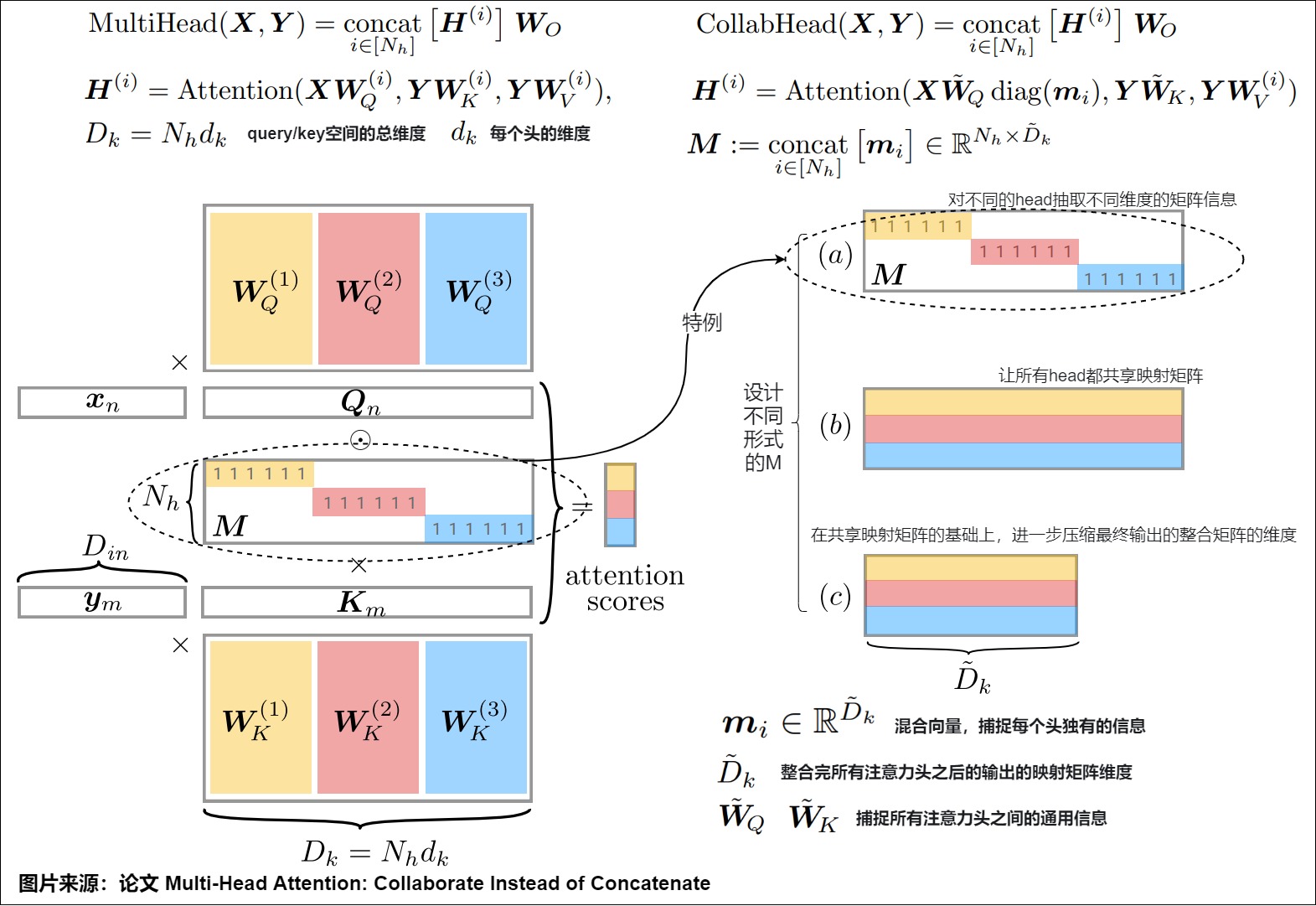
Upstream: Cordonnier et al., Multi-Head Attention: Collaborate Instead of Concatenate, Figure 2 and equations 7-9; the retained asset adds A12 annotations. The alternatives on the right are Q/K sharing designs, not evidence that a compressed conversion is exact.
Parameters, work, and conversion are separate contracts
Ignoring biases, classic Q/K projections contain:
parameters. Collaborative Q/K state contains:
including the mixing matrix M. W_V and W_O are unchanged, so this is not
the same intervention as removing complete heads. For self-attention with T
rows, the paper’s scalar-work convention gives:
Reducing parameter bytes does not guarantee a latency reduction: the shared projection, per-head metric, score product, layout, and target kernel determine execution. The paper’s timing and quality tables are source-reported results for its hardware, implementations, datasets, and dimensions.
The paper supports two training lanes:
from scratch:
    learn W_Q_tilde, W_K_tilde, M, per-head W_V, and W_O jointly

post-hoc conversion:
    stack the trained per-head products W_Q_i W_K_i^T
    -> factor the third-order [H,D_in,D_in] tensor
    -> obtain a shared Q basis, shared K basis, and mixing matrix
    -> retain bias correction state
    -> optionally fine-tune under the converted architecture
The paper uses a CP/PARAFAC-style factorization and records a per-head bias
correction vector when converting biased projections. Full shared width can
represent the classic construction exactly; compression to smaller
D_tilde is an approximation whose error and downstream recovery must be
measured. “Drop-in outer shape” is not “lossless compressed checkpoint.”
Five changed-head programs now have disjoint names
| Method | Changed object | Shared state | Input-conditioned? | Efficiency condition |
|---|---|---|---|---|
| CollabHead | Q/K feature basis and per-head diagonal metric | shared Q/K projections | mixing vectors are learned parameters, not token routers | smaller D_tilde plus a suitable implementation |
| MOHSA | adjacent Q/K/V channel membership | neighbor coordinates | no | overlap work/materialization must be priced |
| Talking-Heads | head axis around softmax | learned dense head maps | no | added pairwise head-axis transforms must be affordable |
| DCMHA | head axis around softmax | factorized compose generators | yes, from query/key rows | do not materialize [B,Q,K,H,H] |
| MoH | complete output-head contributions | shared always-on heads plus routed heads | yes, token router | inactive work must actually be skipped |
Publication evidence and failure closure
The article uses four visual classes. Their status is semantic, not cosmetic:
| Visual class | Retained examples | Reading contract |
|---|---|---|
| primary-paper extract | Transformer Figures 2/3 | supports only the paper figure’s local architectural or empirical claim |
| primary-paper derivative | Clark, Voita, CollabHead, MOHSA, MoH, DCMHA figures with A12 annotations/footers | upstream paper is named; added annotations are not part of the primary paper |
| A4/A12 reconstruction | call graphs, calculation traces, packed implementation path | local teaching artifact, checked against source equations/code rather than treated as paper evidence |
| secondary-review context | MHA/KV diagrams from two reviews | orientation only; M4/M5 and primary/official sources own system claims |
Provenance does not establish redistribution rights. The evidence manifest records upstream work, derivative status, route, byte hash, and use; license or permission must be checked independently for any distribution context that requires it.
The omitted A12 images were not discarded by count:
12-01: basic MHA overview superseded by primary Figure 2 and the code trace
12-02: typography analogy; decorative rather than tensor evidence
12-04: team/expert analogy; adds no mechanism beyond the introduction
12-07: arithmetic-intensity sketch; M4 owns a derived and measured cost model
12-08: learned-head example superseded by the primary Transformer Figure 3 extract
12-09: BERT pattern montage superseded by 12-11 and the dependency examples
12-10: restored here because CollabHead changes a distinct tensor contract
12-12: restored because it adds source-reported dependency-relation evidence
12-13: restored because it exposes the paper-specific pruning trajectory
Finally, every executable guard has a publication role:
| Failure family | Article guard | Mechanical evidence |
|---|---|---|
| wrong caller, source, fused span, mask, dtype, or backend claim | immutable call manifest | valid/invalid projection-call bundle oracle |
| packed/per-head/checkpoint disagreement | explicit projection reconciliation | packed/per-head numerical oracle |
| same-shape axis or stride corruption | coordinate-coded split/merge trace | layout and storage oracle |
wrong W_O block, head permutation, or wrapper derivative | direct-sum and adjoint equations | wrapper finite-difference oracle |
| source/target ownership or rectangular-mask drift | cross-stream call trace | rectangular ownership oracle |
| stale, wrong-source, wrong-adapter, beam, rollback, or release state | cross-KV state machine | lifecycle transition oracle |
| API parity confused with backend admission | framework contract matrix | official-source runtime diagnostic |
| attention map promoted to causal importance or dense mask called pruning speed | evidence ladder and intervention transaction | gate/surgery oracle |
| changed-head methods collapsed by outer shape | paper-by-contract comparison | four-program variant oracle |
| CollabHead compressed conversion called exact | full-width block recovery versus bounded compression | collaborative-attention oracle |
| broken route, empty alt text, untracked image, or source class | publication manifest | source/visual/link publication validator |
The local-link manifest resolves article routes against Markdown source files, not against a stale deployment. External URLs identify source objects; this audit does not convert their current network availability into a timeless guarantee.
0x0C What M3.2 does not own
| Boundary | M3.2 imports | M3.2 does not re-teach |
|---|---|---|
| M3.1 | attention(query,key,value,mask,dropout) | score scaling, mask semantics, softmax, value mixing |
| M3.3 | optional position bias may enter the attention call | T5, Shaw, ALiBi, DeBERTa, TUPE |
| M3.4 | Q/K may be rotated after projection and before scoring in RoPE models | RoPE proof, pairing conventions, cache-position geometry |
| M3.6 | MHA output remains [B,q_len,d_model] for the next sublayer | FFN/MLP expansion, SwiGLU, capacity |
| M3.7 | attention module becomes a sublayer inside residual/norm wrapper | LayerNorm, residual stream, Pre-LN/Post-LN |
| M4.1 | local MHA parameter/MAC/element ledger | whole-model totals, optimizer state, HBM traffic, arithmetic intensity |
| M4.3 | a backend may consume the head-shaped logical tensors under stricter layout contracts | online-softmax proof, tile schedule, IO complexity, kernel backward, and hardware measurements |
| M5.7 | H_q versus H_kv as a boundary note | MQA/GQA serving and grouped cache layout |
| M5.8 | low-rank/latent representation as a boundary note | MLA cache state and absorbed execution |
M3.2 owns the head-layout and cross-attention execution contracts plus a bounded comparison of variants that change head composition. M4 and M5 still own their full kernel, memory, and serving evaluation.
0x0D Shape ledger
Classic Harvard MHA:
| Object | Shape | Notes |
|---|---|---|
| input query rows | [B,q_len,d_model] | caller may pass same tensor as key/value |
| input key rows | [B,k_len,d_model] | source memory for cross-attn |
| input value rows | [B,k_len,d_model] | same sequence length as key |
W_Q(query) | [B,q_len,d_model] | packed projection |
W_K(key) | [B,k_len,d_model] | packed projection |
W_V(value) | [B,k_len,d_model] | packed projection |
after view Q | [B,q_len,h,d_k] | split last width |
after view K/V | [B,k_len,h,d_k] | split last width |
after transpose Q | [B,h,q_len,d_k] | attention-ready |
after transpose K/V | [B,h,k_len,d_k] | attention-ready |
mask after unsqueeze(1) | [B,1,q_len,k_len] or compatible | shared over heads |
| attention scores | [B,h,q_len,k_len] | from M3.1 |
self.attn | [B,h,q_len,k_len] | attention probabilities |
head output x | [B,h,q_len,d_k] | output of M3.1 |
after x.transpose(1,2) | [B,q_len,h,d_k] | prepare concat |
after contiguous().view(...) | [B,q_len,h*d_k] | merged heads |
merged output before W_O | [B,q_len,d_model] | because h*d_k=d_model |
| final output | [B,q_len,d_model] | residual-stream width preserved |
Running example:
B       = 2
q_len   = 5
k_len   = 7
d_model = 512
h       = 8
d_k     = 64

query after split: [2,8,5,64]
key after split:   [2,8,7,64]
scores:            [2,8,5,7]
head output:        [2,8,5,64]
merged output:      [2,5,512]
0x0E Failure lab
Constructor and projection bugs
-
d_modelnot divisible byh. The model cannot split the projected width into equal heads. -
Forgetting that
self.linearshas four layers. The first three are Q/K/V projections; the last isW_O. -
Accidentally sharing Q/K/V projection weights. Self-attention may receive the same input tensor for Q/K/V, but it should still use different learned projections.
-
Treating heads as separate Python modules when the checkpoint expects packed matrices. Equivalent math is possible, but the parameter layout and checkpoint loading must match.
Shape and layout bugs
-
Splitting the sequence axis instead of the channel axis. Heads are slices of the projected channel width, not chunks of tokens.
-
Wrong
vieworder.[B,h,q_len,d_k]and[B,q_len,h,d_k]have the same number of elements but different axis meaning. -
Missing
transpose(1, 2)before attention. The attention function receives[B,q_len,h,d_k]and treats sequence/head axes incorrectly. -
Using
.view(...)after transpose withoutcontiguous()or an equivalent reshape. The rank may be right, but memory strides are wrong or PyTorch raises an error. -
Concatenating along the sequence axis. Heads should merge into channels, not add more token rows.
-
Using
q_lento reshape K/V in cross-attention. The-1dimension must be inferred separately for query, key, and value.
Mask and call-site bugs
-
Forgetting
mask.unsqueeze(1). A[B,T,T]mask may not broadcast over the head axis as intended. -
Unsqueezing the wrong axis. The mask broadcasts over sequence instead of heads, or it misaligns with query/key axes.
-
Applying a target causal mask to cross-attention. Cross-attention keys are source memory rows, not future target tokens.
-
Assuming every MHA call has square scores. Cross-attention uses
[B,h,T,S].
Attention and output bugs
-
Treating
self.attnas the module output.self.attnis the probability tensor; the module output is the value mix afterW_O. -
Forgetting
W_O. The concatenated head tensor has the right shape, but not the same learned transformation. -
Rotating or biasing in the wrong location. RoPE belongs after Q/K projection and before scoring. Relative bias belongs inside the score path. M3.2 only creates the projected/head-shaped objects.
-
Classic MHA assumptions in GQA/MQA code. Modern K/V head count may differ from query head count before repetition.
-
Assuming an equal-group GQA layout without checking divisibility. The common
group_size = H_q / H_kvmapping requiresH_q % H_kv == 0. -
Treating logical K/V sharing as mandatory physical cache duplication. Kernels can map query-head groups to shared K/V heads without storing repeated cache rows.
Interpretation and comparison bugs
-
Claiming every head must have a distinct interpretable role. Independent parameters permit specialization, but trained heads can be redundant or removable.
-
Increasing
hwhile holdingd_headfixed, then calling the comparison cost-neutral. Total attention width becomesh * d_head, so parameters and compute change with the head count. -
Comparing head counts without reporting
d_model,d_head, or the projection layout. The same value ofhcan describe different model widths and different capacity allocations.
0x0F Handoff
M3.2 has now built the attention sublayer’s local implementation object:
X_q, X_k, X_v
    -> packed Q/K/V projections
    -> head layout
    -> M3.1 attention call
    -> head merge
    -> output projection
    -> [B,q_len,d_model]
M3.6 opens the other main sublayer: the position-wise FFN/MLP, where each row is transformed across the channel axis.
M3.7 assembles attention and FFN into a block:
residual stream
    -> norm / attention / dropout / residual
    -> norm / FFN / dropout / residual
M4.1 receives M3.2’s objects as countable tensors:
W_Q, W_K, W_V, W_O
Q/K/V activations
score and probability tensors
attention output and merged output
M3.2 defines the layout. M4.1 prices it.
The parallel multimodal checkpoint is X1.2. It reuses the query, key, value, head-layout, and cross-attention contracts from this article while comparing prefix fusion, learned-query resampling, and external media memory.
0xFF References
- M3.1 — Scaled Dot-Product Attention and Masks
- M3.6 — Dense and Gated MLPs
- M3.7 — Residual Stream, Normalization, and Block Assembly
- Exploring the Transformer Series (10) — Self-Attention
- Exploring the Transformer Series (11) — Mask
- Exploring the Transformer Series (12) — Multi-head Self-Attention
- M3.3 — Positional Geometry and Attention Bias
- M3.4 — Rotary Position Embedding
- M4.1 — Transformer Cost Model
- M4.3 — IO-Aware Attention, Online Softmax, and FlashAttention
- M5.7 - MQA and GQA
- M5.8 - MLA Latent Cache and Absorbed Kernels
- X1.2 - Multimodal Encoders, Projectors, Resamplers, and Fusion
- Vaswani et al., Attention Is All You Need
- Michel et al., Are Sixteen Heads Really Better than One?
- Voita et al., Analyzing Multi-Head Self-Attention: Specialized Heads Do the Heavy Lifting, the Rest Can Be Pruned
- Clark et al., What Does BERT Look At? An Analysis of BERT’s Attention
- Cordonnier et al., Multi-Head Attention: Collaborate Instead of Concatenate
- Shazeer et al., Talking-Heads Attention
- Zhang et al., Improving Vision Transformers by Overlapping Heads in Multi-Head Self-Attention
- Jin et al., MoH: Multi-Head Attention as Mixture-of-Head Attention
- Xiao et al., Improving Transformers with Dynamically Composable Multi-Head Attention
- The Annotated Transformer
- PyTorch 2.13,
torch.nn.MultiheadAttentionandscaled_dot_product_attention - Official Collaborative Attention implementation
- Official DCFormer implementation
- Official MoH implementation
- Hugging Face Transformers
v5.13.1,repeat_kvand LLaMA attention