M3.6 — Dense and Gated MLPs: Channel Mixing, Training, and Runtime

0x00 Overview And Background

M3.1 opened the attention score path. M3.2 wrapped that path in Q/K/V projections, head layout, concatenation, and the output projection.

The attention sublayer returns model-width state rows:

X_attn: [B, S, d_model]

Those rows have already exchanged information across the sequence axis. The other main Transformer sublayer performs a different operation:

attention:
    mixes information across sequence positions

FFN / MLP:
    transforms channels inside each position independently

The local object in M3.6 is therefore:

X: [B, S, d_model]
    -> expand each row to d_ff
    -> apply a nonlinear or gated transformation
    -> contract each row back to d_model
Y: [B, S, d_model]

The sequence length does not change. The batch size does not change. No token row reads another token row inside this dense FFN call.

---

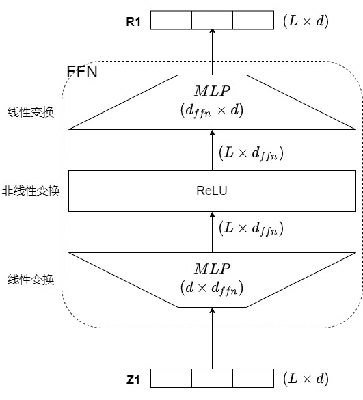
How the two-line FFN became a three-projection gated MLP

The MLP did not enter the Transformer as a mysterious store of facts. In the 2017 architecture it had a narrower engineering purpose: after attention had mixed sequence positions, every position received the same two-layer nonlinear map. The paper fixed the base-model widths at 512 -> 2048 -> 512, used ReLU, and described the two affine operations as kernel-size-one convolutions. That last description is another way of stating the position-wise contract: a kernel of width one transforms channels but has no neighboring token in its receptive field.

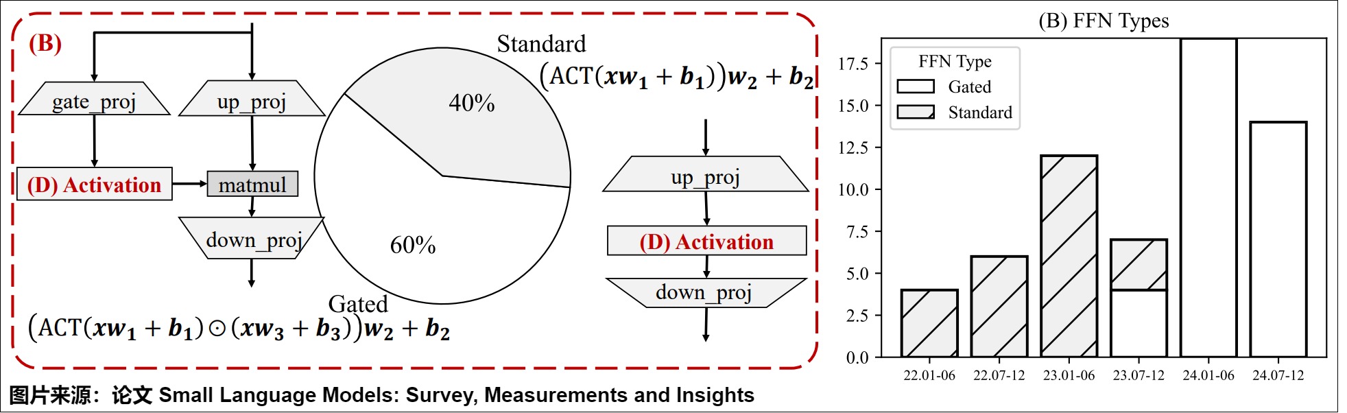
The later gated path came from two earlier lines of work that should not be collapsed into one chronology:

activation line:
    ReLU -> GELU / Swish / SiLU
    changes the scalar nonlinearity applied to one projected tensor

gating line:
    GLU -> ReGLU / GEGLU / SwiGLU
    adds a second projected branch and an elementwise product

Dauphin et al. introduced the gated linear unit for convolutional language models in 2016. The gate was an affine projection passed through a sigmoid and multiplied by a second affine projection. GELU was also proposed in 2016, while the Swish search paper followed in 2017. None of those papers by itself defines the modern LLaMA MLP. Shazeer’s 2020 GLU Variants Improve Transformer is the bridge: it replaced the sigmoid gate with ReLU, GELU, Swish, or even the identity, installed those variants in the Transformer feed-forward sublayer, and compared them after reducing the gated hidden width so the extra input projection did not receive an unacknowledged parameter and operation advantage.

PaLM later adopted SwiGLU as an architecture choice. LLaMA followed the same family while making the implementation contract especially visible: two bias-free input projections, a SiLU gate, one elementwise product, one down projection, and an intermediate width derived from the historical 4d width then rounded for alignment. Those choices are lineage, not a universal rule for every model calling itself “LLaMA-like.” The checkpoint and its implementation remain authoritative.

Step	Paper-level object	What actually changed	What did not follow automatically
original Transformer	position-wise ReLU FFN	two affine maps with one scalar nonlinearity	no gate branch
GLU	value projection times sigmoid gate projection	second input projection and multiplicative control	not yet a Transformer MLP
GELU / Swish	alternative scalar activations	response and derivative geometry	no extra projection by themselves
Transformer GLU variants	ReGLU, GEGLU, SwiGLU	gate activation plus matched-width experiments	no universal winning width or activation
PaLM / LLaMA lineage	large-scale SwiGLU decoder MLP	concrete bias, width, rounding, and naming policies	no guarantee that another checkpoint shares those policies

This history is operational. Replacing ReLU with GELU can preserve the two weight tensors. Replacing a ReLU FFN with SwiGLU adds another learned matrix and changes the hidden width, backward graph, packed-checkpoint layout, fusion contract, and tensor-parallel shard map. A configuration field named activation is therefore insufficient to reconstruct the latter.

Evidence and terminology contract

M3.6 uses four evidence levels throughout:

Label	Meaning in this article
architecture fact	follows from a primary equation, a checkpoint, or pinned official code
source-local	preserved from A2/A13 and labeled when not independently established
paper-specific result	observed under the named paper’s models, data, and evaluation
interpretation	a derived lens that helps reason about the graph but is not a universal empirical fact

The names FFN and MLP are used for the same per-token sublayer when context makes the topology explicit. Dense MLP means every token evaluates the local matrices. Gated MLP means two projected branches interact multiplicatively. MoE is not a synonym for gated MLP: it selects among multiple expert MLPs and belongs to M6.

Background knowledge: the block alternates token mixing and channel mixing

Attention is linear value mixing once its weights are fixed. A Transformer also needs a nonlinear transformation that can create, suppress, and recombine features inside each row. The original architecture used the same two-layer feed-forward network independently at every position.

attention:
    communicates across the sequence axis

FFN or MLP:
    expands and transforms the channel axis per row

residual wrapper:
    returns both operations to the common d_model stream

Modern gated MLPs such as SwiGLU change the activation path and parameter ledger, but not the basic ownership rule: they do not mix token positions. That separation becomes important later for FLOP accounting, tensor parallelism, MoE replacement, and failure diagnosis.

Owner question

Once attention has moved information between token rows, how does a Transformer create nonlinear features inside each row, how do dense and gated variants differ, and what state must training and inference actually materialize?

M3.6 owns more than the two-line Linear -> activation -> Linear mnemonic. It owns the derivation that prevents those two matrices from collapsing into one; the activation and gating design space; forward and backward tensor traces; parameter, compute, and activation-state ledgers; kernel and tensor-parallel integration; and the evidence behind interpreting intermediate channels as learned feature or memory directions.

It deliberately defers:

M3.7: residual paths, normalization, dropout around the sublayer, block order
M4:   whole-model cost, roofline, sharding, and kernel performance
M6:   routing among multiple expert MLPs
M8:   quantization, pruning, and compressed deployment of these matrices

Why the MLP exists at all

Suppose a block only stacked linear maps after attention. For one row, two affine maps compose as

$$f(x)=(xW_1+b_1)W_2+b_2 =x(W_1W_2)+(b_1W_2+b_2).$$

No matter how wide the intermediate tensor is, this composition remains one affine map. Width can factor the matrix, but it cannot introduce input-dependent feature selection. The nonlinearity or gate makes the intermediate response depend on the current row:

$$f(x)=\phi(xW_1+b_1)W_2+b_2.$$

This is why the MLP is not merely a parameter reservoir appended to attention. Attention supplies sequence-conditioned rows; the MLP applies a nonlinear basis expansion to each of those rows and maps the activated basis directions back into the residual stream.

0x01 The position-wise contract

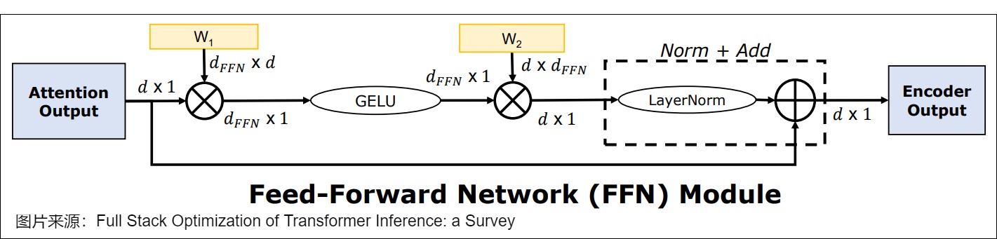
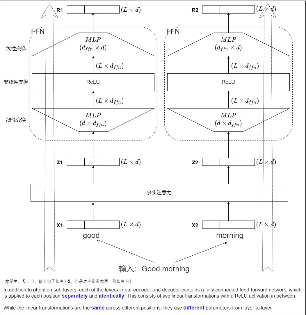
The original Transformer paper calls this a position-wise feed-forward network. The same learned function is applied separately and identically to every sequence position:

$$\operatorname{FFN}(x_i) = \max(0, x_iW_1+b_1)W_2+b_2$$

For a full tensor:

X: [B, S, d_model]

the operation is equivalent to flattening the batch and sequence axes into independent rows:

x_rows = x.reshape(B * S, d_model)
y_rows = ffn(x_rows)
y = y_rows.reshape(B, S, d_model)

This is a conceptual equivalence, not a requirement to reshape the implementation. nn.Linear already applies to the last dimension and preserves all leading dimensions.

The important contract is:

same parameters at every position in one layer
different FFN parameters in different Transformer layers
no reduction or mixing over S inside the FFN

For one output row:

y[b, i, :] depends on x[b, i, :]
y[b, i, :] does not directly read x[b, j, :] for j != i

The row can still contain contextual information gathered by attention. Position-wise does not mean context-free; it means the MLP does not perform another sequence-axis interaction.

Sequence permutation equivariance

The position-wise contract can be written as an algebraic invariant. Flatten one batch item to $X\in\mathbb R^{S\times d_{model}}$ and let $P\in\{0,1\}^{S\times S}$ permute its rows. Because the same affine maps and pointwise activation are applied to every row,

$$\operatorname{FFN}(PX) =\phi(PXW_1+\mathbf 1b_1^\top)W_2+\mathbf 1b_2^\top.$$

Permutation only reorders rows, so pointwise $\phi$ commutes with it:

$$\phi(PZ)=P\phi(Z).$$

Therefore

$$\operatorname{FFN}(PX)=P\operatorname{FFN}(X).$$

The MLP preserves a row permutation instead of discovering sequence order. Positional information can still be encoded inside each row by earlier operations, but the MLP has no independent sequence-axis adjacency rule.

This gives a useful test:

perm = torch.randperm(S)
y1 = mlp(x[:, perm, :])
y2 = mlp(x)[:, perm, :]
torch.testing.assert_close(y1, y2)

The test should run in evaluation mode or with synchronized dropout masks. A failure without stateful or token-coupled extensions usually means the implementation transformed the wrong axis.

Local Jacobian is block diagonal across token rows

If rows do not interact, the Jacobian with respect to flattened sequence state has block structure:

$$\frac{\partial\operatorname{vec}(Y)} {\partial\operatorname{vec}(X)} =\operatorname{diag}(J_1,J_2,\ldots,J_S),$$

where $J_i\in\mathbb R^{d_{model}\times d_{model}}$ is the channel Jacobian for row $i$. For a classic FFN under column-vector notation,

$$J_i=W_2^\top\operatorname{diag}(\phi'(W_1^\top x_i+b_1))W_1^\top.$$

Off-diagonal row blocks are zero. Attention has the opposite signature: changing one visible token can change another row through its attention weights and value mixture. This Jacobian distinction is more precise than saying only that “attention mixes tokens and MLP mixes channels.”

One function copied across rows, not one giant dense layer

Flatten $T=B\cdot S$ token rows into $X\in\mathbb R^{T\times d}$. The first affine projection can be written in vectorized form as

$$\operatorname{vec}(XW_1) = (W_1^\top\otimes I_T)\operatorname{vec}(X),$$

where $\otimes$ is the Kronecker product. The identity $I_T$ is the important object: the operator repeats the channel map for every row instead of learning connections between rows. Bias broadcasting contributes $\operatorname{vec}(\mathbf 1b_1^\top)$ and does not change that ownership.

This also makes the original paper’s kernel-size-one convolution statement exact. Treat each token row as one spatial location with d_model input channels. A one-dimensional convolution with kernel width one has weight [d_ff,d_model,1]; removing its singleton kernel axis gives the PyTorch linear weight [d_ff,d_model]. A wider convolution would couple neighboring sequence positions and violate the local MLP contract.

The equivalence has limits:

equivalent:
    same weight at every position
    kernel width exactly one
    matching bias and channel order

not implied:
    causal masking
    token neighborhoods
    padding semantics
    attention-like dynamic weights

Width, affine rank, and nonlinear regions

Without $\phi$, the effective channel matrix is $W_1W_2$ and

$$\operatorname{rank}(W_1W_2) \leq \min(d_{model},d_{ff}).$$

When $d_{ff}\ge d_{model}$, expansion does not let the collapsed affine map exceed rank $d_{model}$. The value of the hidden width is instead exposed by the intervening nonlinearity. For ReLU, define the row-dependent diagonal mask

$$D(x)=\operatorname{diag} \left(\mathbf 1\{xW_1+b_1>0\}\right).$$

Inside a region where this mask is fixed,

$$f(x)=(xW_1+b_1)D(x)W_2+b_2$$

is affine, but different input regions select different effective matrices $W_1D(x)W_2$. Increasing d_ff adds candidate boundaries and basis directions; it does not guarantee that training uses each channel, that each channel is interpretable, or that a particular width is optimal. Universal-approximation results concern function classes under assumptions about width, activation, domain, and approximation error. They are not a checkpoint-quality guarantee.

Gated Jacobian has two local gradient paths

For one bias-free gated row, let

$$G=xW_g,\qquad U=xW_u,\qquad H=\phi(G)\odot U,\qquad Y=HW_d.$$

Under row-vector differentials,

$$dH = dG\,\operatorname{diag}(U\odot\phi'(G)) + dU\,\operatorname{diag}(\phi(G)).$$

Substituting $dG=dxW_g$ and $dU=dxW_u$ gives the local channel Jacobian

$$J_{gated}(x) = \left[ W_g\operatorname{diag}(U\odot\phi'(G)) + W_u\operatorname{diag}(\phi(G)) \right]W_d.$$

The first term differentiates through the activated gate; the second through the linear value branch. Both depend on the same input row, so the Jacobian is input-dependent even when the activation is smooth. Across $T$ rows the global Jacobian is still block diagonal:

$$J_{global}=\operatorname{diag} \left(J_{gated}(x_1),\ldots,J_{gated}(x_T)\right).$$

This resolves two common misconceptions at once: gating creates richer local channel interactions, but it does not create token mixing. The accompanying finite-difference oracle perturbs one coordinate in one row and verifies both the analytic Jacobian and the zero cross-row response.

---

0x02 The classic two-matrix FFN code spine

A13 reconstructs the Harvard implementation:

class PositionwiseFeedForward(nn.Module):
    def __init__(self, d_model, d_ff, dropout=0.1):
        super(PositionwiseFeedForward, self).__init__()
        self.w_1 = nn.Linear(d_model, d_ff)
        self.w_2 = nn.Linear(d_ff, d_model)
        self.dropout = nn.Dropout(dropout)

    def forward(self, x):
        return self.w_2(self.dropout(self.w_1(x).relu()))

Read the forward path from the inside out:

x
  -> w_1(x)
    -> ReLU
      -> dropout
        -> w_2(...)

With shapes:

x:                  [B, S, d_model]
w_1(x):             [B, S, d_ff]
relu(w_1(x)):       [B, S, d_ff]
dropout(...):       [B, S, d_ff]
w_2(...):           [B, S, d_model]

This code owns the MLP transformation only. Residual addition and normalization are outside the class and belong to M3.7.

---

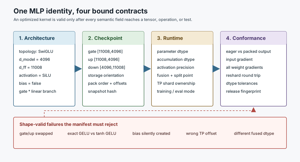
Immutable MLP, checkpoint, dtype, and runtime manifest

The code mnemonic is not enough to reproduce a trained MLP. A release needs an immutable manifest that binds each semantic choice to either a serialized tensor or an executable operation. At minimum, record:

Manifest group	Required fields	Why shape inspection alone fails
topology	dense or gated, projection count, branch equation	two [d_ff,d_model] tensors do not reveal which one is activated
widths	d_model, d_ff, alignment rule, width multiplier	a rounded width cannot be recovered reliably from a ratio
activation	exact function and approximation mode	exact GELU and tanh GELU share all tensor shapes
affine policy	bias per projection	missing biases can be silently initialized to zero
checkpoint layout	tensor names, storage orientation, separate/packed order	[gate; up] and [up; gate] are shape-identical
numerics	parameter, input, activation, accumulation, output dtypes	the same weights can drift or overflow under another compute path
stochastic state	hidden dropout probability and placement	moving a mask changes the trained function
parallel ownership	tensor-parallel degree, shard axis, global shape, rank order	local shards do not identify their global branch or offset
implementation identity	project, immutable revision, file and symbol	a moving main branch can change semantics after release

A compact SwiGLU manifest can look like this:

{
  "topology": "swiglu",
  "d_model": 4096,
  "d_ff": 11008,
  "activation": {"name": "silu", "beta": 1.0},
  "bias": false,
  "checkpoint": {
    "layout": "separate_pytorch_linear",
    "gate": "model.layers.{L}.mlp.gate_proj.weight",
    "up": "model.layers.{L}.mlp.up_proj.weight",
    "down": "model.layers.{L}.mlp.down_proj.weight"
  },
  "numerics": {
    "parameter_dtype": "bfloat16",
    "gemm_accumulation": "implementation_defined",
    "activation_compute": "implementation_defined"
  },
  "tensor_parallel": {"degree": 1, "intermediate_shard_axis": null},
  "implementation": {
    "project": "transformers",
    "revision": "4626421dc6b741a329300682a6408246ee465490",
    "symbol": "LlamaMLP"
  }
}

implementation_defined is an explicit unresolved field, not permission to assume FP32. A production release should replace it with the selected kernel’s contract and test tolerance.

Source-to-tensor trace: separate and packed implementations

The pinned Hugging Face Transformers revision used for this article constructs three nn.Linear modules and evaluates:

down_proj(act_fn(gate_proj(x)) * up_proj(x))

That gives these stored tensors under PyTorch’s [out_features,in_features] convention:

gate_proj.weight: [d_ff, d_model]
up_proj.weight:   [d_ff, d_model]
down_proj.weight: [d_model, d_ff]

The pinned Megatron-Core trace represents a different storage plan for the same local equation. When gated_linear_unit is enabled, linear_fc1 doubles its output width, the runtime chunks that last axis into x_glu and x_linear, and the checkpoint path uses stride-aware metadata so each half remains separately reshardable across tensor-parallel degrees:

logical branches:       gate [d_ff] + linear [d_ff]
materialized fc1 row:   [2 * d_ff]
chunk axis:             last activation axis
fc2 input:              gated product [d_ff]

The packed tensor is not simply “the same checkpoint with fewer files.” Its half order, global offsets, local shard order, and resharding factory are part of model identity. A correct loader proves equivalence on an input row before enabling fusion:

y_separate = down(silu(gate(x)) * up(x))

fc1 = linear_fc1(x)
gate_pre, linear = fc1.chunk(2, dim=-1)
y_packed = linear_fc2(silu(gate_pre) * linear)

torch.testing.assert_close(y_packed, y_separate)

The executable fixture accompanying this article checks tensor names, global shapes, parameter count, source revisions, and snapshot hashes. Later loops add numeric forward/backward and resharding oracles.

---

0x03 Expansion and contraction

The first projection expands the channel width:

self.w_1 = nn.Linear(d_model, d_ff)

The second projection returns to the residual-stream width:

self.w_2 = nn.Linear(d_ff, d_model)

The original Transformer used:

d_model = 512
d_ff    = 2048

so the row path was:

[512] -> [2048] -> [512]

For a batch of sequences:

[B, S, 512] -> [B, S, 2048] -> [B, S, 512]

The familiar d_ff = 4 * d_model ratio is an architectural choice from the original model, not a definition of FFN. Modern checkpoints choose intermediate_size according to architecture, parameter budget, hardware alignment, and whether the MLP has two or three projections.

Algebra shape versus PyTorch storage shape

With row-vector algebra, it is common to write:

W_1: [d_model, d_ff]
W_2: [d_ff, d_model]

PyTorch stores nn.Linear(in_features, out_features).weight as:

w_1.weight: [d_ff, d_model]
w_2.weight: [d_model, d_ff]

The forward operation internally uses the stored weight transpose. Mixing algebra notation with storage layout is a common checkpoint-conversion bug.

---

0x04 Why the nonlinearity matters

If the activation were removed, two affine transformations could collapse into one:

$$(xW_1+b_1)W_2+b_2 = x(W_1W_2)+(b_1W_2+b_2)$$

Expansion alone does not create a deeper nonlinear function. The activation between the projections changes the function class.

The classic path uses ReLU:

$$\operatorname{ReLU}(z)=\max(0,z)$$

Other model families use GELU, SiLU, or a gated activation. The activation name is part of the checkpoint contract:

same weight shapes + different activation = different model

The activation is not decorative. It changes sparsity, derivative flow, approximation error, and which fused kernels can implement the checkpoint. The local debugging questions are:

Which tensor is activated?
Where is dropout applied?
Does the checkpoint expect a simple activation or a gated branch?

ReLU: exact sparsity with a dead half-space

ReLU is piecewise linear:

$$\operatorname{ReLU}(z)=\max(0,z), \qquad \operatorname{ReLU}'(z)= \begin{cases} 0 & z<0,\\ 1 & z>0. \end{cases}$$

For an intermediate row $z=xW_1+b_1$, negative coordinates become exactly zero. That creates activation sparsity and an inexpensive derivative mask, but a coordinate that remains negative receives no local gradient through the activation. The convention at $z=0$ is framework-defined and has measure zero in ideal real arithmetic.

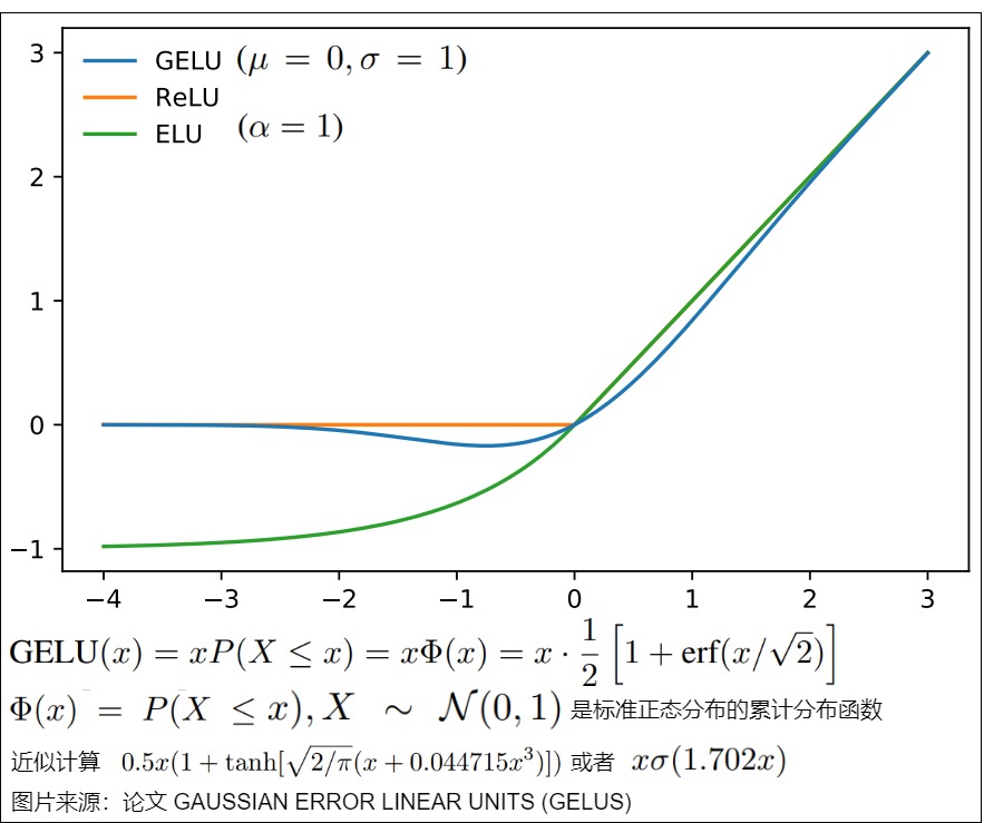
GELU: smooth input-dependent attenuation

GELU weights the input by the probability that a standard Gaussian variable is below it:

$$\operatorname{GELU}(z)=z\Phi(z) =\frac{z}{2}\left[1+\operatorname{erf}\left(\frac{z}{\sqrt{2}}\right)\right].$$

Its derivative follows from the product rule and $\Phi'(z)=\varphi(z)$:

$$\operatorname{GELU}'(z)=\Phi(z)+z\varphi(z),$$

where $\varphi$ is the standard-normal density. Unlike ReLU, GELU can preserve small negative responses and changes smoothly near zero. Implementations may use the exact erf form or a tanh approximation:

$$\operatorname{GELU}(z) \approx \frac{z}{2}\left[1+\tanh\left(\sqrt{\frac{2}{\pi}} \left(z+0.044715z^3\right)\right)\right].$$

Those variants share shapes but are not numerically identical. The approximation flag is part of the runtime contract when reproducing a checkpoint.

SiLU / Swish: a smooth self-gate

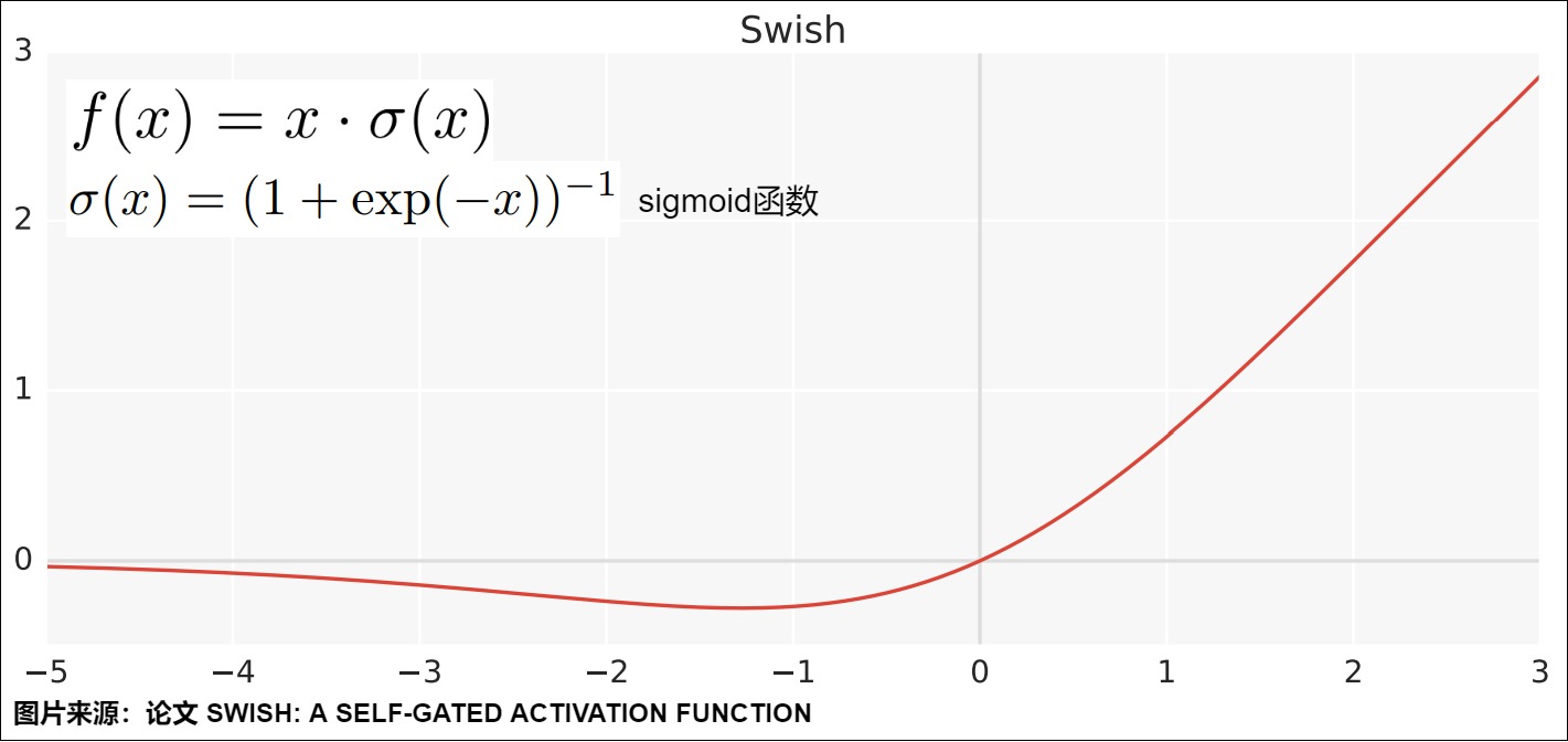
For the common fixed $\beta=1$ form,

$$\operatorname{SiLU}(z)=z\sigma(z), \qquad \sigma(z)=\frac{1}{1+e^{-z}}.$$

Differentiating exposes both paths through the self-gate:

$$\operatorname{SiLU}'(z) =\sigma(z)+z\sigma(z)(1-\sigma(z)).$$

SiLU is non-monotonic over a small negative interval and approaches the identity for large positive inputs. LLaMA-style SwiGLU uses this fixed activation; it does not add a separately learned $\beta$ unless the implementation explicitly declares one.

Numerical identity: names are not enough

An activation contract is a function, an approximation, and a compute policy. The string gelu is ambiguous unless the implementation also states whether it evaluates the Gaussian CDF or the tanh approximation. A commonly encountered third function, QuickGELU, is

$$\operatorname{QuickGELU}(z)=z\sigma(1.702z).$$

It resembles GELU but is neither the exact CDF definition nor the tanh approximation. Loading the same weights under those three functions changes the model without changing one tensor shape.

For the tanh approximation, define

$$q(z)=\sqrt{\frac{2}{\pi}}(z+0.044715z^3), \qquad t(z)=\tanh(q(z)).$$

Then

$$\widetilde{\operatorname{GELU}}(z)=\frac z2(1+t(z))$$

and its derivative is

$$\widetilde{\operatorname{GELU}}'(z) =\frac12(1+t(z)) +\frac z2(1-t(z)^2) \sqrt{\frac{2}{\pi}}(1+3\cdot0.044715z^2).$$

That derivative belongs to the approximated forward, not the exact GELU. Mixing an exact forward with an approximate custom backward fails gradient conformance even if inference logits look close.

The naive sigmoid expression 1 / (1 + exp(-z)) can overflow while computing exp(-z) for a large negative input. A stable scalar decomposition is:

def stable_sigmoid(z):
    if z >= 0:
        return 1.0 / (1.0 + exp(-z))
    ez = exp(z)
    return ez / (1.0 + ez)

Production vector kernels use equivalent range-safe transformations or hardware intrinsics. The contract is about the resulting function and tolerated error, not this branchy scalar implementation.

Function	$z\to-\infty$	$z\to+\infty$	Exact zeros	Local backward state
ReLU	output 0, derivative 0	output $z$, derivative 1	yes	sign mask or preactivation
exact GELU	output approaches 0 from below	approaches $z$	generally no	$z$ or sufficient recomputation state
tanh GELU	same limits, approximate middle	approaches $z$	generally no	approximation-specific $q,t$ or $z$
SiLU	output approaches 0 from below	approaches $z$	generally no	sigmoid/output or preactivation
QuickGELU	output approaches 0 from below	approaches $z$	generally no	its own scaled-sigmoid state

ReLU’s derivative at exactly zero is mathematically set-valued. Frameworks choose a convention; PyTorch uses zero. That convention rarely changes a continuous-distribution argument, but it matters for exact unit tests and quantized inputs that can land on zero frequently.

Dtype and fused-kernel contract

Four dtypes can differ in one activation path:

stored parameter dtype
GEMM accumulation dtype
materialized preactivation dtype
activation evaluation/output dtype

A reference implementation that promotes gate_pre to FP32 before SiLU and casts back is not numerically identical to a fused BF16 activation. FP16 has a narrower exponent range than BF16; BF16 has fewer fraction bits than FP16. Neither statement alone predicts which kernel is acceptable. The release must measure output and gradient error over the expected preactivation distribution, including tails, not just around zero.

The conformance matrix should include:

functions:
    ReLU, exact GELU, tanh GELU, SiLU, every supported fused variant

inputs:
    negative tail, transition region, positive tail, exact zero,
    non-contiguous tensors, odd row counts

checks:
    forward absolute/relative error
    derivative or VJP error
    NaN/Inf behavior
    deterministic mode where promised

The accompanying oracle evaluates exact and approximate formulas on a fixed grid, verifies their analytic derivatives by central differences, and records the approximation gap. The gap is not treated as a bug; selecting the wrong declared function is.

GLU is a two-branch layer, not a scalar activation

The original gated linear unit has two affine branches:

$$\operatorname{GLU}(x) =(xW_v+b_v)\odot\sigma(xW_g+b_g).$$

One branch proposes values and the other controls their passage. Replacing the sigmoid with another activation gives a family:

$$\begin{aligned} \operatorname{ReGLU}(x) &= \operatorname{ReLU}(xW_g)\odot(xW_v),\\ \operatorname{GEGLU}(x) &= \operatorname{GELU}(xW_g)\odot(xW_v),\\ \operatorname{SwiGLU}(x) &= \operatorname{SiLU}(xW_g)\odot(xW_v). \end{aligned}$$

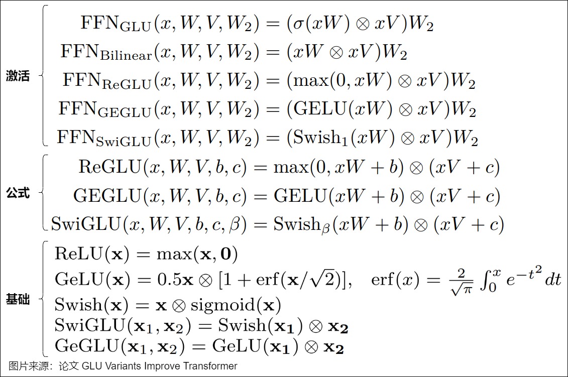
The naming rule describes the gate branch. Papers and libraries sometimes swap the letters used for gate and value matrices; the executable distinction is which branch receives the nonlinearity.

One generic graph, five distinct branch contracts

Write the complete gated FFN as

$$A=XW_g+b_g,\qquad V=XW_v+b_v,$$ $$H=\phi(A)\odot V,\qquad Y=HW_o+b_o.$$

The GLU family changes $\phi$, not the Hadamard product or the output projection:

Name in the 2020 paper	$\phi(A)$	Range/control consequence
GLU	$\sigma(A)$	bounded gate in (0,1)
Bilinear	$A$	no nonlinear gate; two linear branches multiply
ReGLU	$\max(0,A)$	exact zero gate on the negative half-space
GEGLU	$\operatorname{GELU}(A)$	smooth, signed small-negative gate
SwiGLU	$\operatorname{Swish}_1(A)$	smooth self-gate, usually implemented as SiLU

Only the sigmoid GLU has a gate constrained between zero and one. Calling the other branch outputs “gates” describes multiplicative modulation, not a probability or binary switch. ReGLU, GEGLU, and SwiGLU can amplify a coordinate; GEGLU and SwiGLU can also contribute a small negative coefficient.

Let $G_Y=\partial\mathcal L/\partial Y$. The complete generic backward is

$$G_{W_o}=H^\top G_Y,\qquad G_H=G_YW_o^\top,$$ $$G_A=G_H\odot V\odot\phi'(A), \qquad G_V=G_H\odot\phi(A),$$ $$G_{W_g}=X^\top G_A,\qquad G_{W_v}=X^\top G_V,$$ $$G_X=G_AW_g^\top+G_VW_v^\top.$$

The branches are therefore not symmetric when $\phi$ is nonlinear. Swapping gate and value preserves a bias-free Bilinear FFN because multiplication is commutative, but generally changes GLU, ReGLU, GEGLU, and SwiGLU. For ReGLU at $A_j<0$, both $\phi(A_j)$ and $\phi'(A_j)$ are zero, so that coordinate sends no local gradient into either input branch. Smooth gates have different negative tail behavior.

Variant ledger

Variant	Intermediate expression	Large matrices	Exact zeros	Runtime note
ReLU FFN	ReLU(xW1+b1)	2	yes	cheap mask; classic Transformer
GELU FFN	GELU(xW1+b1)	2	generally no	exact or approximate kernel
SiLU FFN	SiLU(xW1+b1)	2	generally no	not the same as SwiGLU
GLU	sigmoid(xWg+bg) * (xWv+bv)	3 with output projection	generally no	two input projections
ReGLU	ReLU(xWg) * xWv	3	gate-dependent	sparse gate branch
GEGLU	GELU(xWg) * xWv	3	generally no	common encoder-family choice
SwiGLU	SiLU(xWg) * xWv	3	generally no	common decoder-family choice

The GLU-variants paper reports empirical comparisons under matched parameter and compute budgets. Those results motivate the family; they do not establish that one activation dominates every architecture, data mixture, scale, precision, and kernel stack.

Paper and checkpoint lineage

Family	Local MLP form	Characteristic choice	Conversion question
original Transformer	Linear -> ReLU -> dropout -> Linear	two matrices, biases, $d_{ff}=4d$ in base model	where is hidden dropout stored?
BERT	Linear -> GELU -> Linear	smooth two-matrix FFN	exact or approximate GELU?
GPT-2	projection -> GELU variant -> projection	Conv1D storage convention	are stored matrices transposed relative to nn.Linear?
T5 v1.0	dense ReLU FFN	no bias in dense layers	is config relu or gated?
T5 v1.1 / gated variants	gated GELU-like branch	two input projections	which config/model revision owns the gate?
PaLM/LLaMA-style decoders	SwiGLU	bias-free in common checkpoints; reduced/rounded width	gate/up order and intermediate_size?

The table describes representative implementations, not every checkpoint carrying those family names. Architecture revision matters: “T5” or “LLaMA-compatible” is not enough information to reconstruct the MLP.

What the GLU-variants paper actually compared

The often-repeated statement “SwiGLU is better” compresses a specific study too aggressively. The 2020 paper used the T5 base transfer-learning setup:

architecture:
    encoder: 12 layers
    decoder: 12 layers
    d_model = 768
    attention heads = 12

matched MLP widths:
    two-matrix ReLU/GELU/Swish: d_ff = 3072
    three-matrix gated variants: d_ff = 2048

pretraining:
    C4 span-filling objective
    524,288 steps
    batch: 128 examples
    input length: 512 tokens
    output length: 114 tokens
    Adafactor + inverse-square-root schedule
    no dropout during pretraining in this experiment

At the final pretraining checkpoint, the paper reported this held-out log-perplexity on the span-filling task; lower is better:

Variant	524,288-step log-perplexity
ReLU baseline	1.677
GELU	1.679
Swish	1.683
GLU	1.663
Bilinear	1.648
ReGLU	1.645
GEGLU	1.633
SwiGLU	1.636

These are source-reported values from one matched T5-base training contract. The paper’s downstream fine-tuning results were noisy and different variants led different tasks; it did not provide a mechanism explaining the gains. Later adoption by PaLM, LLaMA, and other model families adds evidence that SwiGLU is practically useful, but it does not turn the table into a theorem about every decoder scale, optimizer, data mixture, precision, or kernel.

There are also three separate comparison questions:

equal intermediate width:
    isolates topology at higher gated parameter/compute cost

equal parameter/MAC budget:
    shrinks gated d_ff and compares different state widths

equal measured wall-clock budget:
    additionally depends on kernels, alignment, device, and parallel plan

The paper answers the second under its stated setup. M4 owns the third.

---

0x05 SwiGLU: two input projections and one output projection

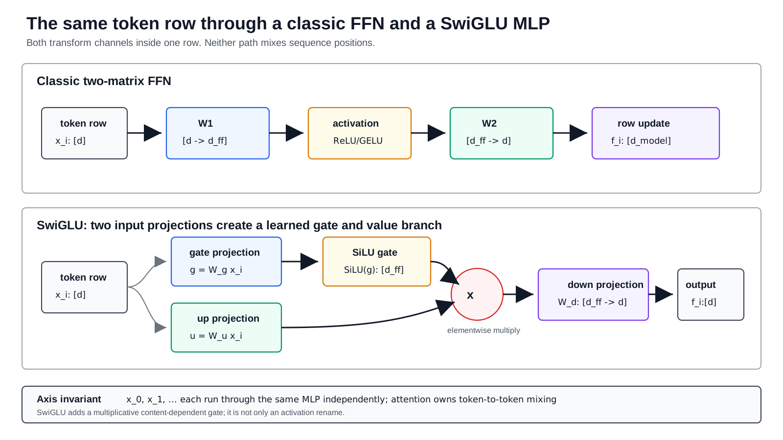
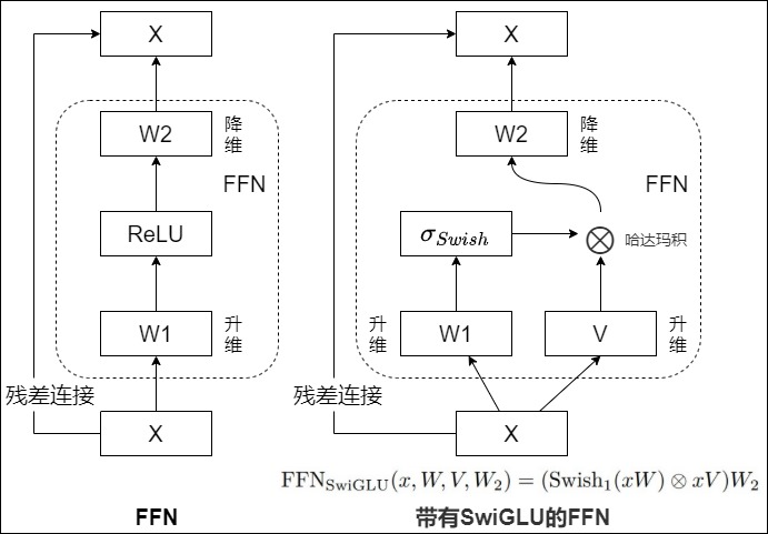
A gated MLP is not merely a classic FFN with ReLU renamed to SiLU.

The SwiGLU form in the GLU-variants paper is:

$$\operatorname{FFN}_{\text{SwiGLU}}(x) = \left(\operatorname{Swish}_1(xW)\odot xV\right)W_2$$

where odot is elementwise multiplication.

The local path is:

                     -> gate projection -> SiLU --+
x: [B,S,d_model]                               multiply -> down projection
                     -> up projection ----------+

Hugging Face Transformers v5.13.1 expresses the same LLaMA-style object directly:

class LlamaMLP(nn.Module):
    def __init__(self, config):
        super().__init__()
        self.hidden_size = config.hidden_size
        self.intermediate_size = config.intermediate_size
        self.gate_proj = nn.Linear(
            self.hidden_size,
            self.intermediate_size,
            bias=config.mlp_bias,
        )
        self.up_proj = nn.Linear(
            self.hidden_size,
            self.intermediate_size,
            bias=config.mlp_bias,
        )
        self.down_proj = nn.Linear(
            self.intermediate_size,
            self.hidden_size,
            bias=config.mlp_bias,
        )
        self.act_fn = ACT2FN[config.hidden_act]

    def forward(self, x):
        gated = self.act_fn(self.gate_proj(x)) * self.up_proj(x)
        return self.down_proj(gated)

Shape trace:

x:                     [B, S, d_model]
gate_proj(x):          [B, S, d_ff]
SiLU(gate_proj(x)):    [B, S, d_ff]
up_proj(x):            [B, S, d_ff]
elementwise product:   [B, S, d_ff]
down_proj(...):        [B, S, d_model]

Source-audit correction

A13 contains a conflicting shorthand that applies an additional sigmoid to the second branch. That is not the SwiGLU FFN used by the primary GLU-variants equation or the LLaMA implementation above.

The verified local contract is:

activated gate branch:
    SiLU(gate_proj(x))

linear value branch:
    up_proj(x)

gated intermediate:
    SiLU(gate_proj(x)) * up_proj(x)

In the GLU-variants paper’s Transformer experiment, Swish_1 fixes the Swish parameter to beta = 1. The default Hugging Face LlamaConfig uses hidden_act="silu", the x * sigmoid(x) activation. A learned beta is not present in the shown LlamaMLP contract.

Three implementation layouts that look similar but are not interchangeable

1. Separate projections keep gate_proj and up_proj as independent tensors and launch separate GEMMs.
2. Packed projection stores or constructs one [d_model, 2*d_ff] matrix and splits its output. The pack order is a checkpoint-conversion contract.
3. Tensor-parallel packed projection packs only each rank’s local channel slices, so global and local split points differ.

Some repositories name the branches w1, w3, and w2; others use gate_proj, up_proj, and down_proj. A name-based conversion is unsafe. Verify it by evaluating a known row through both implementations:

reference = down(silu(gate(x)) * up(x))

packed = x @ torch.cat([gate.weight.T, up.weight.T], dim=-1)
g, u = packed.split(d_ff, dim=-1)
candidate = silu(g) * u
candidate = candidate @ down.weight.T

torch.testing.assert_close(candidate, reference)

If the source uses PyTorch storage orientation, concatenating weight rather than weight.T requires concatenating along a different axis. The test, not the variable name, determines correctness.

---

0x06 d_ff is part of the architecture contract

A classic FFN has two large projections:

d_model -> d_ff
d_ff    -> d_model

A SwiGLU-style MLP has three:

d_model -> d_ff    gate projection
d_model -> d_ff    up projection
d_ff    -> d_model down projection

If both designs used the same d_ff, the gated version would have an additional large matrix. The GLU-variants paper reduced hidden units by a factor of 2/3 when matching its three-matrix variants against the two-matrix baseline for comparable parameter and operation counts.

That comparison does not establish one universal hidden width for every gated model. Real checkpoints may round dimensions for hardware alignment or choose a different intermediate_size as part of the model design.

The safe rule is:

read d_ff / intermediate_size from the checkpoint configuration
read the number of projections from the implementation
do not infer one from the activation name alone

Local parameter and per-token arithmetic ledger

The matrix inventory is enough to derive the local cost.

Ignoring biases, a classic two-matrix FFN has:

$$N_{param,classic}=2d_{model}d_{ff}$$

and performs, per token row:

$$\operatorname{MACs}_{classic/token}=2d_{model}d_{ff}.$$

A three-matrix SwiGLU MLP has:

$$N_{param,SwiGLU}=3d_{model}d_{ff,gated}$$

and approximately the same number of projection MACs per token. The activation, sigmoid/SiLU, and elementwise gate multiply are additional non-matmul work.

Parameter matching gives the familiar 2/3 relationship:

$$3d_{model}d_{ff,gated} \approx 2d_{model}d_{ff,classic}$$

so:

$$d_{ff,gated}\approx\frac{2}{3}d_{ff,classic}.$$

The cancellation is the reason for the factor, not a magic constant: both sides contain $d_{model}$, while the classic path owns two matrices and the gated path owns three. Starting from the historical $d_{ff,classic}=4d_{model}$ gives

$$d_{ff,gated}\approx\frac{2}{3}(4d_{model}) =\frac{8}{3}d_{model}.$$

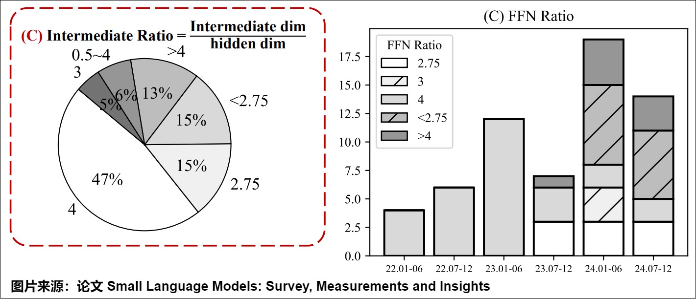
Implementations then round this theoretical width to an alignment multiple. One common policy is

$$d_{ff,impl} =m\left\lceil \frac{\rho(8d_{model}/3)}{m} \right\rceil,$$

where $m$ is an alignment multiple and $\rho$ is an optional width multiplier. The checkpoint’s stored intermediate_size remains authoritative because different model families choose different $m$, $\rho$, and bias policies.

Worked modern-width example:

d_model = 4096

classic:
    d_ff = 16384
    weights = 2 * 4096 * 16384
            = 134,217,728
    projection MACs/token = 134,217,728

SwiGLU-style:
    d_ff = 11008
    weights = 3 * 4096 * 11008
            = 135,266,304
    projection MACs/token = 135,266,304

The two choices are close in matrix budget, but their intermediate state is not identical:

classic:
    one [B,S,16384] expanded branch

SwiGLU:
    gate [B,S,11008]
    up   [B,S,11008]
    gated product [B,S,11008]

A fused implementation may avoid storing every named intermediate, but the dependency graph still exists. M4.1 integrates these counts across layers and training state; M3.6 must retain the local derivation because it explains why intermediate_size and the number of projections are inseparable architecture choices.

Bias and projection-count ledger

Including biases makes the distinction explicit:

$$P_{classic} =d_{model}d_{ff}+d_{ff} +d_{ff}d_{model}+d_{model},$$ $$P_{gated} =2(d_{model}d_{ff}+d_{ff}) +d_{ff}d_{model}+d_{model}.$$

Many decoder MLPs disable these biases, while the original Transformer FFN enabled them. A conversion that silently creates or drops biases can load most tensor shapes correctly and still change the function.

Exact budget matching with bias policies

The 2/3 rule is exact only for the large bias-free projection terms. Let $h_c$ be the classic width and $h_g$ the gated width. Introduce binary bias flags:

b1: classic expansion bias
b2: classic contraction bias
bg: gated gate-projection bias
bu: gated up-projection bias
bo: gated down-projection bias

Then

$$P_c=2d h_c+b_1h_c+b_2d$$

and

$$P_g=3d h_g+(b_g+b_u)h_g+b_od.$$

Solving $P_g=P_c$ gives

$$h_g = \frac{2dh_c+b_1h_c+(b_2-b_o)d} {3d+b_g+b_u}.$$

If every projection has a bias, this reduces to

$$h_g=h_c\frac{2d+1}{3d+2},$$

which approaches but does not exactly equal $2h_c/3$. If both architectures are bias-free, the familiar factor is exact. Parameter matching also does not match activation-function work: SwiGLU adds SiLU and a Hadamard product, while ReLU has a cheaper pointwise path.

Rounding is an architecture decision, not bookkeeping

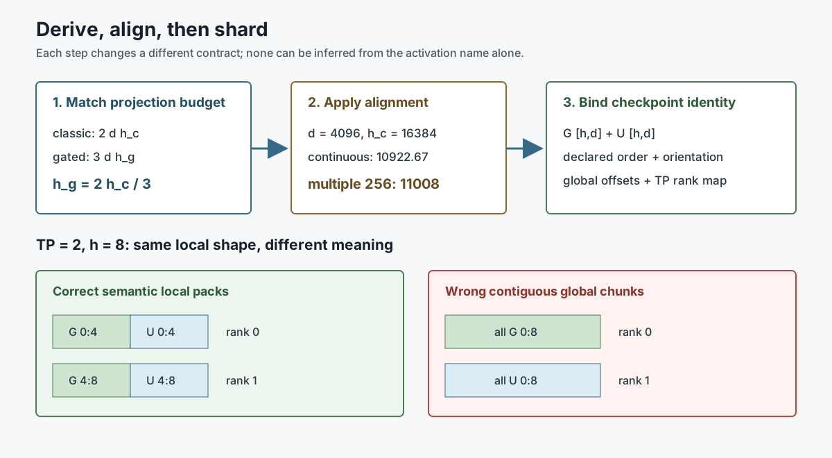
For a bias-free classic width $h_c=4d$, the continuous gated solution is $8d/3$. An implementation that rounds upward to multiple $m$ uses

$$h_{impl}=m\left\lceil\frac{8d}{3m}\right\rceil.$$

For d=4096 and m=256:

continuous width = 8 * 4096 / 3 = 10922.666...
aligned width    = ceil(10922.666... / 256) * 256
                 = 11008

The aligned SwiGLU layer has 1,048,576 more projection parameters than the unrounded equal-budget target:

$$3\cdot4096\cdot(11008-10922\tfrac23)=1{,}048{,}576.$$

It is still close to the classic d_ff=16384 budget, but “matched” should not be read as bit-exact equality after rounding. Rounding down changes the sign of the budget delta and may violate a kernel’s preferred tile multiple. The stored intermediate_size is part of the architecture and must not be recomputed by a loader.

Packed checkpoints and tensor-parallel resharding

Under PyTorch storage orientation, separate tensors have shapes:

G = gate_proj.weight: [h, d]
U = up_proj.weight:   [h, d]

A single-rank packed FC1 can store

$$W_{GU}=\begin{bmatrix}G\\U\end{bmatrix} \in\mathbb R^{2h\times d}$$

and split linear(x, W_GU) at h along the output axis. That is not enough to define a tensor-parallel checkpoint. With h=8 and TP=2, the semantic local packs are:

rank 0: [G[0:4]; U[0:4]]
rank 1: [G[4:8]; U[4:8]]

Naively cutting the global [G;U] tensor into two contiguous halves produces:

rank 0: [G[0:8]]
rank 1: [U[0:8]]

Both local arrays have shape [8,d], but neither rank can form a local gate/value product. This is the reason the pinned Megatron-Core path records a GLU stride and uses a sharded-tensor factory that splits the two logical halves before assigning global offsets.

A safe conversion is semantic, not byte-chunk based:

gate, up = unpack_source_by_declared_order(source_fc1)
assert gate.shape == up.shape == (h, d)

for rank in range(tp):
    g_local = gate[rank * h // tp : (rank + 1) * h // tp]
    u_local = up[rank * h // tp : (rank + 1) * h // tp]
    target_rank[rank] = cat([g_local, u_local], dim=0)

gate_roundtrip = cat([unpack_rank(r)[0] for r in ranks], dim=0)
up_roundtrip   = cat([unpack_rank(r)[1] for r in ranks], dim=0)
assert_equal(gate_roundtrip, gate)
assert_equal(up_roundtrip, up)

The conversion release gate must compare a known input through source and target layouts and perform this reshard round trip. Parameter counts alone cannot detect gate/up swaps, transposes, or incorrect TP offsets.

---

0x07 Forward and backward tensor mechanics

The forward graph is also the backward graph’s dependency map. For a classic row-major FFN, define

$$Z=XW_1+b_1,\qquad H=\phi(Z),\qquad Y=HW_2+b_2.$$

With flattened rows $T=B\cdot S$:

X:  [T, d_model]
W1: [d_model, d_ff]
Z:  [T, d_ff]
H:  [T, d_ff]
W2: [d_ff, d_model]
Y:  [T, d_model]

Let $G_Y=\partial\mathcal L/\partial Y$. Matrix calculus gives

$$G_{W_2}=H^\top G_Y, \qquad G_H=G_YW_2^\top,$$ $$G_Z=G_H\odot\phi'(Z), \qquad G_{W_1}=X^\top G_Z, \qquad G_X=G_ZW_1^\top.$$

Bias gradients reduce over the independent row axis:

$$G_{b_2}=\sum_{t=1}^{T}G_Y[t,:], \qquad G_{b_1}=\sum_{t=1}^{T}G_Z[t,:].$$

This derivation explains which forward objects autograd must retain or reconstruct. Computing $G_{W_2}$ needs $H$; computing $G_Z$ needs either $Z$ or enough activation state to recover $\phi'(Z)$; computing $G_{W_1}$ needs $X$.

SwiGLU backward path

For a bias-free gated MLP, define

$$G=XW_g,\qquad U=XW_u,\qquad H=\phi(G)\odot U,\qquad Y=HW_d.$$

The output projection backpropagates as before:

$$G_H=G_YW_d^\top, \qquad G_{W_d}=H^\top G_Y.$$

The Hadamard product splits the gradient into both input branches:

$$G_G=(G_H\odot U)\odot\phi'(G), \qquad G_U=G_H\odot\phi(G).$$

Both branches contribute to the input gradient:

$$G_X=G_GW_g^\top+G_UW_u^\top,$$

and their weight gradients are

$$G_{W_g}=X^\top G_G, \qquad G_{W_u}=X^\top G_U.$$

The two input matrices may have identical shapes, but their gradients are not interchangeable. Swapping gate and up weights changes where $\phi'$ appears.

Training-state trace

An unfused pedagogical implementation might expose:

def swiglu_train_trace(x, gate_w, up_w, down_w):
    gate_pre = x @ gate_w
    gate_act = silu(gate_pre)
    up = x @ up_w
    hidden = gate_act * up
    y = hidden @ down_w
    return y

During training, a framework may save x, gate_pre, gate_act, up, and hidden, or save fewer tensors and recompute some of them in backward. Activation checkpointing trades additional forward compute for lower retained activation memory; it does not change the mathematical graph.

Activation-memory ledger

Ignoring allocator padding and assuming a bytes per activation element:

classic named intermediates:
    Z + H ~= 2 * T * d_ff * a bytes

SwiGLU named intermediates:
    G + gate_act + U + H ~= 4 * T * d_ff * a bytes

This is an upper-level dependency ledger, not a promise that all four arrays are simultaneously resident. In-place activation, fused gate multiplication, saved-tensor policies, and recomputation can reduce materialized state. Conversely, backward workspaces and gradient buffers add state not shown here.

Saved-tensor schedules are implementation choices

The backward equations state dependencies, not one mandatory save policy. A training implementation can choose among at least three schedules:

Schedule	Retained local state	Backward action	Main tradeoff
eager/autograd-heavy	X, preactivations, activated branches, hidden product	reuse named tensors	largest retained activation set
fused custom backward	X, selected preactivation/branch state, compact mask/RNG metadata	kernel reconstructs cheap pointwise terms	less traffic, kernel-specific contract
activation checkpoint	boundary input plus RNG state	rerun input projections and gate before gradients	lower retained state, additional GEMMs

For SwiGLU, saving only $H=\operatorname{SiLU}(G)\odot U$ is insufficient: many $(G,U)$ pairs produce the same product, while the two backward branches need $U\operatorname{SiLU}'(G)$ and $\operatorname{SiLU}(G)$ separately. A valid custom backward must retain enough information or recompute both projections from $X$ and the current weights.

Checkpoint recomputation also has a temporal contract. If the forward includes dropout,

$$H_{drop}=\frac{M\odot H}{1-p}, \qquad M_j\sim\operatorname{Bernoulli}(1-p),$$

then backward uses

$$G_H=\frac{M\odot G_{H_{drop}}}{1-p}.$$

Recomputation must reproduce the same mask $M$, usually by preserving RNG state or a counter-based seed. Sampling a new mask does not reconstruct the forward graph. Deterministic replay also depends on the distributed RNG stream: two tensor-parallel ranks must not accidentally reuse a mask when the architecture expects distinct local-channel masks.

A concrete retained-activation ledger

Take pretraining rows T=8192, d_model=4096, BF16 activations, and the matched widths from the earlier example. One model-width tensor is

$$8192\cdot4096\cdot2\text{ bytes}=64\text{ MiB}.$$

One SwiGLU-width tensor is

$$8192\cdot11008\cdot2\text{ bytes}=172\text{ MiB},$$

while one classic-width tensor at d_ff=16384 is 256 MiB.

named dependency ledger, excluding output/workspaces:

classic:
    X                 64 MiB
    Z + H            512 MiB

SwiGLU:
    X                 64 MiB
    G + gate_act
      + U + H         688 MiB

This does not predict the allocator peak. A fused SwiGLU kernel may never materialize gate_act separately, and checkpointing may retain only X plus metadata. Conversely, autograd, gradient accumulation, communication buffers, and allocator fragmentation can increase the peak. The ledger’s purpose is to make every omitted or recomputed tensor explicit before M4 measures a runtime.

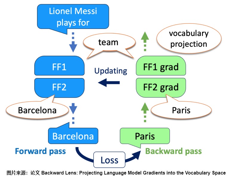
Weight gradients are minibatch sums of outer products

For any linear projection $Z=XW$ with flattened rows, the matrix gradient is

$$G_W=X^\top G_Z =\sum_{t=1}^{T}x_t^\top g_{z,t}.$$

A13 connects this outer-product structure to “imprint and shift” interpretations of how training changes MLP directions. The algebra is exact; the semantic interpretation is conditional. One optimizer step aggregates many token rows, loss terms, microbatches, and possibly data-parallel ranks, then transforms the gradient through clipping, weight decay, momentum, adaptive moments, and the learning-rate schedule. It is not generally a direct insertion of one prompt/target pair into one memory slot.

Local persistent training state

For an Adam-like optimizer, each trainable matrix can own:

checkpoint parameter
gradient or gradient shard
first moment
second moment
optional FP32 master parameter

The exact dtype and sharding of those objects are optimizer/runtime choices. They often dominate the persistent training memory far beyond the BF16 weight bytes, but M3.6 only inventories the state attached to its local matrices. M4.1 integrates it across layers and parallel groups.

The training manifest must therefore add:

initializer per projection
output-projection residual scaling, if any
hidden and wrapper dropout placements
activation-checkpoint boundary
RNG replay policy
gradient accumulation dtype
optimizer state dtype and sharding

Copying gate_proj, up_proj, and down_proj weights without those fields may reproduce inference while failing to reproduce continued training.

---

0x08 Runtime integration: eager graph, fusion, and sharding

The mathematical MLP can map to several execution plans.

Eager plan

GEMM gate/up
activation kernel
elementwise multiply
GEMM down

Each boundary can write and reread an intermediate from device memory. A fused SwiGLU kernel can combine the activation and Hadamard product, and implementations can concatenate gate and up weights:

$$W_{gu}=[W_g\;W_u], \qquad [G\;U]=XW_{gu}.$$

One larger GEMM then produces a tensor of shape [T, 2*d_ff], which is split logically before SiLU(G) * U. This fusion preserves the checkpoint function only if the packed weight order, split point, activation, bias, and dtype are correct.

def fused_input_projection(x, packed_w, d_ff):
    gu = x @ packed_w                 # [T, 2*d_ff]
    gate_pre, up = gu.split(d_ff, dim=-1)
    hidden = silu(gate_pre.float()).to(up.dtype) * up
    return hidden

The explicit .float() is one possible numerical policy, not a universal requirement. Production kernels may evaluate the activation in BF16, FP16, or an internal higher precision. Reproduction requires checking the specific kernel path.

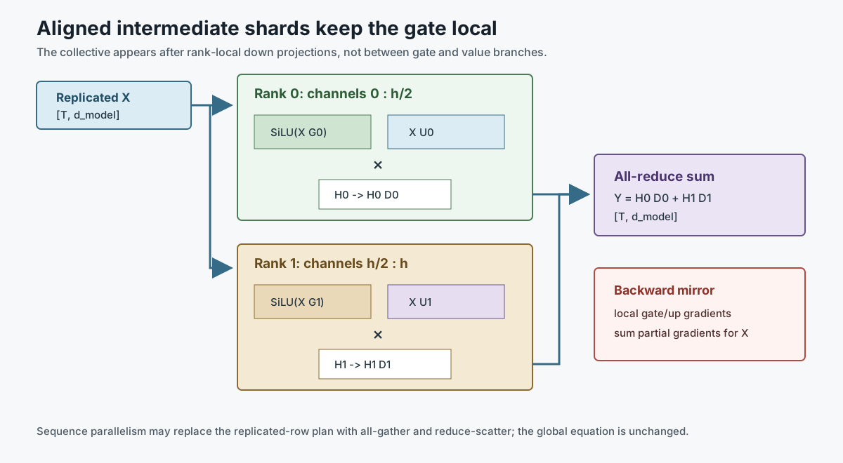
Tensor-parallel plan

A common Megatron-style decomposition shards the first projection by output features and the second by input features:

column-parallel gate/up:
    each rank owns a slice of d_ff
    local hidden: [T, d_ff / TP]

row-parallel down:
    each rank multiplies its local hidden slice
    partial outputs: [T, d_model]
    all-reduce sums partial outputs

For SwiGLU, the gate and up projections must use the same intermediate partition so their local elementwise product is defined. A mismatched sharding map can force communication before the gate or silently multiply unrelated channel slices.

Collective placement follows the algebra

Let tensor-parallel degree be $p$ and assume $d_{ff}$ is divisible by $p$. Partition the input projections by their output channels:

$$W_g=[W_g^{(0)}\;\cdots\;W_g^{(p-1)}], \qquad W_u=[W_u^{(0)}\;\cdots\;W_u^{(p-1)}].$$

Each rank receives the model-width row $X$ and computes

$$H^{(r)} = \operatorname{SiLU}(XW_g^{(r)})\odot XW_u^{(r)} \in\mathbb R^{T\times d_{ff}/p}.$$

Partition the down projection by matching input rows, $W_d=[W_d^{(0)};\ldots;W_d^{(p-1)}]$. Then

$$Y=\sum_{r=0}^{p-1}H^{(r)}W_d^{(r)}.$$

The local gate needs no collective because both branches share the same intermediate slice. The rank-local down projections produce model-width partials, so their sum is the first unavoidable forward collective in the classic Megatron layout.

Backward mirrors the ownership:

forward:
    replicated X
      -> local column-parallel gate/up
      -> local gated product
      -> local row-parallel down partial
      -> all-reduce partial Y

backward:
    output gradient
      -> local down/input-branch gradients
      -> local gate/up weight gradients
      -> all-reduce partial gradient for X

Exact libraries can overlap, fuse, or replace these collectives. With sequence parallelism, rows may be sharded between sublayers; an all-gather supplies rows before a column-parallel projection and a reduce-scatter returns row shards after the row-parallel projection. That changes tensor residency and collective type, not the global SwiGLU equation. M4 owns communication-byte and overlap performance; M3.6 owns the local tensor identities at each slot.

Pinned Megatron-Core source trace

At commit 23b2ff22, Megatron-Core’s MLP makes several contracts explicit:

if gated_linear_unit:
    fc1 output width is doubled
    stride = 2 records gate/linear grouping for resharding

linear_fc1:
    gather_output = False
    returns rank-local intermediate channels

activation:
    chunks the last axis into x_glu and x_linear
    computes activation(x_glu) * (x_linear + optional offset)

linear_fc2:
    input_is_parallel = True
    consumes the rank-local gated slice

The same source offers separate fused paths for bias-GELU, bias-GEGLU, and bias-SwiGLU. It can also clamp gate and linear branches or add a configured glu_linear_offset. Those are function-changing fields, not harmless kernel details. A checkpoint trained with a nonzero offset or clamp requires the same runtime semantics.

The module returns an output and possibly a deferred output bias. A surrounding bias/dropout/residual fusion may consume that bias, but M3.7 owns that wrapper. M3.6 records only that skip_bias_add=True changes where the MLP bias is materialized, not whether the learned affine term exists.

Four fusion levels must remain distinguishable

Fusion	Operators combined	Semantic fields that can break equivalence
input packing	gate GEMM + up GEMM as one [2h] GEMM	pack order, split axis, biases, TP offsets
pointwise gate	bias + activation + Hadamard product	activation variant, precision, clamp, offset
full MLP	FC1 + gate + FC2 in one runtime object	all prior fields plus accumulation and saved-tensor policy
block epilogue	output bias + dropout + residual add	dropout RNG, residual branch, M3.7 block order

Calling every row “fused SwiGLU” hides different blast radii. The release should name the fusion level and compare it against the same eager manifest.

Runtime conformance matrix

Before an optimized MLP is admitted, compare:

topology:
    classic, GEGLU, SwiGLU

layout:
    separate, packed, TP=1, TP>1, resharded checkpoint

mode:
    inference forward
    training forward + input and weight gradients
    activation checkpoint recomputation

numerics:
    supported parameter/input dtypes
    declared activation and accumulation policy

shapes:
    prefill-like many rows
    decode-like few rows
    non-contiguous input
    alignment boundary and odd row counts

Pass criteria must be tied to dtype and accumulation policy. The accompanying oracle proves the exact algebraic invariant in FP64-like Python arithmetic: a global SwiGLU output equals the sum of correctly aligned TP local down projections, and a packed gate/up projection equals the separate path.

Training versus inference

Concern	Training	Inference
dropout inside classic FFN	active according to architecture	disabled
forward intermediates	retained or recomputed for backward	disposable after down projection
gradients/optimizer state	required	absent
sequence rows	all supervised rows usually evaluated	prefill all rows; decode often one row/request
kernel choice	backward support and determinism matter	latency, batching, and weight residency dominate
tensor parallel	forward plus gradient collectives	forward collectives only

The MLP does not own KV cache state, but decode repeatedly invokes it for each newly produced row. Attention becomes increasingly bandwidth-sensitive as cached context grows; the dense MLP remains a fixed set of large matrix multiplications per decoded token. M4 and M5 compare those phase-level bottlenecks.

Configuration-to-runtime audit

Before loading an optimized kernel, bind every semantic field to a tensor or operation:

Configuration field	Runtime consequence	Wrong-but-shape-valid failure
hidden_size	input and output width	wrong residual-stream contract
intermediate_size	branch width and shard layout	checkpoint truncation/padding or split error
hidden_act	gate or hidden activation	different function with same weights
mlp_bias	adds one or three bias tensors	silent missing/additional affine offsets
gate/up order	packed split semantics	activation applied to wrong branch
tensor-parallel degree	local intermediate width	incompatible shard ownership
dtype/quantization	GEMM and activation numerics	overflow, drift, unsupported fused path

An implementation-level conformance test should compare at least:

eager reference output
optimized output
input gradient
each projection-weight gradient (training kernel)
multiple dtypes and non-contiguous input layouts

Checking only the final forward value can miss a custom backward that swaps gate and up derivatives.

---

0x08A Initialization, dropout, and activation statistics

MLP depth is trainable only if forward activations and backward gradients remain controlled. Initialization, normalization, and residual scaling are coupled even though M3.7 owns the full block.

Variance propagation through one classic FFN

Assume zero-mean independent input coordinates with variance $v_x$, and weights with variance $\operatorname{Var}(W_{1,ij})=\sigma_1^2$. Then each preactivation is a sum of $d_{model}$ terms:

$$\operatorname{Var}(Z_j) \approx d_{model}\sigma_1^2v_x.$$

Choosing $\sigma_1^2\propto1/d_{model}$ keeps this variance order-one. After activation, write

$$v_h=\mathbb E[\phi(Z)^2]-\mathbb E[\phi(Z)]^2.$$

The down projection gives approximately

$$\operatorname{Var}(Y_k) \approx d_{ff}\sigma_2^2v_h.$$

Thus $\sigma_2^2\propto1/d_{ff}$ controls the return projection. Xavier/Glorot and Kaiming initializers instantiate related fan-in/fan-out arguments under different activation assumptions. A real Transformer may additionally scale residual-branch output weights by depth; copying an isolated MLP initializer without the block’s residual policy is incomplete.

Gated-product variance is not the classic variance

For $H=\phi(G)\odot U$,

$$\mathbb E[H_j^2] =\mathbb E[\phi(G_j)^2U_j^2].$$

If the branches were independent, this factorizes into

$$\mathbb E[H_j^2] \approx\mathbb E[\phi(G_j)^2]\mathbb E[U_j^2].$$

They share the same input $X$, however, so exact independence is not guaranteed. This is why gated architectures should inherit the model family’s tested initialization rather than blindly reusing a two-matrix FFN prescription.

Dropout has two distinct placements

The Harvard FFN applies dropout to the activated hidden state before $W_2$:

$$Y=(m\odot\phi(XW_1+b_1))W_2+b_2,$$

with inverted-dropout mask

$$m_j=\frac{z_j}{1-p},\qquad z_j\sim\operatorname{Bernoulli}(1-p).$$

The wrapper can also apply dropout after the MLP output before residual addition. These are different random variables at different widths:

hidden dropout: [B,S,d_ff]
residual-branch dropout: [B,S,d_model]

Removing, moving, or sharing their masks changes training. Decoder-only LLM families often set these probabilities to zero at large scale, but that is an architecture choice rather than a universal MLP rule.

Activation sparsity and sparse-kernel reality

ReLU produces exact zero intermediates; GELU and SiLU generally produce small nonzero negatives. Thresholded or shifted activations can increase exact sparsity. A13 points to dReLU/TurboSparse as one such line of work.

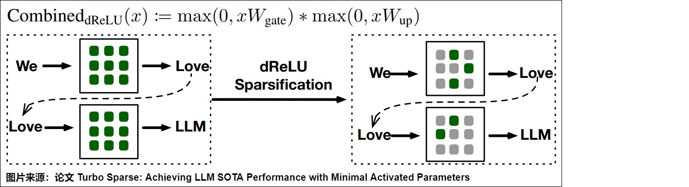
Algorithmic sparsity does not automatically become wall-clock speedup:

needed for useful sparse execution:
    enough zeros at the granularity supported by the kernel
    low-cost index/metadata generation
    hardware and library support
    load balance across rows and devices
    accuracy preserved under the trained sparse activation

A dense GEMM can outperform an irregular sparse path even when many mathematical values are zero. M4 owns the measured hardware conclusion; M3.6 records the activation property and the implementation condition.

---

0x09 What capacity means here

The dense MLP applies the same learned parameters to every token row:

for every row x[b, i, :]:
    y[b, i, :] = MLP(x[b, i, :])

Increasing d_ff increases the number of intermediate channels available to this per-row transformation. It also increases the projection weights and intermediate activation width.

This gives a narrow, implementation-facing meaning of MLP capacity:

more learned channel transformations available per token row

It does not mean the MLP is the only place where a model stores behavior or knowledge. Attention projections, embeddings, normalization parameters, and all other layers also participate in the learned function.

Feature-basis and key-value-memory interpretations

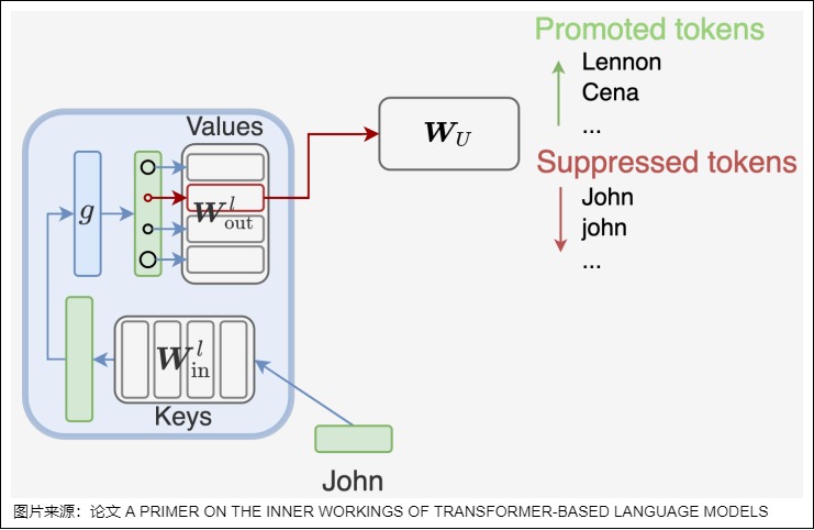
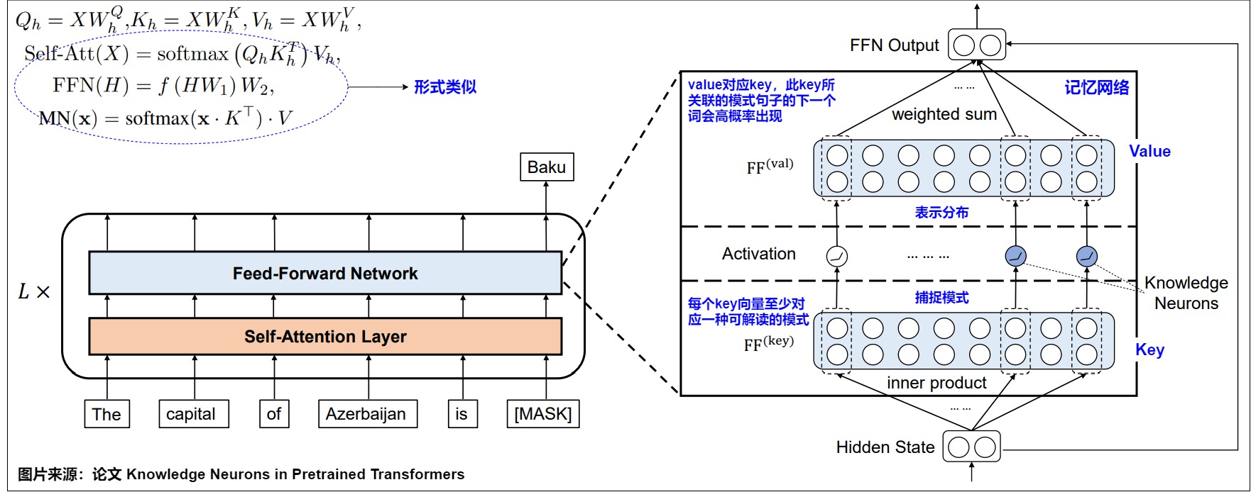
The paper Transformer Feed-Forward Layers Are Key-Value Memories analyzes FFN rows as learned pattern detectors and output directions. That can be a useful interpretive lens:

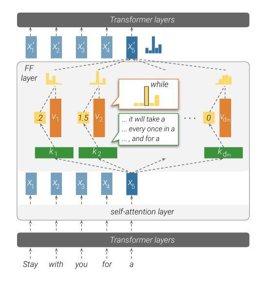
Source: Transformer Feed-Forward Layers Are Key-Value Memories, Figure 1. The diagram is an analysis of learned FFN behavior in the paper’s language-model experiments. It is not a separate runtime memory table and should not be confused with attention K/V tensors or the autoregressive KV cache.

first projection:
    detects learned input patterns

activation:
    controls which intermediate channels respond

second projection:
    maps active channels back into residual-stream directions

This is an interpretation of the learned computation, not a literal external key-value store, not an attention softmax, and not proof that all factual knowledge resides in the FFN.

The interpretation comes directly from expanding one row of a two-matrix FFN. Let the columns of $W_1$ be $k_i$ and the rows of $W_2$ be $v_i^\top$. Then

$$\operatorname{FFN}(x) =\phi(xW_1)W_2 =\sum_{i=1}^{d_{ff}}\phi(x^\top k_i)v_i^\top.$$

Each scalar $\phi(x^\top k_i)$ measures how strongly the current row matches an input direction $k_i$; the corresponding output direction $v_i$ is added with that coefficient. This looks like a set of key-triggered value directions, but it differs from attention in several ways:

FFN coefficients:
    produced independently per intermediate channel
    not normalized to sum to one
    can be negative for GELU/SiLU families
    use fixed learned directions at every token position

attention coefficients:
    compare query rows with sequence-dependent key rows
    are usually normalized across visible positions
    mix sequence-dependent value rows

The experiment contract behind “key-value memories”

The Geva et al. paper did not establish a universal ontology for every Transformer MLP. Its key-pattern experiment used:

model:
    fairseq transformer_lm.wiki103.adaptive
    247M parameters
    16 layers
    d_model = 1024
    d_ff = 4096

data:
    WikiText-103 training set

sample:
    10 keys per layer
    160 keys total out of 65,536 layer/key positions

trigger collection:
    rank all training-prefix representations by ReLU(x dot k_i)
    inspect the top 25 prefixes per sampled key

annotation:
    human experts identify repeated patterns appearing in at least 3 prefixes
    labels distinguish shallow and semantic patterns

The study reported at least one recognizable pattern for each sampled key and a shift from more shallow patterns in lower layers toward more semantic patterns in upper layers. Its value analysis projected value directions toward the vocabulary and compared them with tokens following the triggering patterns. The reported alignment was stronger in upper layers. Those are paper-specific correlations and annotations, not proof that every key has one stable meaning or that an individual value is a calibrated next-token distribution.

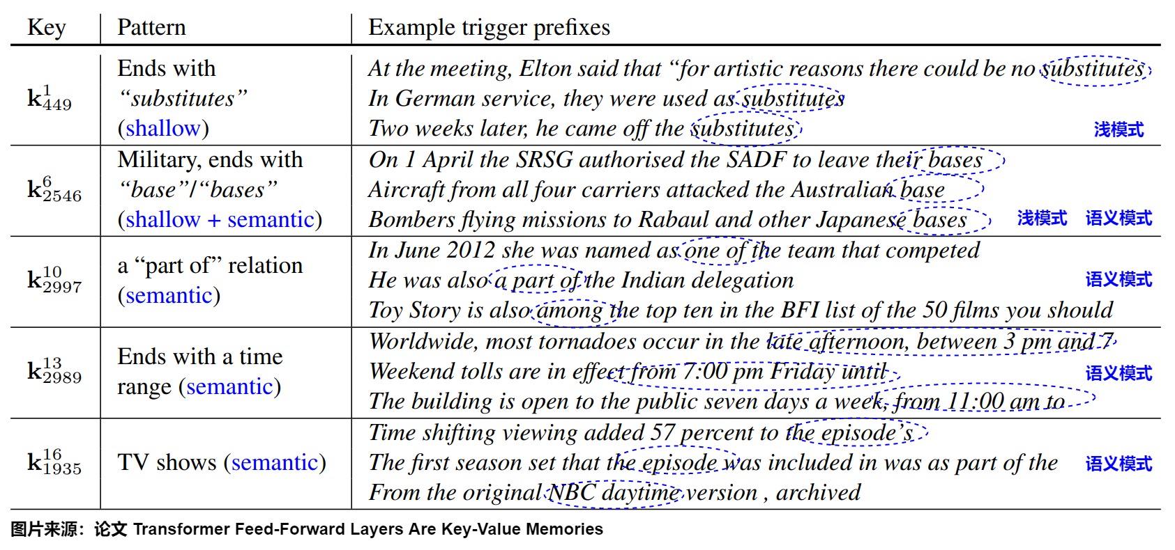
The paper itself notes an important difference from a normalized neural memory: its ReLU coefficients are unnormalized. In a modern GELU or SwiGLU model the coefficients can also be signed, weakening any interpretation as retrieval probabilities.

Gated MLPs require paired input directions

The basis-sum view still applies to a SwiGLU output, but the coefficient has a different form. Let $g_i$ and $u_i$ be column $i$ of gate and up matrices, and let $v_i^\top$ be row $i$ of the down matrix. Then

$$\operatorname{SwiGLU}(x) = \sum_{i=1}^{d_{ff}} \underbrace{ \operatorname{SiLU}(x^\top g_i)(x^\top u_i) }_{c_i(x)}v_i^\top.$$

Each output direction still has an input-dependent coefficient, but one intermediate channel now depends on a pair of learned input directions. Calling $g_i$ alone “the key” discards the linear branch $u_i$ that can amplify, suppress, or change the sign of $c_i(x)$. The gated analogy is therefore closer to a multiplicative feature interaction than a one-key lookup.

This distinction also changes intervention design:

intervene on gate preactivation:
    changes SiLU response and its derivative

intervene on up branch:
    changes the linear factor in the coefficient

intervene on gated product:
    bypasses both branch-generation mechanisms

edit down row:
    changes the residual direction contributed whenever that channel responds

Results from a two-matrix ReLU FFN cannot be transferred to those four objects without re-running the experiment on the gated checkpoint.

An evidence ladder for memory and feature claims

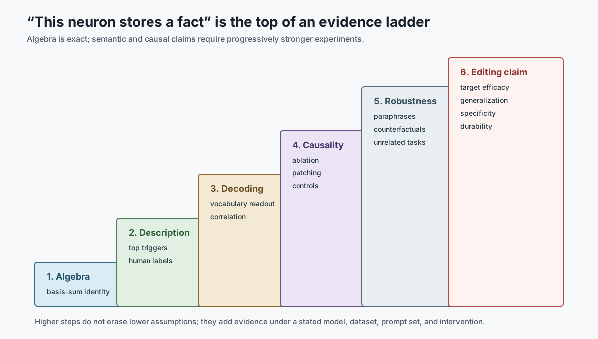
Level	Question	Evidence it supports	What it does not establish
algebra	can the output be written as coefficient-weighted directions?	exact basis/memory-like decomposition	semantic meaning
description	which inputs maximize one activation?	correlated trigger patterns	necessity or sufficiency
decoding	which vocabulary directions align with a value or activation?	readout association under a chosen decoder	causal use by the model
causal intervention	does ablation/patching change target behavior?	component contribution in tested contexts	unique storage location
behavioral robustness	does the effect survive paraphrases, controls, and counterfactuals?	broader functional role	harmless editability
editing	can a parameter change alter the target while preserving controls?	intervention efficacy and measured specificity	universal locality

A high activation is therefore a hypothesis generator. A defensible causal test needs matched controls, multiple phrasings, intervention baselines, and both necessity-like ablation and sufficiency-like activation/patching where possible. For factual knowledge, evaluate at least:

efficacy:
    target prompt changes as intended

generalization:
    paraphrases and related prompts change consistently

specificity:
    neighboring facts and unrelated capabilities remain stable

causal mediation:
    the proposed component carries measurable effect under patching/ablation

durability:
    effect survives generation contexts and later adaptation, if claimed

Knowledge use spans attention and MLPs

Handwritten A13 preserves a useful warning against reducing factual recall to one matrix. Mechanistic studies often decompose a recall path into subject enrichment, relation propagation, and output-attribute extraction across multiple attention and MLP sublayers.

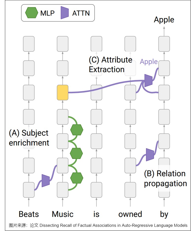
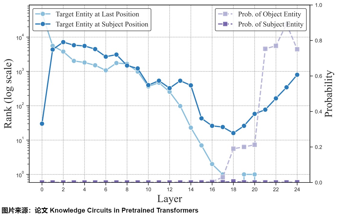
The figure is a causal analysis from a particular model and task, not a universal circuit diagram. The defensible conclusion is narrower:

some FFN channels correlate with reusable features or facts;
attention can move and combine those representations;
later layers can transform them into output-token evidence;
no single layer type owns all stored knowledge.

Localization, editing, and superposition

Knowledge localization asks which activations or parameters causally affect a behavior. Common tools include activation patching, causal tracing, gradients, integrated gradients, and direct/indirect effect measurements. Correlation alone is insufficient: a high activation can be a downstream readout rather than the cause.

Sparse autoencoders introduce an overcomplete dictionary $D$ and sparse code $s$ for an activation $h$:

$$s=\operatorname{TopK}\!\left(\phi(W_{enc}h+b_{enc})\right), \qquad \hat h=Ds+b_{dec}.$$

A typical training objective balances reconstruction and sparsity:

$$\mathcal L_{SAE} =\|h-\hat h\|_2^2+\lambda\|s\|_1,$$

or enforces an exact top-$k$ code instead of an $L_1$ penalty. The goal is to resolve superposed directions into a larger set of more interpretable features.

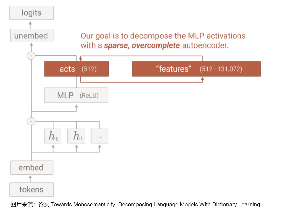
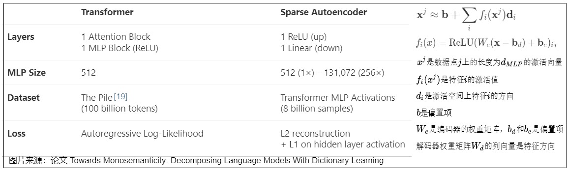
That decomposition is itself learned and lossy. A feature label is an interpretation, not a guaranteed ontology; dead features, feature splitting, reconstruction error, and cross-context polysemy remain audit concerns.

An SAE result should report at least reconstruction error, explained variance, sparsity or active-feature count, dead features, dictionary size, training data, and the effect of replacing the original activation with its reconstruction. Feature descriptions without that fidelity contract can mistake artifacts of the analysis model for properties of the Transformer.

Editing methods that alter an FFN matrix can change a target association, but locality is not guaranteed. A rank-one update $\Delta W=uv^\top$ changes every input with nonzero projection onto $u$:

$$(x(W+uv^\top))-xW=(xu)v^\top.$$

This equation explains both the attraction and the risk of low-rank edits: the update has a concise geometric target, yet any input aligned with $u$ receives the same output direction. Edit success therefore needs efficacy, paraphrase generalization, neighborhood specificity, and unrelated-capability regression tests.

---

0x0A Alternatives and design choices beyond a dense MLP

A dense MLP is one way to allocate nonlinear per-token capacity, not the only one. Alternatives are easiest to compare by asking which object they change:

activation-sparse dense MLP:
    keep dense matrices; make more intermediate coefficients exactly zero

Mixture of Experts:
    keep expert-shaped MLPs; route each token to a selected subset

trainable memory layer:
    replace selected dense FFNs with sparse learned key/value lookup

MemoryFormer:
    replace linear projections throughout a Transformer with learned hash tables

KAN:
    replace scalar edge weights plus node activations with learned edge functions

These are not interchangeable optimization flags. They imply different checkpoints, gradients, communication, kernels, and evidence requirements.

Activation-sparse dense MLPs: zeros are not yet speed

ReLU can create exact zeros, but a gated MLP remains nonzero when its two branches multiply to a nonzero value. Turbo Sparse’s dReLU changes both branches:

$$g(x)=\operatorname{ReLU}(xW_g), \qquad u(x)=\operatorname{ReLU}(xW_u),$$ $$h_{\mathrm{dReLU}}(x)=g(x)\odot u(x), \qquad y=h_{\mathrm{dReLU}}(x)W_d.$$

If the two branch preactivations were independent and symmetric around zero, a coordinate would be nonzero only when both were positive:

$$\Pr[h_i\ne 0] = \Pr[g_i>0]\Pr[u_i>0] =\frac14.$$

That toy calculation predicts $75\%$ zeros, not a universal sparsity level. Correlation, biases, normalization, training data, and learned weight geometry change the result. Turbo Sparse reports close to $90\%$ sparsity for its trained models, but that is a source-reported model result, not a property of the formula.

The paper contains two different contracts that must not be collapsed:

Contract	Starting point	Training	What the result establishes
controlled activation comparison	300M decoder-only models, dReLU versus SwiGLU	train both from scratch on 5B FineWeb tokens	paper-specific convergence and WikiText-2 comparison
ReLUfication pipeline	Mistral-7B and Mixtral-47B checkpoints	replace SwiGLU, continue pretraining on a stated data mixture, then SFT	recovery is a conversion-and-training pipeline, not a drop-in activation swap

For the conversion experiments, the paper reports up to 150B continued-pretraining tokens, AdamW, cosine scheduling, FSDP, and a web/code/math/academic/book mixture. Those details are part of the result. Removing them leaves no warrant for expecting the same quality after changing the activation.

Exact zeros also do not remove dense GEMM work automatically:

dense execution:
    compute every gate/up coordinate -> discover zeros -> dense down projection

sparse execution:
    identify active coordinates -> gather matching W_down rows
    -> sparse/dynamic matmul -> scatter/accumulate

The second path needs an activation predictor or a sparse representation, an efficient gather schedule, sparse kernels, and enough sparsity to repay indexing and load-imbalance overhead. Turbo Sparse’s reported decoding speedups use PowerInfer/PowerInfer-2 integration and particular hardware. They are source-reported system results, not FLOP-only consequences of dReLU.

Mixture of Experts

MoE keeps an expert-shaped MLP but routes each token to a subset of experts. It changes parameter activation, dispatch, balance, and communication rather than merely changing $\phi$.

M6 owns this branch in depth.

Trainable memory layers: sparse parameter lookup

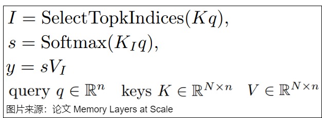
Memory Layers at Scale replaces selected dense FFNs with a learned table. Given query $q\in\mathbb{R}^{n}$, keys $K\in\mathbb{R}^{N\times n}$, and values $V\in\mathbb{R}^{N\times n}$, its basic sparse lookup is

$$I=\operatorname{TopKIndices}(Kq), \qquad s=\operatorname{softmax}(K_Iq), \qquad y=sV_I.$$

Here $I$ contains $k$ row indices, $K_I,V_I\in\mathbb{R}^{k\times n}$, and $s\in\mathbb{R}^{k}$. Each token performs this lookup independently. Unlike ordinary self-attention, $K$ and $V$ are persistent trainable parameters rather than sequence activations, and their row count can reach millions. Consequently both forward lookup and backward updates must be sparse.

Why product keys change the search cost

Scoring all $N$ trainable keys would destroy the intended compute advantage. The paper therefore uses product keys. For $N=M^2$ logical keys, store two half-key tables

$$K_1,K_2\in\mathbb{R}^{M\times n/2}, \qquad q=[q_1;q_2].$$

A logical key indexed by $(i,j)$ has score

$$\operatorname{score}(i,j) = K_{1,i}^{\top}q_1+K_{2,j}^{\top}q_2.$$

The full $M^2\times n$ key matrix is never materialized. The runtime first finds promising rows in each $M$-row half table and then ranks candidate pairs. With $M=1024$, the logical memory has $1{,}048{,}576$ keys while the first-stage search scores $2{,}048$ half keys per query, before candidate-pair ranking. This is a structured exact-search contract over the product key space, not an arbitrary ANN index that must be rebuilt after every key update.

Forward, backward, and persistent state

def memory_lookup(q, subkeys_1, subkeys_2, values, k):
    q1, q2 = split_last_dim(q)
    candidates_1 = topk(subkeys_1 @ q1, k)
    candidates_2 = topk(subkeys_2 @ q2, k)
    logical_ids, scores = topk_cartesian_sums(candidates_1, candidates_2, k)
    weights = softmax(scores, dim="selected_memory_rows")
    return weighted_embedding_bag(values, logical_ids, weights)

The saved state is not an FFN activation tensor alone:

State	Lifetime	Why it exists
subkey parameters and optimizer state	persistent training state	retrieval geometry is learned
value table and sparse optimizer state	persistent training state	selected rows store trainable output vectors
selected logical indices	forward-to-backward	backward must update the same rows
selected scores/softmax weights	forward-to-backward or recomputed	value and query gradients depend on them
duplicate-index map	backward kernel temporary state	several tokens may update one memory row

The paper reports custom EmbeddingBag kernels because duplicate sparse updates make backward accumulation nontrivial. It compares atomics, row locks, and a reverse-index schedule; that is a runtime contract, not an incidental implementation detail.

Parallel memory is not tensor parallelism

Memory values are sharded along their embedding dimension. Within a dedicated memory process group:

1. gather selected logical indices from all memory-group ranks;
2. each rank looks up and aggregates its local value-dimension shard;
3. exchange partial embeddings so each origin rank receives its token outputs;
4. preserve the sparse row ownership needed for backward updates.

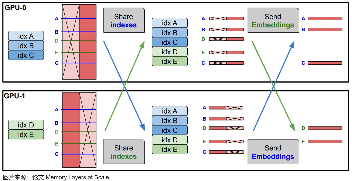
This collective is independent of the model’s tensor-, context-, or pipeline-parallel groups. A deployment manifest therefore needs a separate memory-group topology.

Shared memory and Memory+

The paper reuses one parameter pool from several layer positions. Sharing does not duplicate the table; it creates several query paths into the same parameters. In the reported ablation, three placements helped while replacing further FFNs degraded performance. That paper-specific result supports complementarity between sparse memory and dense computation, not replacement of every FFN.

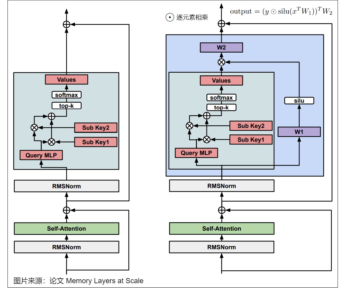
Memory+ wraps retrieved $y$ with an input-dependent gate:

$$\operatorname{MemoryPlus}(x) = \left(y\odot\operatorname{SiLU}(x^{\top}W_1)\right)^{\top}W_2.$$

The paper also uses query-key normalization when large memories become unstable. These additions demonstrate a design tension: sparse table capacity may be cheap in FLOPs, but stable conditioning and a useful nonlinear compute path can still require dense projections.

The authors explicitly note that production efficiency still requires substantial engineering. Dense GEMMs have decades of hardware/software co-design; a low-FLOP sparse lookup can remain bandwidth-, synchronization-, or kernel-bound.

MemoryFormer: hash-table approximation of linear maps

MemoryFormer is a different paper and a different memory contract. It trains a Transformer from scratch after replacing linear projections with groups of learnable hash tables. It replaces not only the FFN’s two projections but also the attention $Q/K/V$ projections; the classifier head remains fully connected in the reported models.

For a linear map $y=xW$, split $x\in\mathbb{R}^{d}$ into $K$ disjoint chunks $z_k\in\mathbb{R}^{\tau}$, where $d=K\tau$. Each chunk selects one of $2^{\tau}$ rows in table $T_k\in\mathbb{R}^{2^{\tau}\times h}$ from its sign bits:

$$h(z_k)=\operatorname{integer}(\operatorname{sign}(z_k)), \qquad \widehat y=\sum_{k=1}^{K}[T_k]_{h(z_k)}.$$

One table over all $d$ sign bits would require $2^d$ rows. Chunking changes the storage to

$$P_{\text{table}}=K\,2^{\tau}h.$$

For the paper’s example $d=h=512$, $\tau=8$, $K=64$, and FP16 values:

$$64\times 2^8\times512\times2\ \text{bytes} =16\ \text{MiB}.$$

The hard sign/index path is non-differentiable with respect to $z_k$. MemoryFormer therefore weights each selected row with a differentiable confidence

$$p(z_k) = \prod_{i=1}^{\tau} \frac{1}{1+\exp(-2|z_{k,i}|/t)},$$

and computes

$$\widehat y = \sum_{k=1}^{K}p(z_k)[T_k]_{h(z_k)}.$$

Gradients update selected table rows and flow to the input through $p(z_k)$, while no gradient passes through the discrete address itself. This is closer to a piecewise table approximation than to the top-$k$ associative memory above.

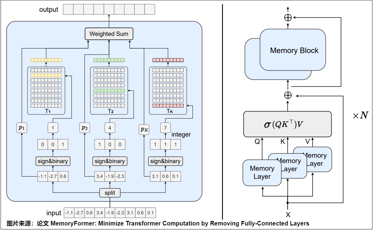
The reported Memory Block stacks two Memory Layers, normalizes before each lookup to keep sign buckets better occupied, omits an intermediate GELU because the hash is already nonlinear, and expands then contracts width through table shapes. Its Pythia-aligned experiments used Pythia-70M/160M/410M scales, the Pile, $\tau=8$, and a table learning rate three times the corresponding baseline because row gradients are sparse. Reported accuracy and FLOP numbers belong to that experiment contract.

It is therefore an alternative architecture, not a drop-in activation change and not a direct conversion of a standard dense checkpoint. Its sign buckets also create occupancy, discontinuity, table-capacity, and memory-bandwidth questions that a dense MLP does not have.

Kolmogorov-Arnold Networks

KANs move learnable nonlinear functions from nodes to edges. For input width $n_{\mathrm{in}}$ and output width $n_{\mathrm{out}}$, a layer is a matrix of functions:

$$y_j=\sum_i\phi_{j,i}(x_i),$$

where each edge function may contain a base function and a learned spline:

$$\phi_{j,i}(x) = w_b b(x) + w_s\sum_{r}c_rB_r(x).$$

A standard MLP instead learns scalar edge weights and applies a shared fixed activation at nodes. A KAN checkpoint must store basis coefficients and grid metadata for every edge; training may update spline grids as activation ranges move.

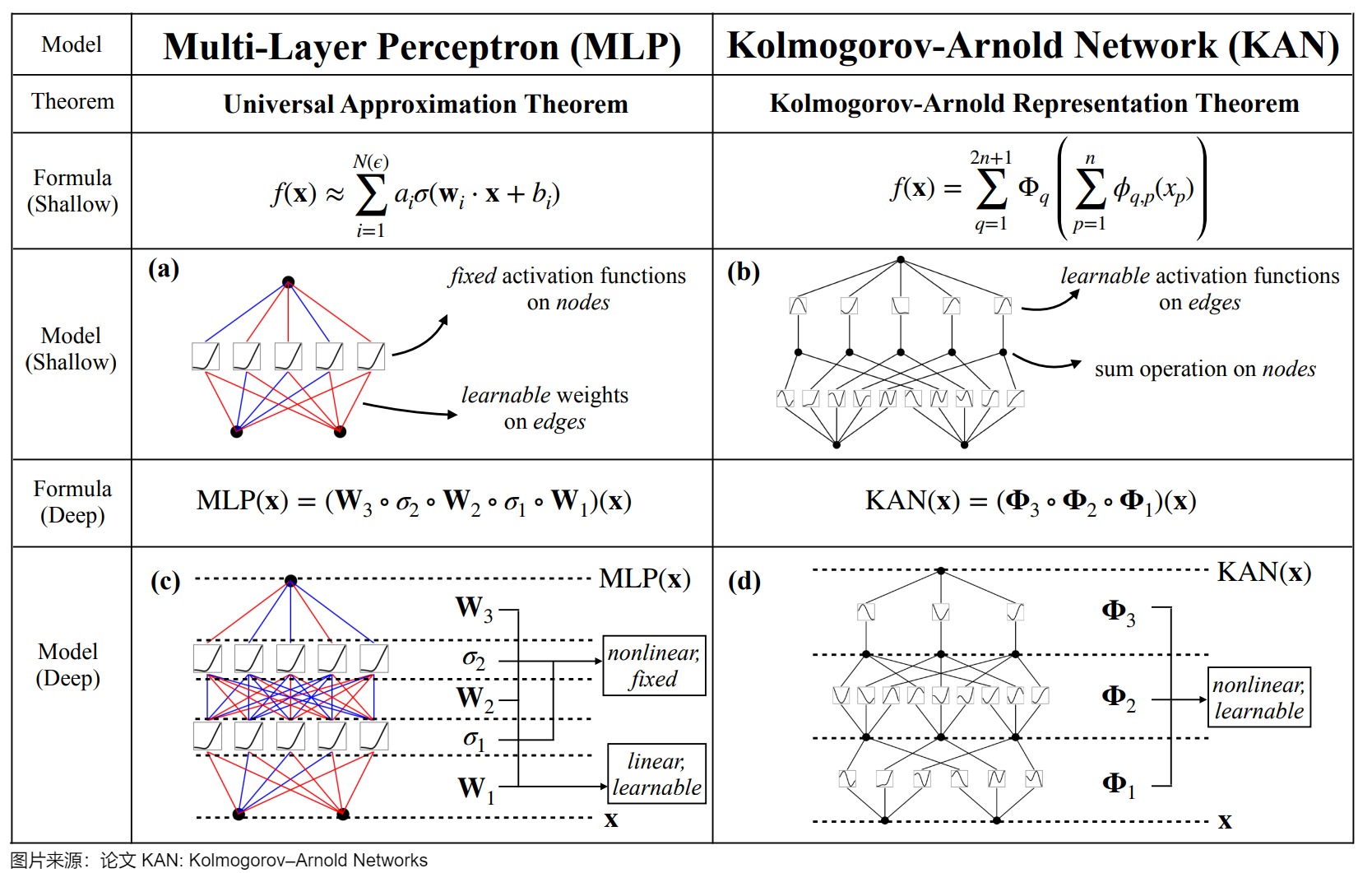
The original KAN paper’s strongest experiments are small-scale function fitting, PDE solving, and scientific interpretability. It explicitly reports its implementation as typically about $10\times$ slower to train than the compared MLP in the PDE experiment and leaves language modeling as future work. Its faster scaling-law results therefore cannot be transferred to production Transformer MLPs without new evidence. Edge-function evaluation, grid adaptation, parameter count, accelerator utilization, and language-model scaling all need measurement.

Paper-by-contract comparison

Method	Object changed	Checkpoint contract	Training contract	Runtime primitive	Evidence boundary
dReLU / Turbo Sparse	activation on both gated branches	activation swap requires recovery, unless trained from scratch	300M scratch comparison or continued pretraining + SFT for converted checkpoints	dense or sparse gated GEMM; sparse speed needs runtime support	reported sparsity/speed are model, data, engine, and hardware specific
MoE	token-to-expert parameter activation	router and expert tensors must exist	routing/balance/capacity objectives	dispatch, expert GEMM, combine, often all-to-all	owned by M6, not inferred from dense MLP behavior
Memory Layers at Scale	selected FFNs become sparse trainable associative tables	no lossless map from arbitrary FFN matrices	pretrain memory keys/values, sparse updates, stability controls	product-key search + weighted embedding bag + memory-group collectives	source-reported up to 128B memory parameters; production efficiency remains open
MemoryFormer	linear projections become sign-hash lookup tables	train-from-scratch architecture in the paper	sparse row updates, normalized hash inputs, higher table LR	address generation + table gather + weighted sum	experiments at Pythia-70M/160M/410M-aligned scales
KAN	scalar edges become learned univariate functions	new basis/grid tensors; no dense-checkpoint equivalence	backprop through basis coefficients plus grid adaptation	spline/basis evaluation and reduction	original evidence is mostly function fitting, PDEs, and scientific tasks

The decision is a systems decision

Before adopting any alternative, record at least:

architecture:
    changed operator, dimensions, persistent parameters, addressing/routing rule

training:
    from-scratch or conversion, data, optimizer, sparse-state ownership,
    stability controls, recovery budget

runtime:
    active rows/experts/edges, indexing cost, kernel, communication group,
    temporary buffers, backward accumulation

evaluation:
    matched parameter/compute baseline, quality tasks, throughput and latency,
    memory residency, hardware, batch and sequence regime

release:
    checkpoint compatibility, fallback implementation, rollback checkpoint,
    manifest and source revision

The right comparison is not “which formula looks cheaper?” It is which complete training-and-runtime contract improves the target workload without losing quality, reproducibility, or rollback.

---

0x0B Dense MLP boundary with MoE

In a dense FFN, every token uses the same MLP parameters:

all token rows -> one shared dense FFN

Mixture-of-Experts changes that capacity contract:

token rows -> router -> selected FFN experts -> combine

M3.6 establishes the dense expert-shaped unit and compares the alternative contract. M6.1 owns routing, expert selection, capacity limits, dispatch, combination, and total-versus-active parameter accounting.

The boundary matters because MoE usually changes the FFN side of the Transformer block, not the scaled dot-product attention equation.

---

0x0C Residual and normalization boundary

The MLP class returns a model-width update:

MLP(x): [B, S, d_model]

That shape allows a residual wrapper to combine the update with the residual stream. A common Pre-LN path is:

residual = x
u = norm(x)
u = mlp(u)
u = dropout(u)
y = residual + u

But those operations are not hidden inside the Harvard PositionwiseFeedForward class or the LLaMA LlamaMLP class.

M3.7 owns:

residual stream
normalization placement
dropout placement around sublayer output
Pre-LN versus Post-LN
attention + MLP block assembly

M3.6 owns only the per-row channel transformation that fits inside that wrapper.

---

0x0D What M3.6 does not own

Boundary	M3.6 imports	M3.6 does not re-teach
M3.2	attention returns [B,S,d_model] state rows	Q/K/V projections, head split, score path, W_O
M3.7	MLP input/output preserve residual-stream width	residual addition, LayerNorm/RMSNorm, Pre-LN/Post-LN, full block order
M4.1	local two- versus three-projection parameter/MAC ledger	layer/model totals, bytes, HBM traffic, kernel fusion
M6.1	dense FFN is the expert-shaped baseline	routers, top-k experts, dispatch, balancing, capacity overflow
M8.9	matrices and activations can become optimization targets	quantization, pruning, sparse kernels, deployment policy

M3.6 is a dense and gated MLP article. It treats knowledge analysis and alternatives deeply enough to preserve A13’s reasoning, but it is not a MoE implementation article, a model-editing recipe, or a whole-model cost model.

---

0x0E Shape ledger

Classic two-matrix FFN

Object	Shape	Notes
input x	[B,S,d_model]	contextual state rows
algebraic W_1	[d_model,d_ff]	row-vector notation
PyTorch w_1.weight	[d_ff,d_model]	stored Linear weight
w_1(x)	[B,S,d_ff]	expanded channels
activation	[B,S,d_ff]	ReLU/GELU/etc.
hidden dropout	[B,S,d_ff]	Harvard source placement
algebraic W_2	[d_ff,d_model]	contraction
PyTorch w_2.weight	[d_model,d_ff]	stored Linear weight
output	[B,S,d_model]	residual-compatible width

SwiGLU-style gated MLP

Object	Shape	Notes
input x	[B,S,d_model]	shared by both input branches
gate_proj(x)	[B,S,d_ff]	activated branch
SiLU(gate_proj(x))	[B,S,d_ff]	gate values
up_proj(x)	[B,S,d_ff]	linear branch
gated product	[B,S,d_ff]	elementwise multiply
down_proj(...)	[B,S,d_model]	returns to residual width

Axis ownership

Axis	FFN behavior
batch B	preserved, rows processed independently
sequence S	preserved, no direct cross-position mixing
channel d_model	transformed and expanded
intermediate d_ff	temporary nonlinear/gated capacity axis

---

0x0F Evaluation and validation contract

An MLP release is not validated by one successful forward pass. Validation has to close the algebra, checkpoint, training, distributed, runtime, and behavioral contracts exposed in this article.

Level 1: static architecture reconciliation

Before loading weights, derive the expected objects from the immutable manifest:

classic FFN:
    W_in [h,d], b_in [h], W_out [d,h], b_out [d]

separate SwiGLU:
    W_gate [h,d], W_up [h,d], W_down [d,h]

packed SwiGLU:
    W_gate_up [2h,d], split order declared, W_down [d,h]

Then reconcile:

1. expected parameter count against checkpoint tensor numel;
2. every tensor name, shape, dtype, bias policy, and alias;
3. continuous versus rounded intermediate width;
4. packed branch order and tensor-parallel partition metadata;
5. checkpoint format and source implementation revision.

No shape-compatible load should silently choose activation, approximation, branch order, or bias policy.

Level 2: local numerical and gradient oracles

Comparison	Required inputs	Acceptance signal	Failure localized
separate versus packed gated MLP	same weights, deterministic rows	elementwise forward and input/weight-gradient agreement	pack order or split axis
eager versus fused activation/gate	normal, large, near-zero, and non-finite probes by dtype	stated absolute/relative tolerance and matching non-finite policy	approximation or accumulation contract
unsharded versus tensor-parallel MLP	identical global tensors and rank-local shards	reconstructed forward and backward agreement	shard axis or collective slot
ordinary versus checkpointed training	same input, weights, and RNG seed	output/loss/gradient agreement	missing saved state or RNG replay
analytic versus finite-difference derivative	nonsingular scalar probes	bounded derivative error	activation or gated backward formula

Run these comparisons in the dtypes and backends that will ship. FP64 oracle agreement does not certify a BF16 fused kernel.

Level 3: training-state continuity

At initialization and after resume, record at least:

per layer and branch:
    input/output RMS
    gate and up preactivation mean/std/quantiles
    exact-zero fraction and thresholded-small fraction
    gate-up correlation
    saturation/non-finite counts
    parameter and gradient RMS
    optimizer step and loss-scale state

For dropout, compare an uninterrupted run with save/resume from the release checkpoint under the declared RNG restoration policy. For a conversion, compare loss before conversion, immediately after conversion, and through the recovery schedule; the immediate loss discontinuity is part of the artifact, not noise to hide.

Level 4: workload and systems evaluation

Measure the actual phase and shape regime:

Workload	Hold fixed	Report
training	tokens, optimizer, global batch, sequence distribution, hardware	tokens/s, step time, peak memory, communication, loss trajectory, downstream quality
prefill	prompt-length distribution, batch policy, output contract	TTFT, throughput, HBM traffic, temporary memory
decode	active batch, generation length, cache policy	inter-token latency percentiles, tokens/s, power, resident state
sparse activation	model quality and sparse-kernel engine	actual zero/active distribution by layer, predictor overhead, gather/scatter cost, achieved speedup
memory layer	table size, top-$k$, placement, memory group	lookup and backward time, duplicate-row skew, bandwidth, collective bytes, quality
architecture replacement	training tokens/compute and evaluation suite	matched baseline, quality, compute, resident memory, latency, failure rate

FLOPs, active parameter count, and wall-clock speed are three different ledgers. Report all three when the method changes sparsity or lookup.

Level 5: interpretation and intervention evaluation

Feature or memory claims require a separate protocol: held-out triggers, controls, activation statistics, causal ablation/patching, paraphrase generalization, neighborhood specificity, unrelated-task regression, and seed/model replication. A high decoding score or a successful edit is evidence under that protocol; it is not a substitute for runtime or language-model quality evaluation.

---

0x10 Failure lab

Axis and shape bugs

1. Applying the FFN across the sequence axis. The learned projections should transform the last feature axis. Mixing S changes the operation into token mixing.

2. Transposing to [B,d_model,S] before nn.Linear(d_model,d_ff). The final dimension no longer matches in_features.

3. Wrong contraction width. If the second projection does not return d_model, the later residual addition cannot preserve the stream shape.

4. Treating d_ff = 4d_model as a universal law. It is one architecture choice. The checkpoint configuration is authoritative.

5. Confusing algebraic and PyTorch weight orientation. A transpose mistake can break checkpoint conversion while all named dimensions look familiar.

Activation and dropout bugs

6. Activation after the second projection. That is not the classic Linear -> activation -> dropout -> Linear source path.

7. Removing the activation and assuming depth is preserved. Two affine maps without an intervening nonlinearity collapse into one affine map.

8. Loading a ReLU/GELU checkpoint under a SiLU configuration. Weight shapes can match while the model function changes.

9. Dropout placed in a different location from the trained architecture. Hidden dropout, sublayer-output dropout, and attention dropout are separate objects.

10. Dropout active during evaluation. The MLP output becomes stochastic when the inference contract expects evaluation mode.

SwiGLU bugs

11. Replacing ReLU with SiLU but keeping only two matrices. That creates a SiLU FFN, not a SwiGLU MLP.

12. Adding the gate and up branches instead of multiplying them. SwiGLU uses an elementwise product.

13. Applying a second sigmoid to up_proj(x). The verified LLaMA path multiplies SiLU(gate_proj(x)) by the linear up_proj(x) branch.

14. Gate/up intermediate widths disagree. Elementwise multiplication requires matching [B,S,d_ff] shapes.

15. Using the classic FFN d_ff without auditing the third projection. Parameter and compute assumptions change when the architecture adds another input matrix.

16. Swapping gate_proj and up_proj during checkpoint conversion. Shapes remain identical, but the activation is applied to the wrong learned branch.

17. Assuming all SwiGLU implementations use bias or all omit it. Bias is a configuration/checkpoint choice. The primary comparison omitted bias; Transformers v5.13.1 exposes mlp_bias.

Boundary bugs

18. Claiming the FFN mixes tokens. Attention or another sequence operator performs row mixing; the dense FFN acts on each row separately.

19. Placing residual addition inside the MLP implementation without matching the checkpoint architecture. The sublayer and its wrapper are separate contracts.

20. Treating the key-value-memory interpretation as literal storage. It is an analytical interpretation of learned projections and activations.

21. Treating one dense FFN as an MoE router. Conditional expert selection introduces different objects owned by M6.

22. Turning the local MLP ledger into a whole-model hardware claim. M3.6 counts its own matrices, MACs, and intermediate rows. M4.1 integrates them across layers and phases and analyzes bytes, HBM traffic, and hardware bottlenecks.

Training and runtime bugs

23. Saving only the gated product and assuming backward can recover both branches. In general, H = SiLU(G) * U does not uniquely determine G and U; backward must retain or recompute sufficient state.

24. Sharding gate and up projections differently. Local Hadamard multiplication requires aligned intermediate-channel partitions.

25. Packing [up, gate] weights but splitting the fused result as [gate, up]. The shape and allocation remain valid while the learned function changes.

26. Assuming a fused activation uses the same approximation and precision as eager mode. GELU approximation, SiLU precision, and accumulation dtype can create reproducibility differences.

27. Comparing a two-matrix FFN and a three-matrix GLU at the same d_ff and calling the parameter budget matched. Equal intermediate width gives the gated path roughly 50% more projection weights; derive and round the comparable width first.

Interpretation bugs

28. Treating FFN coefficients as an attention distribution. They are not normalized across channels and may be signed.

29. Calling one intermediate neuron a fact without causal and behavioral tests. Activation correlation does not establish storage, necessity, or sufficiency.

30. Assuming a low-rank edit is local because its rank is small. Every input with projection onto the update’s input direction is affected.

31. Treating sparse-autoencoder features as ground-truth concepts. Dictionary learning introduces reconstruction, sparsity, feature-splitting, and labeling assumptions.

Alternative-architecture bugs

32. Equating activation sparsity with sparse execution. A dense kernel still multiplies through coordinates that later become zero. Measure predictor, indexing, gather/scatter, and sparse-kernel overhead.

33. Replacing SwiGLU with dReLU and skipping recovery training. Turbo Sparse’s conversion result includes continued pretraining, a specified data mixture, and SFT. The activation swap alone is not the paper’s contract.

34. Searching every row of a million-entry memory table. Full key scoring defeats the sparse-compute objective. Product-key decomposition and candidate-pair ranking are part of the architecture.

35. Treating the memory process group as the MLP tensor-parallel group. Parallel memory exchanges selected indices and value-dimension shards under a separate ownership contract.

36. Calling MemoryFormer a converted dense checkpoint. The paper trains a replacement architecture from scratch and changes attention projections as well as FFNs.

37. Backpropagating through a hard sign address as if it were differentiable. MemoryFormer’s input gradient uses its continuous confidence factor; selected table rows receive sparse updates, while the discrete index has no derivative.

38. Transferring KAN scaling claims directly to language-model MLPs. The original evidence is primarily function fitting, PDE solving, and scientific tasks, and the paper leaves language modeling as future work.

39. Presenting a paper figure without its experiment boundary. A visual can preserve useful mechanism detail while still misleading if its model, task, source, or source-reported status is omitted.

Release and rollback bugs

40. Shipping a checkpoint without its architecture manifest. Width, activation, packing, biases, dtype, and sharding cannot be reconstructed safely from tensor shapes alone.

41. Promoting a fused kernel after testing only eager FP32. The shipped backend and dtype need their own numerical, non-finite, gradient, and performance checks.

42. Overwriting the last compatible checkpoint during conversion. Rollback requires immutable old weights, optimizer/RNG state when training resumes, runtime configuration, and a tested previous code path.

---

0x11 Release and rollback contract

A releasable MLP artifact is a bundle, not a weight file:

{
  "architecture": {
    "family": "swiglu",
    "d_model": 4096,
    "d_ff": 11008,
    "bias": false,
    "activation": "silu",
    "packing": "gate_then_up",
    "tensor_parallel_size": 8
  },
  "checkpoint": {
    "format": "declared-format",
    "sha256": "immutable-content-hash",
    "source_revision": "training-code-revision"
  },
  "runtime": {
    "backend": "declared-backend",
    "kernel_id": "declared-kernel-and-version",
    "parameter_dtype": "bf16",
    "activation_dtype": "bf16",
    "accumulation_dtype": "fp32"
  },
  "validation": {
    "oracle_report": "content-addressed-report",
    "distributed_report": "content-addressed-report",
    "quality_report": "content-addressed-report",
    "workload_report": "content-addressed-report"
  },
  "rollback": {
    "checkpoint_sha256": "previous-compatible-checkpoint",
    "runtime_manifest": "previous-runtime-manifest",
    "procedure_tested": true
  }
}

For a from-scratch alternative such as MemoryFormer, the rollback target is the previous architecture release, not an attempt to reinterpret hash tables as dense matrices. For a converted activation, retain the pre-conversion checkpoint and optimizer/RNG state until the recovery and regression gates pass. For a kernel-only change, retain an eager or previously approved implementation under the same checkpoint contract.

Promotion gates

gate 1: manifest and checkpoint reconcile exactly
gate 2: local forward/backward and dtype oracles pass
gate 3: distributed reconstruction and checkpoint reshard pass
gate 4: resume/recovery training state is continuous or explained
gate 5: target quality and regressions meet declared thresholds
gate 6: target workload improves under the deployed engine
gate 7: rollback is rehearsed from the release bundle

If a gate fails, keep the evidence and reject the release. Do not weaken the manifest after seeing the result.

---

0x12 Handoff

M3.1 and M3.2 built the sequence-mixing sublayer:

[B,S,d_model]
    -> multi-head attention
    -> [B,S,d_model]

M3.6 has now built the channel-mixing sublayer:

[B,S,d_model]
    -> dense or gated per-token MLP
    -> [B,S,d_model]

M3.7 can assemble both around one residual stream:

X_l
    -> norm / attention / dropout / residual
    -> norm / MLP / dropout / residual
    -> X_{l+1}

The full block preserves the state-row contract while alternating two kinds of work:

attention:
    route information across rows

MLP:
    transform channels inside each row

That is the handoff from sublayer mechanics to Transformer block assembly.

---

0xFF References

• Exploring the Transformer Series (13) — FFN
• M3.2 — Multi-Head Attention Layout
• M3.7 — Residual Stream and Block Assembly
• M4.1 — Transformer Cost Model
• M6.1 — Routed Capacity: MoE Experts, Routers, and Token Dispatch
• Vaswani et al., Attention Is All You Need
• Dauphin et al., Language Modeling with Gated Convolutional Networks
• Hendrycks and Gimpel, Gaussian Error Linear Units (GELUs)
• Ramachandran et al., Searching for Activation Functions
• Shazeer, GLU Variants Improve Transformer
• Raffel et al., Exploring the Limits of Transfer Learning with a Unified Text-to-Text Transformer
• Chowdhery et al., PaLM: Scaling Language Modeling with Pathways
• Touvron et al., LLaMA: Open and Efficient Foundation Language Models
• Shoeybi et al., Megatron-LM: Training Multi-Billion Parameter Language Models Using Model Parallelism
• Sukhbaatar et al., End-To-End Memory Networks
• Geva et al., Transformer Feed-Forward Layers Are Key-Value Memories
• Geva et al., Dissecting Recall of Factual Associations in Auto-Regressive Language Models
• Yao et al., Knowledge Circuits in Pretrained Transformers
• Dai et al., Knowledge Neurons in Pretrained Transformers
• Meng et al., Locating and Editing Factual Associations in GPT
• Bricken et al., Towards Monosemanticity: Decomposing Language Models With Dictionary Learning
• Song et al., Turbo Sparse: Achieving LLM SOTA Performance with Minimal Activated Parameters
• Lample et al., Large Memory Layers with Product Keys
• Lample et al., Memory Layers at Scale
• Xu et al., MemoryFormer: Minimize Transformer Computation by Removing Fully-Connected Layers
• Liu et al., KAN: Kolmogorov-Arnold Networks
• Hugging Face Transformers v5.13.1, LlamaMLP in modeling_llama.py
• Hugging Face Transformers v5.13.1, LlamaConfig
• NVIDIA Megatron-LM commit 23b2ff2, megatron/core/transformer/mlp.py