M6.11 - Pruning, Structural Compression, and Executable Sparsity

0x00 Removing Parameters Is Not Yet Acceleration

A large Transformer has already been trained. Its quality is useful, but its deployment graph is too expensive. We may want fewer stored bytes, a lower memory-bandwidth requirement, smaller matrix multiplications, fewer blocks, or a model that fits on fewer devices. This creates a question that sounds simple:

Which parts of the trained model can be removed without destroying the behavior that made the model useful?

The word pruning covers the family of methods that answer this question by removing parameter values or structural components. The idea predates Transformers: an overparameterized network may contain weights, neurons, or modules whose removal changes the useful function less than their resource cost would suggest. Transformers make the question more structured. Their weights are organized into attention heads, Q/K/V/O projections, MLP channels, residual-width channels, repeated blocks, embedding tables, and normalization state. A pruning decision can therefore range from one scalar entry to an entire layer.

The introductory distinction in Section 6.4.7 of the local book remains useful:

unstructured pruning
    -> remove individual connections or scalar weights

structured pruning
    -> remove complete groups such as heads, channels, or layers

But this distinction is not sufficient for implementation. A matrix containing millions of exact zeros can still occupy its original dense tensor, load every zero from memory, and execute the same dense GEMM. Conversely, deleting an MLP channel requires changing several coupled matrices, not placing one isolated zero in one tensor. A shorter layer list changes the ordered function graph and checkpoint configuration. Hardware-constrained 2:4 sparsity stores values plus compact pattern metadata and requires an eligible sparse operator.

The pruning problem is therefore not only what should become zero? It is:

what unit is removable?
what evidence says it is removable?
what budget and schedule create the mask or structure?
what artifact exists after transformation and recovery?
what runtime can execute that artifact more cheaply?

These questions form the spine of M6.11.

0x00A Pruning Changes A Different Object From Quantization Or Distillation

Pruning appears next to quantization and distillation in model-compression surveys, but their primary changed objects are different:

Method	Changed object	Typical training or calibration state	Runtime consequence
quantization	numerical alphabet and scale/metadata used to represent tensors	calibration and/or fake-quantized optimization	lower-bit storage and compatible low-bit kernels
distillation	student training objective and teacher-derived supervision	teacher logits, features, sequences, or cached targets	ordinary student runtime if teacher state is excluded
unstructured pruning	selected scalar weight entries	score, mask, optional reconstruction/retraining	no automatic saving unless sparse storage and kernels are used
N:M pruning	a locally constrained nonzero pattern	local group selection and optional recovery	hardware/library-specific semi-structured sparse path
structured width pruning	heads, MLP channels, residual channels, or coupled groups	importance/search, tensor surgery, recovery	physically smaller dense projections when dependencies close
depth pruning	complete blocks/layers	layer selection or training-time preparation, then recovery	fewer block invocations and a shorter graph

The methods can be composed. A pruned model can be quantized. A teacher can supervise recovery after structural removal. A quantization-aware student can also carry an N:M mask. Composition does not make the contracts interchangeable. The mask does not specify the quantizer; the teacher loss does not specify which structure to remove; the number of zeros does not specify the runtime operator.

This article therefore reuses M6.10’s distillation contract only when recovery needs teacher supervision. It hands numerical formats back to M8. It does not treat pruning as a synonym for every method that happens to produce a smaller file.

0x00B Static Model Pruning Is Not Input-Dependent Token Pruning

There is another overloaded use of pruning: removing token rows during one forward pass. Progressive token pruning can shorten the sequence seen by later blocks. Dynamic depth systems can skip a block for one token or one request. Those methods change the executed path as a function of input state.

M6.11 owns a different object: a transformed model artifact whose stored weights or static graph have been removed before a request arrives.

static weight/head/channel/layer pruning:
    one released model has a changed parameter or graph structure

input-dependent token/depth pruning:
    the same released model selects different rows or blocks per input

M6.8 owns conditional token/depth execution. The distinction matters for state and correctness. Static head removal changes Q/K/V/O tensor shapes and checkpoint metadata. Dynamic head routing retains the available heads and adds a routing decision. Static layer deletion creates a shorter ordered graph. Early exit retains the full graph and decides how far one example travels.

0x00C Five Removal Units Produce Five Different Artifacts

Consider a Transformer with $L$ blocks, residual width $d$, $h$ attention heads, head width $d_h$, and gated-MLP width $d_{ff}$. Five common removal units are:

1. Scalar weight: one entry of one weight matrix is zeroed or omitted.
2. Local N:M group: at most $N$ entries survive in every consecutive group of $M$ entries along a specified matrix axis.
3. Head or MLP channel: coupled slices are removed from several projections.
4. Residual-width channel: one hidden coordinate is removed across much of the model’s connected residual graph.
5. Layer/block: one complete residual transformation is removed from the ordered composition.

The ordering is not a quality ranking. Finer units give a larger combinatorial search space and can retain more freedom at a fixed nonzero count, but they also tend to need more metadata and specialized execution. Coarser units can remove useful parameters together, but often produce ordinary smaller dense operators that current runtimes already execute well.

Even within one label, the dependency differs. Removing one attention head from multi-head attention means removing matching head slices from Q, K, V, and the input dimension of the output projection. In grouped-query attention, query heads and KV heads do not have a one-to-one ownership relation. Removing one gated-MLP intermediate channel means removing the same row from both gate and up projections and the corresponding column from the down projection. Removing one residual-width channel can propagate into embeddings, normalization, attention, MLP, and output-head dimensions.

The removable unit must therefore include its dependency closure: every tensor, shape, configuration field, shard, and runtime assumption that must change with the decision.

0x00D A Pruning Method Has Five Contracts

A useful method signature is:

P = (
  removable unit and dependency closure,
  score or optimization evidence,
  budget and schedule,
  transformed artifact and recovery,
  executable runtime contract
)

Contract One: Unit And Dependency Closure

This contract names whether the decision applies to scalar entries, local groups, heads, channels, residual dimensions, layers, or a coupled group. It also names the tensor axes. “Prune 25% of attention” is incomplete: Q heads, KV heads, head width, output slices, and per-layer uniformity create different artifacts.

Contract Two: Selection Evidence

A pruning score is an approximation to a counterfactual: how much would an objective or representation change if this unit were removed? Magnitude, activations, gradients, curvature, stochastic gates, local reconstruction, ablation, and candidate search answer different approximations to that question. Later sections will derive them separately. Loop 1 does not declare one universal importance measure.

Contract Three: Budget And Schedule

The method must state:

global target or per-layer quota
one-shot or gradual schedule
fixed mask or possible regrowth
arbitrary sparsity or exact local N:M pattern
target nonzero count, parameter count, width tuple, or depth
calibration-only or training-time optimization

A global top-$k$ scalar mask does not satisfy 2:4 just because its overall density is 50%. A learned sparsity penalty does not guarantee an exact target shape unless the constrained optimization and final projection enforce it.

Contract Four: Artifact And Recovery

The immediate mask may be only an intermediate training object. Export could produce:

original dense tensors containing zeros
values plus an explicit binary mask
CSR/CSC/BSR values and coordinates
N:M packed values plus pattern metadata
physically sliced smaller dense matrices
a shorter ordered list of blocks

Recovery can be absent, local to one layer’s reconstruction, or global through continued pretraining, supervised tuning, LoRA, or distillation. These paths change compute, data, optimizer state, and what counts as the final student.

Contract Five: Executable Runtime

The deployment claim must name the loader and operator that consume the artifact. It must distinguish eligible for a sparse tactic from the runtime selected a sparse tactic. Current TensorRT documentation, for example, explicitly reports both layers whose weights satisfy its structured sparsity requirement and layers for which the builder actually chooses sparse tactics; eligibility does not force a speed win.

The contract closes only after measuring the target workload. Prefill and decode use different matrix shapes and batch regimes. Metadata can reduce an expected memory saving. Kernel launch, packing, alignment, and fallback can consume the theoretical arithmetic reduction.

0x00E Four Ledgers Must Not Be Collapsed Into Sparsity

For a weight matrix $W\in\mathbb R^{d_{out}\times d_{in}}$, let $n=d_{out}d_{in}$ and density $\rho$. Four ledgers remain distinct:

logical nonzeros:
    rho * n values participate in the intended sparse function

serialized artifact:
    kept values + masks/indices/pointers + alignment/padding/config

executed arithmetic:
    work issued by the selected dense or sparse kernel

end-to-end runtime:
    load + memory transfer + operator + surrounding layers + scheduling

An ordinary dense checkpoint with 50% zeros has logical density $0.5$ but still stores $n$ dense values. A sparse format may store only $\rho n$ values, yet its indices can eliminate much of the byte saving at moderate density. A smaller dense matrix can reduce both stored values and dense GEMM dimensions without a sparse kernel. Deleting layers can reduce the number of block calls while leaving every surviving matrix’s width unchanged.

This article will use sparsity for the logical zero/nonzero pattern and name the physical artifact separately.

0x00F What This Article Owns

M6.11 owns:

mask algebra, density, sparsity, and metadata ledgers
magnitude, activation, gradient, movement, curvature, and gate evidence
unstructured one-shot pruning, including SparseGPT and Wanda
N:M semi-structured patterns and sparse runtime eligibility
attention-head, MLP-channel, residual-width, and layer surgery
training-time gates and pruning schedules
LLM-Pruner, Sheared LLaMA, SliceGPT, ShortGPT, and Minitron comparisons
reconstruction, continued-training, LoRA, and distillation recovery choices
artifact validation, kernel dispatch, evaluation, and release handoffs

It defers:

input-dependent token/depth routing -> M6.8
knowledge-distillation derivations -> M6.10
numerical quantization representations -> M8
packaging/release when composed with low-bit W/A/KV -> M8.9/M8.10
generic nonquantized production integration -> separate, unassigned boundary

The owner question is:

Which weights, heads, channels, or layers should be removed, how are masks and importance scores trained or reconstructed, how is quality recovered, and when does the resulting artifact produce a real dense or sparse runtime saving?

0x00G Loop 1 Freezes Identity Before It Freezes A Mask

The historical sections below already contain the article’s pruning theory, tensor surgery, paper comparisons, recovery alternatives, and deployment closure. Their existence is not by itself a replayable evidence record. Loop 1 therefore freezes the objects that every later mechanism claim must preserve:

article source and digest
primary-paper revision and PDF digest
official-code repository and immutable commit
retained source-figure file and digest
five removal units and their dependency-closure requirement
five method contracts and six possible artifact classes
four non-interchangeable accounting ledgers
consumed and deferred article owners
claim ceiling for work that this evidence bundle did not execute

The accounting coordinates come from M4.1’s parameter, state, FLOP, and traffic contract. The distinction between a logical operation, an eligible tactic, and observed execution comes from M4.2’s GPU execution contract. M6.11 then owns the pruning-specific transformation between those two boundaries.

Loop 1 executes no pruning paper, model, framework, sparse kernel, quality evaluation, or deployment. Its synthetic manifest is an identity and invariant oracle only. In particular:

zero != physical absence
mask != packed sparse artifact
eligible sparse shape != selected sparse tactic
selected sparse tactic != measured end-to-end saving
static pruning != input-dependent routing
recovery by distillation != ownership of distillation theory

The checked article-wide gate in 0x0DB records prose coverage. Replayable publication closure remains pending until Loops 2 through 12 reconstruct and audit the historical mechanisms against this immutable baseline.

0x01 Mask Algebra And Artifact Semantics

Before comparing importance scores, the transformed object must be defined. A binary mask is the simplest local representation, but it is not automatically the final storage format or executable graph.

0x01A A Binary Mask Defines The Pruned Function

For a dense weight matrix

$$W\in\mathbb R^{d_{out}\times d_{in}},$$

introduce a binary mask of the same logical shape:

$$M\in\{0,1\}^{d_{out}\times d_{in}}.$$

The masked weight is

$$\widehat W=M\odot W,$$

where $\odot$ is elementwise multiplication. The linear operation is

$$y=x\widehat W^T=x(M\odot W)^T.$$

Define the number of retained entries as

$$nnz(M)=\|M\|_0=\sum_{i,j}\mathbf 1[M_{ij}=1].$$

Density and sparsity are then

$$\rho=\frac{nnz(M)}{d_{out}d_{in}}, \qquad s=1-\rho.$$

The convention must be stated because some reports use sparsity for the fraction removed while others report the fraction retained. Here, 70% sparsity means $s=0.70$ and $\rho=0.30$.

At training time, a fixed hard mask commonly constrains both the forward value and the update:

def masked_linear(x, weight, mask, bias=None):
    masked_weight = weight * mask
    return linear(x, masked_weight, bias)

def enforce_fixed_mask(weight, mask):
    # Needed if optimizer state, weight decay, or an external update can
    # change masked entries outside the masked forward expression.
    with no_grad():
        weight.mul_(mask)

If masked_weight = weight * mask remains in the differentiable graph, the gradient with respect to a masked entry is multiplied by zero. That does not necessarily clear pre-existing optimizer moments or protect the stored parameter from decoupled weight decay and custom optimizer logic. A fixed-mask implementation should test the stored masked positions after every update or remove those positions from the trainable representation.

A regrowth method intentionally follows another contract: masked weights may continue receiving latent gradients or scores so the mask can change. Calling that path “fixed pruning” would be incorrect even if the forward uses the same $M\odot W$ equation.

0x01B A Zero Value Is Not An Absent Value

The dense masked equation is mathematically sufficient to define the function. It does not define physical storage or execution.

Suppose an FP16 matrix has shape [4096, 11008]:

numel = 4,096 * 11,008 = 45,088,768 weights
dense FP16 bytes = 45,088,768 * 2 = 90,177,536 bytes
                 ~= 86.0 MiB

After pruning 50% of its weights, three possible artifacts have very different byte ledgers.

Dense Values With Implicit Zeros

The checkpoint still stores all FP16 values:

$$B_{dense}=d_{out}d_{in}b_w.$$

At 50% logical sparsity, this remains about 86.0 MiB. A standard dense GEMM still receives the full matrix and normally issues dense arithmetic.

Dense Values Plus An Explicit Mask

If the artifact stores all dense values plus a bit-packed mask:

$$B_{dense+mask} =d_{out}d_{in}b_w+d_{out}d_{in}b_m.$$

With one mask bit per weight, the mask adds about 5.38 MiB. With an ordinary byte-valued boolean tensor, it adds about 43.0 MiB. This artifact can be useful for training or auditing, but it is larger than the original dense checkpoint unless the values at masked coordinates are omitted or compressed elsewhere.

Coordinate Sparse Values

A row-compressed sketch stores nonzero values, one column index per nonzero, and row pointers:

$$B_{CSR} \approx nnz\,(b_w+b_{col})+(d_{out}+1)b_{ptr}.$$

At 50% density, FP16 values plus 16-bit column indices cost roughly the same 86.0 MiB as the original dense FP16 values before row pointers, alignment, and format constraints. With 32-bit column indices, this rough artifact is larger. General sparse formats become byte-efficient only when the removed-value fraction is high enough to repay metadata and padding.

This is a storage break-even argument, not a kernel-performance prediction. Sparse execution also depends on nonzero distribution, matrix shape, batch, dtype, hardware, and implementation.

0x01C N:M Sparsity Is A Local Constraint, Not A Global Percentage

For N:M sparsity, partition a specified axis into local groups $G$ containing $M$ entries. Each group must satisfy

$$\|M_G\|_0\le N.$$

For 2:4, every four-entry group retains at most two values. These masks both have global 50% density:

valid 2:4 groups:
    [1 0 1 0] [0 1 0 1]

invalid for 2:4 despite 50% global density:
    [1 1 1 1] [0 0 0 0]

The grouping axis is part of the ABI. For matrix multiplication, current TensorRT documentation expresses the constraint along the reduction axis of the constant weight. Transposing or packing without updating the grouping interpretation can produce the same global zero count and an ineligible artifact.

Current PyTorch semi-structured documentation describes a compressed tensor containing retained values and metadata together. For FP16/BF16 2:4, it gives the storage fraction

$$\frac{B_{2:4}}{B_{dense}} =\frac{1}{2}+\frac{1}{16} =\frac{9}{16} =56.25\%.$$

Half the FP16 values survive, while metadata consumes the extra $1/16$ of the original dense byte budget. This is much more compact than generic CSR at 50% density because the local pattern can be encoded with small fixed metadata. It is also much less flexible: dtype, dimensions, device, layout, and supported operations are constrained. 0x04 will derive this runtime contract fully.

0x01D Structured Pruning Removes Coupled Tensor Slices

A structured unit is not represented correctly by independently masking each tensor. Consider a two-projection MLP:

$$u=\phi(W_1x), \qquad y=W_2u,$$

with

$$W_1\in\mathbb R^{d_{ff}\times d}, \qquad W_2\in\mathbb R^{d\times d_{ff}}.$$

Let $K$ be the ordered set of retained intermediate channels. Physical channel removal requires

$$W_1'=W_1[K,:], \qquad W_2'=W_2[:,K].$$

The first matrix loses rows because those rows produce the removed channels. The second loses matching columns because those columns consume them. If only $W_1$ is sliced, $W_2$ expects a wider input. If only $W_2$ is sliced, the removed activations are still computed.

For a gated MLP such as SwiGLU,

$$y=W_{down}\left(\operatorname{SiLU}(W_{gate}x)\odot W_{up}x\right),$$

the same retained set must close across three tensors:

$$W_{gate}'=W_{gate}[K,:], \qquad W_{up}'=W_{up}[K,:], \qquad W_{down}'=W_{down}[:,K].$$

In code:

def slice_gated_mlp(state, keep):
    keep = sorted_unique_int_indices(keep)
    assert keep.min() >= 0
    assert keep.max() < state.intermediate_size

    pruned = {
        "gate_proj.weight": state["gate_proj.weight"][keep, :].contiguous(),
        "up_proj.weight": state["up_proj.weight"][keep, :].contiguous(),
        "down_proj.weight": state["down_proj.weight"][:, keep].contiguous(),
    }
    config_patch = {"intermediate_size": len(keep)}
    return pruned, config_patch

Biases, tensor-parallel shards, fused gate/up layouts, quantization groups, and optimizer state need corresponding migration when present. The small trace states the axis invariant; it is not a universal checkpoint converter.

Attention-head pruning has the same closure problem across Q/K/V outputs and the corresponding input columns of $W_O$. GQA and MQA add a dependency map because several query heads can share one KV head. 0x05 will derive those layouts rather than assuming one head ID owns four independent same-sized slices.

0x01E Layer Removal Changes Function Composition

Let one residual block be a function $f_l$. A depth-$L$ network is the ordered composition

$$h_L=f_L\circ f_{L-1}\circ\cdots\circ f_1(h_0).$$

Keeping ordered layer set

$$K=(k_1<k_2<\cdots<k_{L'})$$

produces

$$\widehat h =f_{k_{L'}}\circ\cdots\circ f_{k_2}\circ f_{k_1}(h_0).$$

This is not a scalar mask on one matrix. It changes the module list, parameter names, layer count, pipeline partition, activation checkpoints, and often the assumptions inherited from initialization or depth-specific training. The surviving blocks accept the same residual width, so the transformed graph can usually use ordinary dense kernels and execute fewer block calls. Quality may still require substantial recovery because downstream blocks now receive a different representation trajectory.

0x01F Artifact Kind Determines The Runtime Question

A release manifest should name the artifact rather than only its sparsity:

@dataclass
class PruningArtifact:
    family: str                 # dense_zero, masked_dense, csr, nm, sliced_dense, depth
    original_shapes: dict
    transformed_shapes: dict
    removal_unit: str
    grouping_axis: str | None
    density_by_tensor: dict
    values: dict
    masks_or_indices: dict | None
    metadata: dict
    config_patch: dict
    source_checkpoint: str
    score_manifest: str
    recovery_checkpoint: str | None
    required_runtime: str

The fields are conceptual, not a proposed universal file schema. Their purpose is to make invalid comparisons difficult:

• dense_zero must not claim sparse bytes or skipped arithmetic;
• csr must count values, indices, pointers, and sparse operator support;
• nm must identify local grouping, metadata, dtype, shape, and device rules;
• sliced_dense must carry new shapes and configuration;
• depth must carry the kept ordered layer map and new partition plan.

Artifact	Stored values	Extra state	Expected operator	What must be measured
dense zeros	all original entries	none or audit manifest	dense GEMM	normally baseline bytes/arithmetic; verify any compiler specialization
masked dense	all entries	binary mask	masked training or custom fused path	mask overhead and whether zeros are skipped
general sparse	nonzeros	indices/pointers/layout	CSR/CSC/BSR sparse operator	break-even bytes, irregularity, shape and batch performance
N:M	locally retained values	compact pattern metadata	semi-structured sparse GEMM	eligibility, selected tactic, fallback, dtype/shape support
sliced dense	smaller rectangular tensors	index/config map	ordinary smaller dense GEMM	new shapes, hardware utilization, shard balance
depth-pruned	surviving complete blocks	ordered layer/config map	ordinary blocks, fewer calls	prefill/decode latency, pipeline and memory changes

0x01G Artifact Failure Lab

Failure	Why the tensor may still look valid	Observable consequence	Repair
report sparsity as file compression	dense zeros have the expected count	checkpoint bytes do not fall	inventory the serialized artifact
expect dense GEMM to skip zeros	multiplication by zero is mathematically harmless	latency and arithmetic remain dense	convert to a supported sparse artifact and confirm dispatch
add a byte mask to dense values and call it compressed	mask correctly reconstructs the function	artifact becomes larger	omit pruned values or physically slice structures
use global 50% sparsity as 2:4	global count matches	N:M validator/kernel rejects pattern	enforce the local group constraint on the correct axis
slice only MLP producer rows	saved tensor is smaller	consumer dimension mismatch	close the same channel set across producer and consumer axes
slice gate but not up projection	individual matrices load	gated product channels no longer correspond	share one ordered retained index set
renumber layers without preserving order map	module list has valid length	checkpoint/recovery lineage becomes ambiguous	record source-to-target ordered layer map
count nnz but omit indices and pointers	values reconstruct correctly with external metadata	memory estimate is too small	count every decoder-required byte
sparse format is supported but dense tactic is selected	build succeeds	no runtime speedup	inspect selected kernel/tactic and profile target shapes
recovery checkpoint uses another mask	model loads because shapes match	results cannot be reproduced from pruning evidence	pin mask/structure manifest into recovery lineage

0x01H Loop Boundary

Loop 1 establishes the object being selected and the object being deployed:

removal unit
    -> defines dependency closure

binary or structured decision
    -> defines the pruned mathematical function

artifact conversion
    -> defines values, shapes, metadata, and configuration

runtime operator
    -> determines whether storage or arithmetic can actually be skipped

It has not yet decided which unit is least important. The next loop will derive magnitude, activation, first-order Taylor, movement, curvature, gate, and ablation evidence. It will show on one toy matrix that these scores can select different units even under the same sparsity budget.

0x02 Importance Is A Counterfactual Under A Measurement Contract

Once the removable unit is defined, pruning needs evidence for choosing one unit instead of another. It is tempting to call this evidence an importance score and treat the resulting ranking as a property stored inside the model. That interpretation is too strong.

An importance score is an estimator for a counterfactual such as:

if this scalar, head, channel, or layer were removed,
how much would a chosen loss, output, or task metric change,
under a chosen dataset, reduction, compensation rule, and recovery budget?

Change any noun in that sentence and the ranking can change. Weight magnitude does not inspect data. Activation evidence sees a calibration distribution but not necessarily the task loss. A Taylor score linearizes one objective at the current parameters. Curvature approximates a local loss surface. A learned gate changes the training problem. Ablation measures an intervention directly, but only for the tested unit and context. Movement records a trajectory rather than the final checkpoint alone.

The evidence contract for every score in this article is therefore:

unit and tensor axes
quantity perturbed: parameter, activation, gate, layer, or task metric
objective or reconstruction target
data and reduction over examples/tokens
parameter state and training time
whether surviving weights may compensate
group aggregation and score normalization
local/global/cost-aware budget rule

The score is reproducible only when this contract is reproducible.

Loop 2 accompanies this prose with a synthetic, executable score fixture under docs/numinens-evidence/m6-11-pruning-structural-compression-executable-sparsity. It does not run a pruning paper or claim model quality. It asks a narrower question: if the checkpoint, calibration rows, objective, hook, unit, reduction, dtype, and shard layout are frozen, can an independent program recover the same score tensors and reject a one-field contract mutation? The fixture keeps these objects separate:

score family
    != removal counterfactual
    != tensor axis or structural gate
    != evidence collection hook
    != reduction order
    != ranking pool and budget
    != deployed sparse artifact

That separation is important because two implementations can both say “Taylor pruning” while one gates a complete head and averages per-example absolute derivatives, and the other sums absolute scalar terms after a mean-reduced batch backward. They are different estimators even before either mask is selected.

0x02A Direct Ablation Defines The Counterfactual, But Not A Cheap Search

Let $\theta$ denote all model parameters and let group $G$ be controlled by a binary gate $z_G$. At the current model, $z_G=1$. Removing the group means setting $z_G=0$. For calibration distribution $\mathcal D$ and loss $\mathcal L$, the direct loss intervention is

$$\Delta_G^{abl} = \mathbb E_{x\sim\mathcal D} \left[ \mathcal L(x;\theta,z_G=0) - \mathcal L(x;\theta,z_G=1) \right].$$

This definition makes several choices explicit:

• lower loss is assumed better, so a negative $\Delta_G^{abl}$ means the tested removal improved this measured objective;
• the other groups remain present;
• the surviving parameters are not updated;
• the calibration distribution, token masking, sequence reduction, and loss normalization are part of the result.

For a task metric $Q$ where larger is better, one could instead use

$$I_G^{metric}=Q(\theta)-Q(\theta\setminus G).$$

The two rankings need not agree. Cross-entropy can move slightly while exact match changes discontinuously. A perplexity improvement on one corpus does not prove that safety, another language, or long-generation behavior improved.

Direct ablation is often called an oracle for a greedy one-unit step, but it is not an oracle for the best joint subset. For two groups $G_1,G_2$,

$$\Delta_{G_1\cup G_2}^{abl} \ne \Delta_{G_1}^{abl}+\Delta_{G_2}^{abl}$$

in general. The groups can substitute for or amplify one another. Evaluating every individual unit costs one or more forward evaluations per candidate; evaluating all subsets is combinatorial. Iterative greedy pruning can recompute ablations after each deletion, but then its data and evaluation cost become part of the pruning algorithm.

Michel et al. used direct head masking to study the effect of individual heads, then used a cheaper gradient proxy for iterative head pruning. Their results are evidence for the tested Transformer, task, and datasets, not a theorem that all heads with small individual ablation effects can be removed jointly.

0x02B First-Order Taylor Evidence Comes From A Gate Perturbation

Direct ablation asks for $\mathcal L(0)-\mathcal L(1)$ along gate $z_G$. Taylor expansion around the current gate $z_G=1$ gives

$$\mathcal L(z_G+\Delta z) = \mathcal L(z_G) + \frac{\partial\mathcal L}{\partial z_G}\Delta z + \frac{1}{2} \frac{\partial^2\mathcal L}{\partial z_G^2} (\Delta z)^2 + R_3.$$

Removal uses $\Delta z=-1$. Ignoring curvature and higher-order remainder:

$$\Delta_G^{abl} \approx - \frac{\partial\mathcal L}{\partial z_G}.$$

Because pruning usually wants the size of the perturbation rather than its signed direction, a common first-order score is

$$I_G^{Taylor} = \mathbb E_{x\sim\mathcal D} \left[ \left| \frac{\partial\mathcal L(x)}{\partial z_G} \right| \right].$$

This is the head-mask sensitivity form used by Michel et al. and is closely related to the Taylor pruning criterion of Molchanov et al. The absolute value is inside the expectation. That placement matters:

$$\left| \mathbb E_x\left[\frac{\partial\mathcal L(x)}{\partial z_G}\right] \right| \le \mathbb E_x \left[ \left| \frac{\partial\mathcal L(x)}{\partial z_G} \right| \right].$$

Positive and negative per-example sensitivities can cancel before the absolute value. Ordinary backpropagation through a mean batch loss followed by an absolute value computes the left-hand style of estimator for that batch, not the per-example-absolute quantity on the right. Microbatching is an approximation; exact per-example gradients require additional machinery such as vectorized gradient computation.

For a scalar weight with gate $z_i$,

$$\widehat w_i=z_iw_i, \qquad \frac{\partial\mathcal L}{\partial z_i} = \frac{\partial\mathcal L}{\partial\widehat w_i}w_i =g_iw_i.$$

Hence the instantaneous scalar score is

$$I_i^{Taylor}=|g_iw_i|.$$

For one gate shared by a structured group $G$,

$$\widehat w_i=z_Gw_i \quad(i\in G),$$

and the chain rule gives

$$\frac{\partial\mathcal L}{\partial z_G} = \sum_{i\in G}g_iw_i.$$

The actual first-order shared-gate score is therefore

$$I_G^{shared} = \left| \sum_{i\in G}g_iw_i \right|.$$

Another implementation may aggregate independent scalar saliencies:

$$I_G^{sumabs} = \sum_{i\in G}|g_iw_i|.$$

These are not interchangeable. The shared form preserves cancellation implied by one coherent group perturbation; the sum-absolute form discards cancellation and tends to favor larger groups unless normalized. The article must name which object was gated before presenting a group score.

At a full-batch stationary point, $\nabla_\theta\mathcal L$ may be near zero, making signed first-order terms uninformative. Per-example or minibatch absolute sensitivities can remain nonzero because their variance remains nonzero. This is one reason timing and reduction order cannot be omitted.

SNIP applies a related connection-sensitivity derivative at initialization, before ordinary training. Michel-style head sensitivity evaluates a trained model. Movement pruning accumulates a first-order signal during fine-tuning. The algebra can look similar while the parameter state and question are different.

0x02C Magnitude Is A Zeroth-Order Proxy, Not Loss-Free Ground Truth

Magnitude pruning ranks scalar weights by

$$I_i^{mag}=|w_i|$$

and removes the smallest. It needs no calibration examples, labels, backward pass, or auxiliary state. That makes it a necessary baseline and an attractive selection rule, but its justification is indirect: a small parameter perturbation is assumed to produce a small functional perturbation.

The assumption can fail under reparameterization. For two consecutive linear maps without an intervening non-homogeneous operation,

$$y=W_2W_1x =(aW_2)(a^{-1}W_1)x$$

for nonzero scalar $a$. The represented function is unchanged while the magnitudes in one matrix grow and those in the other shrink. Ranking raw magnitudes globally across those matrices is therefore not invariant to this equivalent scaling.

For a group, common magnitude summaries include

$$\|w_G\|_1,\qquad \|w_G\|_2,\qquad \frac{\|w_G\|_1}{|G|},\qquad \frac{\|w_G\|_2}{\sqrt{|G|}}.$$

Raw norms systematically grow with group size under comparable entry distributions. Mean or root-size-normalized forms answer a different question. Comparing one 128-value head slice with one 11,008-value MLP group using raw $L_2$ norm is not a neutral operation.

Magnitude can still be effective empirically, especially when tensors have comparable scales and pruning is local. The claim must remain empirical and regime-specific. Data-free means the score did not inspect calibration data; it does not mean the ranking is independent of architecture, training, dtype, or parameterization.

0x02D Activation Evidence Approximates A Functional Perturbation

Consider one linear output row:

$$y_i=\sum_jW_{ij}x_j.$$

Deleting scalar $W_{ij}$ while holding the other weights fixed creates output perturbation

$$\delta y_i=-W_{ij}x_j.$$

Its calibration mean-squared size is

$$\mathbb E_{\mathcal D}[(\delta y_i)^2] = W_{ij}^2\mathbb E_{\mathcal D}[x_j^2].$$

Taking the square root yields an activation-weighted magnitude proxy:

$$I_{ij}^{act} = |W_{ij}| \sqrt{\mathbb E_{\mathcal D}[x_j^2]} = |W_{ij}|\,r_j.$$

The normalization must be named. The formula above uses root mean square over $N_{valid}$ rows. Wanda’s paper-defined score instead uses the input-feature $L_2$ norm:

$$I_{ij}^{Wanda} = |W_{ij}|\,\|X_{:,j}\|_2 = \sqrt{N_{valid}}\, |W_{ij}|\sqrt{\frac{1}{N_{valid}}\sum_{n=1}^{N_{valid}}X_{n,j}^2}.$$

When every feature is observed on the same valid rows, $L_2$ and RMS differ by one positive constant, so they induce the same within-matrix ranking. They are not numerically identical score tensors. The equivalence can also fail when feature populations differ, when scores from differently sized calibration runs are compared without normalization, or when a distributed implementation silently loses rows. Loop 3 will preserve Wanda’s paper contract as raw $L_2$-norm evidence; this generic derivation keeps RMS because it directly represents mean-squared output disturbance.

This derivation explains why one input-channel statistic is broadcast across the output rows of $W$. It approximates local output disturbance, not task-loss change, and it assumes no compensation by other weights. Correlated inputs create cross-terms when several weights are removed together. A later section will show how Wanda turns this score into a specific per-output one-shot LLM pruning rule, and how SparseGPT instead reconstructs surviving weights.

An activation-only group score, such as

$$I_G^{activation} = \mathbb E_x[\|a_G(x)\|_2],$$

asks whether the produced feature is numerically active. It does not ask whether the loss is sensitive to that feature. A large activation can be cancelled downstream; a small activation can carry decisive information.

Activation evidence is calibration-dependent:

prompt/domain mix
sequence lengths and token masks
prefill versus generated-token states
number of sampled tokens
whether statistics are RMS, mean absolute value, maximum, or covariance

The statistic and sample population belong in the score manifest.

0x02E Curvature Separates Deletion From Compensated Deletion

For parameter perturbation $\delta\theta$, a second-order local model is

$$\Delta\mathcal L \approx g^T\delta\theta + \frac{1}{2}\delta\theta^TH\delta\theta,$$

where $g=\nabla_\theta\mathcal L$ and $H$ is the Hessian. Near a trained local minimum, the classical Optimal Brain Damage approximation neglects $g$ and off-diagonal Hessian terms. Deleting scalar $\theta_q$ with no coordinated change elsewhere uses

$$\delta\theta=-\theta_qe_q$$

and produces diagonal saliency

$$I_q^{OBD} = \frac{1}{2}H_{qq}\theta_q^2.$$

The formula is not merely weight squared. Curvature asks how expensive that coordinate direction is in the local loss geometry. A small weight in a sharp direction can outrank a larger weight in a flat direction.

Optimal Brain Surgeon keeps the full quadratic coupling and allows the surviving weights to compensate. It solves

$$\min_{\delta\theta} \frac{1}{2}\delta\theta^TH\delta\theta \quad \text{subject to} \quad e_q^T\delta\theta+\theta_q=0.$$

Using a Lagrange multiplier gives

$$\delta\theta^* = - \frac{\theta_q}{(H^{-1})_{qq}} H^{-1}e_q$$

and predicted loss increase

$$I_q^{OBS} = \frac{1}{2} \frac{\theta_q^2}{(H^{-1})_{qq}}.$$

The off-diagonal entries in $H^{-1}e_q$ distribute compensation across other coordinates. OBD and OBS therefore answer different counterfactuals:

OBD diagonal:
    delete this coordinate; ignore cross-coordinate compensation in the score

OBS full inverse curvature:
    delete this coordinate; choose the least-cost local compensation

The original OBS paper’s Figure 1 makes the missing counterfactual visible. A magnitude or diagonal deletion moves toward a coordinate plane while keeping the remaining coordinate fixed; OBS follows the local quadratic surface and changes the surviving coordinate. The figure is source-reported geometry from a two-weight teaching problem, not evidence that a model-scale Transformer Hessian was formed here.

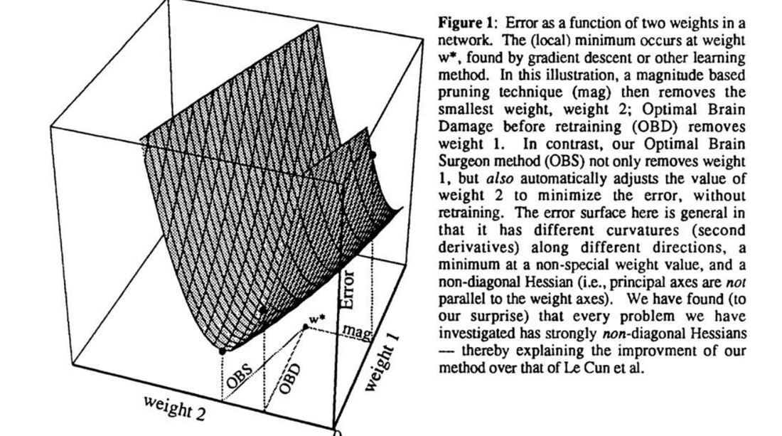
Source: Hassibi and Stork, Optimal Brain Surgeon, Figure 1. The crop preserves the paper’s own caption; this article uses it only to distinguish uncompensated and compensated deletion.

At Transformer scale, an exact full Hessian and inverse are generally impractical. Implementations use layerwise reconstruction objectives, Gauss-Newton/Fisher-like approximations, blocks, damping, factorizations, or sequential updates. If curvature is indefinite, singular, stale, or estimated from narrow calibration data, the clean quadratic interpretation weakens. Loop 3 will derive the scalable reconstruction path used by SparseGPT rather than pretending it materializes a model-wide exact Hessian.

0x02F Movement Is A Training-Trajectory Score

Movement pruning introduces score $S_i$ and forms a hard top-budget mask

$$M=\operatorname{TopBudget}(S).$$

The forward uses $\widehat W=M\odot W$. Because hard top selection has zero or undefined ordinary derivatives, the hard variant uses a straight-through estimator for the score path. The approximate derivative is

$$\frac{\partial\mathcal L}{\partial S_i} \approx \frac{\partial\mathcal L}{\partial M_i} = \frac{\partial\mathcal L}{\partial\widehat W_i}W_i =g_iW_i.$$

Gradient descent on the score gives

$$S_i^{(t+1)} = S_i^{(t)} - \eta_Sg_i^{(t)}W_i^{(t)}.$$

If a positive weight receives a negative gradient, its next weight update moves it farther positive; $g_iW_i<0$, so its score increases. The same holds for a negative weight receiving a positive gradient and moving farther negative. Thus a high accumulated score indicates movement away from zero under the fine-tuning objective, not simply a large final magnitude.

This score cannot be reconstructed from the final checkpoint alone. It depends on optimizer trajectory, batches, learning rate, score initialization, mask schedule, and straight-through approximation. Section 0x08 compares hard and soft movement, learned gates, gradual schedules, and exact-budget enforcement. Here, movement appears only to establish that when the evidence was collected is part of the evidence contract.

0x02G Learned Gates Optimize A Different Training Problem

Instead of computing one fixed score from a checkpoint, a method can attach a gate $z_G$ to every removable group and learn gate parameters $\phi_G$ jointly with model parameters. A generic stochastic objective is

$$\min_{\theta,\phi} \mathbb E_{z\sim q_\phi} \mathbb E_{x\sim\mathcal D} \left[ \mathcal L(x;\theta,z) \right] + \lambda \sum_G c_G\,\Pr_\phi(z_G\ne0),$$

where $c_G$ can represent one unit, parameter count, FLOPs, bytes, or another resource proxy. The second term is an expected resource penalty, not necessarily an exact deployed budget.

The discrete gate is not ordinarily differentiable. Hard-concrete methods replace it during optimization with a reparameterized stochastic relaxation, then clip or threshold to obtain zeros. Voita et al. applied stochastic head gates and a differentiable $L_0$ relaxation in their NMT head-pruning study. Their observation that specialized heads survived longer is source-scoped evidence about that trained setting, not proof that linguistic specialization is a universal pruning score.

Gate-based selection has several design choices:

gate one scalar, one head, one channel, one layer, or one coupled group
freeze or update base weights
stochastic sample or deterministic expectation in the forward pass
temperature/relaxation schedule
uniform L0 count or hardware/resource-weighted cost
threshold, top-budget projection, or constrained optimization at export

A gate probability of $0.2$ is not a final mask, and a sparsity penalty does not guarantee an exact target width. The export rule can change the ranking learned under the relaxed objective. Section 0x08 derives the relaxation and schedule mechanics in full.

0x02H Global, Local, Normalized, And Cost-Aware Rankings Differ

Even fixed evidence does not determine a mask until a budget rule is chosen. Let $I_G$ be retained importance and $C_G$ the deployment cost of keeping group $G$. A conceptual budget problem is

$$\max_{m_G\in\{0,1\}} \sum_Gm_GI_G \quad \text{subject to} \quad \sum_Gm_GC_G\le B.$$

If all groups have equal cost and additive independent importance, keeping the largest scores solves this approximation. Structured Transformer groups do not generally have equal cost. One residual channel propagates across many matrices; one head changes several projections; one layer removes an entire block. Ranking by $I_G/C_G$ is a useful greedy heuristic, not an exact solution to a discrete knapsack problem and not a model-quality theorem.

The ranking scope also matters:

Rule	Constraint	Benefit	Failure mode
tensor-local	keep a fixed fraction in every tensor	prevents one tensor from being emptied	ignores cross-tensor redundancy and cost
layer-local	allocate within one block	preserves broad depth coverage	can spend equal budget on unequal layers
global raw score	compare all candidate units directly	can learn nonuniform sparsity	score scales and group sizes may be incomparable
global normalized	normalize within layer/tensor, then compare	reduces scale imbalance	normalization removes potentially meaningful absolute sensitivity
cost-aware	include bytes/FLOPs/latency proxy	targets a resource	proxy may not match measured runtime
constrained candidate search	evaluate target shapes or subsets	handles interactions more directly	expensive and still data/workload dependent

Molchanov et al. and Michel et al. discuss layer-wise normalization because raw Taylor scales can vary across layers. Movement Pruning compares local and global top-budget masks. None of those empirical choices supplies a universal normalization. The score manifest must record the ranking pool, normalization, tie-breaking rule, and exact cost model.

0x02I One Matrix, One Removal Budget, Six Different Answers

Consider a didactic matrix with six scalar candidates:

$$W= \begin{bmatrix} 0.05 & 0.30 & 0.20\\ 0.10 & 0.40 & 0.25 \end{bmatrix}.$$

Let calibration input RMS by column be

$$r=[5.0,\ 0.1,\ 2.0],$$

and let one illustrative gradient estimate be

$$g= \begin{bmatrix} 2.00 & 0.50 & 0.01\\ 1.00 & 0.02 & 0.80 \end{bmatrix}.$$

Label entries row-major as $a,b,c,d,e,f$. For a diagonal-curvature teaching example use

$$\operatorname{diag}(H) =[200,\ 5,\ 5,\ 1,\ 1,\ 10].$$

Suppose accumulated movement scores and measured single-entry ablation loss changes are

$$S=[0.40,\ 0.20,\ 0.30,\ 0.50,\ 0.10,\ -0.20],$$ $$\Delta^{abl} =[0.09,\ 0.04,\ 0.02,\ 0.03,\ -0.01,\ 0.12].$$

Under a budget that removes exactly one entry:

Evidence	Score vector for a-f	Smallest / removed	Why
magnitude	[.05, .30, .20, .10, .40, .25]	a	smallest absolute weight
activation-weighted	[.25, .03, .40, .50, .04, .50]	b	column 2 is rarely energetic
instant Taylor	[.10, .15, .002, .10, .008, .20]	c	small current loss sensitivity
OBD diagonal	[.25, .225, .10, .005, .08, .3125]	d	flattest weighted coordinate
direct ablation	[.09, .04, .02, .03, -.01, .12]	e	removal lowered measured loss
movement	[.40, .20, .30, .50, .10, -.20]	f	lowest retained trajectory score

The arrays are a constructed counterexample, not a reported empirical result. Their purpose is to disprove the idea that a sparsity budget uniquely defines the mask. Each ranking is internally consistent with its own evidence, yet all six choose differently.

The disagreement is not a defect to average away blindly. It identifies which assumption needs validation:

magnitude -> parameter scale
activation -> calibration feature energy
Taylor -> local task-loss slope
curvature -> local quadratic geometry and compensation assumption
ablation -> measured one-unit intervention
movement -> fine-tuning trajectory

0x02J Tensor Hooks Must Preserve The Intended Reduction

For a linear weight $W[d_{out},d_{in}]$, activation statistics live on the input axis and scalar magnitude/Taylor statistics live on the full matrix:

class LinearEvidence:
    def __init__(self, weight):
        self.input_sumsq = zeros(weight.shape[1], dtype=float64)
        self.input_count = 0
        self.taylor_abs_sum = zeros_like(weight, dtype=float64)
        self.taylor_examples = 0

    def observe_input(self, x, valid_token_mask=None):
        # Flatten batch/sequence only after excluding padding or invalid tokens.
        rows = select_valid_rows(x, valid_token_mask).to(float64)
        self.input_sumsq += (rows * rows).sum(dim=0).cpu()
        self.input_count += rows.shape[0]

    def observe_microbatch_gradient(self, weight, microbatch_examples):
        # grad is for this microbatch reduction, not a stale accumulated grad.
        g = weight.grad.detach().to(float64)
        self.taylor_abs_sum += (
            (g * weight.detach()).abs().cpu() * microbatch_examples
        )
        self.taylor_examples += microbatch_examples

    def finalize(self, weight):
        rms = sqrt(self.input_sumsq / self.input_count)       # [d_in]
        magnitude = weight.detach().abs().cpu()               # [d_out, d_in]
        activation_weighted = magnitude * rms[None, :]        # broadcast input axis
        taylor_microbatch = self.taylor_abs_sum / self.taylor_examples
        return magnitude, activation_weighted, taylor_microbatch

This trace intentionally says microbatch. If the loss is mean-reduced over 32 examples, taking one absolute value after its backward pass measures the absolute gradient of that 32-example mean. It does not equal the mean of 32 per-example absolute gradients. Smaller microbatches reduce cancellation but increase overhead and still define another estimator.

For a structured group, an explicit gate is safer than guessing how scalar scores should be aggregated:

def gate_sensitivity(model, batch, groups):
    z = ones(len(groups), requires_grad=True)

    def loss_for_one(z_value, sample):
        output = model.forward_with_structural_gates(
            sample.inputs[None, ...], z_value, groups
        )
        return objective(output, sample.targets[None, ...], reduction="sum")

    # Conceptual torch.func-style vectorized gradient: [batch, groups].
    dz_per_example = vmap(grad(loss_for_one), in_dims=(None, 0))(z, batch)
    expected_abs = dz_per_example.abs().mean(dim=0)
    abs_expected = dz_per_example.mean(dim=0).abs()
    return expected_abs, abs_expected

The two returned vectors are both valid statistics, but they are not the same statistic. Code, formula, and prose must agree about which one drives pruning.

Distributed collection adds another reduction boundary. Averaging one local mean per rank is correct only when every rank contributes the same denominator. The replayable contract reduces sufficient statistics instead:

@dataclass
class ScoreSufficientStatistics:
    input_sumsq: Tensor          # [d_in], fp64 teaching accumulator
    valid_input_rows: int
    taylor_abs_sum: Tensor       # [d_out, d_in]
    taylor_signed_sum: Tensor    # [d_out, d_in]
    taylor_examples: int


def merge_score_shards(shards):
    # Conceptually all_reduce SUM on every numerator and denominator.
    input_sumsq = sum(s.input_sumsq for s in shards)
    valid_rows = sum(s.valid_input_rows for s in shards)
    taylor_abs = sum(s.taylor_abs_sum for s in shards)
    taylor_signed = sum(s.taylor_signed_sum for s in shards)
    examples = sum(s.taylor_examples for s in shards)

    return {
        "input_rms": sqrt(input_sumsq / valid_rows),
        "expected_abs_taylor": taylor_abs / examples,
        "abs_expected_taylor": abs(taylor_signed / examples),
    }

This is not merely a distributed-performance choice. For shard sizes one and four, mean(local_mean) weights the one-example shard and four-example shard equally; sum(local_numerator) / sum(local_count) reconstructs the monolithic estimator. The valid-token denominator must replace the example denominator when the objective and hook are token-reduced.

0x02K Evidence Needs A Provenance Manifest

Scores should not be serialized as anonymous tensors:

@dataclass
class ScoreManifest:
    method: str
    removable_unit: str
    tensor_axes: dict
    counterfactual: str
    hook_location: str | None
    hook_quantity: str | None
    checkpoint_hash: str
    checkpoint_step: int | None
    objective: str
    dataset_hash: str | None
    ordered_sample_ids_hash: str | None
    example_count: int | None
    valid_token_count: int | None
    valid_row_policy: str | None
    batch_or_microbatch_size: int | None
    reduction: str
    reduction_order: str
    parameter_state: str       # initialization, pretrained, fine-tuning step, final
    compensation: str          # none, diagonal, inverse-curvature, reconstruction
    group_aggregation: str
    normalization: str
    ranking_scope: str         # tensor, layer, global
    cost_model: str | None
    target_budget: dict
    tie_break: str
    random_seed: int | None
    model_mode: str            # eval/train; records dropout and stochastic layers
    source_dtype: str
    accumulator_dtype: str
    world_size: int
    distributed_reduction: str | None
    trajectory_hash: str | None
    relaxation: dict | None
    score_tensor_hash: str

For magnitude, data fields may be null. For activation/Taylor/ablation, they are correctness state. For movement, the final score tensor is insufficient; the training and mask schedules also belong to lineage. For a learned gate, relaxation, temperature, penalty, and export threshold must be added.

The manifest also closes a subtle provenance gap between where a quantity is observed and what it means:

Evidence	Required hook or state	Axis before reduction	Reduction that must remain visible
magnitude	checkpoint parameter	full parameter tensor	elementwise absolute value, then named group/ranking reduction
activation-weighted	linear input before the projection	input-feature axis plus valid calibration rows	sum of squares and count, then square root; raw $L_2$ or RMS named
scalar Taylor	parameter gradient plus the parameter, or an explicit scalar gate	full parameter tensor	per-example/microbatch absolute placement named
structured Taylor	one gate at the actual removable group output	group gate axis	sum inside the shared perturbation before absolute value
diagonal curvature	diagonal curvature estimate and matching parameter state	selected parameter coordinate	no off-diagonal compensation may be implied
movement	score/weight/gradient trajectory at every scored update	score tensor and time	ordered update accumulation; final checkpoint alone is insufficient
learned stochastic gate	gate distribution parameters and random state	declared structural gate	expected active probability is not an exact exported budget
direct ablation	controlled model evaluation with one frozen intervention	candidate unit	baseline and ablated numerators/counts under the same sample order

The Loop 2 oracle uses an uneven two-shard split deliberately. It proves that the sufficient-statistic merge reproduces the monolithic score, while an unweighted mean of shard means does not. It also computes both $\mathbb E[|gw|]$ and $|\mathbb E[gw]|$, and both the shared-gate Taylor score and the sum of scalar absolute scores, so none of those pairs can pass as aliases.

0x02L Score Failure Lab

Failure	Silent cause	Observable consequence	Repair
compute absolute value after averaging examples	positive and negative sensitivities cancel	units look unimportant despite high per-example sensitivity	state the reduction; use per-example or controlled microbatch statistics
compare raw magnitude across rescaled equivalent layers	score is not invariant to parameter scaling	global mask follows scale convention	prune locally or use validated normalization/functional evidence
rank unequal groups by raw $L_2$ norm	larger groups accumulate larger norm	small groups are removed disproportionately	normalize for group size or use a shared gate
capture activations on unrelated short prompts	calibration misses deployment states	selected mask fails on target domain/length	stratify calibration and record token population
call raw calibration $L_2$ norm an RMS score	missing $\sqrt{N_{valid}}$ normalization	score magnitudes drift across calibration sizes even if one local ranking is unchanged	name raw $L_2$ versus RMS and persist the valid-row count
call activation magnitude task importance	downstream loss is absent	high-energy but cancelable features are protected	add gradient/ablation evidence or state local reconstruction target
use $	\mathbb E[gw]	$while documenting$\mathbb E[	gw
sum scalar Taylor values for a shared group without naming aggregation	cancellation semantics change	group score is implementation-dependent	gate the group directly or state sum/absolute convention
apply diagonal OBD formula and claim OBS compensation	off-diagonal inverse curvature omitted	recovery effect is overstated	name diagonal deletion versus compensated deletion
compute movement score only at final checkpoint	trajectory state is unavailable	score degenerates into another post-hoc proxy	collect scores during the specified fine-tuning run
treat learned gate probability as an exact budget	relaxed expected cost is not exported shape	final mask misses target width/cost	project or search under the exact target and reevaluate
prune many units using stale one-at-a-time ablations	unit interactions accumulate	joint quality collapses	recompute iteratively or evaluate candidate subsets
rank score only, ignoring group cost	equal score can buy different savings	pruning misses deployment objective	solve or approximate a stated cost-constrained selection problem
average rank-local score means	unequal shard denominators are hidden	score changes with world size or sampler partition	all-reduce sufficient-statistic numerators and counts
collect hooks with dropout active but replay in eval mode	stochastic model state is absent from provenance	repeated calibration produces another ranking	freeze and record model mode and random state

0x02M Loop Boundary

Loop 2 has established how pruning evidence is produced:

exact intervention -> direct but expensive and interaction-sensitive
zeroth order       -> cheap parameter proxy
activation         -> calibration-local functional perturbation
first order        -> objective slope under a named reduction
second order       -> local curvature, with or without compensation
movement/gates     -> training-time evidence with additional state

The next loop will hold the removal unit fixed at scalar weights inside one linear layer and compare three one-shot LLM paths: magnitude, Wanda’s activation-weighted per-output ranking, and SparseGPT’s layerwise reconstruction with compensating updates. That section will derive the shared reconstruction objective and show where the algorithms cease to be equivalent.

0x03 One-Shot Unstructured Pruning Is A Reconstruction Design Space

The word one-shot can suggest a cheap operation: compute one score, write zeros, and stop. That describes magnitude pruning and approximates Wanda’s selection path, but it does not describe SparseGPT. All three methods start from a trained checkpoint and avoid ordinary end-to-end retraining. They differ in the evidence they collect, the scope over which they allocate zeros, and whether retained weights may move to repair the local function.

The owner question for this loop is:

Given calibration inputs to one linear layer, should pruning preserve the original parameters, preserve each output approximately without weight updates, or solve a sparse reconstruction with compensating weight updates?

This section owns scalar unstructured masks, calibration statistics, local reconstruction, and the sequential layerwise compression process. It does not claim that an ordinary dense checkpoint with zeros executes fewer operations. Loop 4 owns N:M layout and sparse-kernel eligibility. Loops 5-7 own physically smaller head, width, and depth artifacts. Section 0x08 owns training-time scores, gates, budgets, and schedules; Loop 10 owns the cross-method recovery comparison.

Loop 3 accompanies this prose with a deterministic small-matrix reconstruction fixture. It does not execute PyTorch, a Transformer checkpoint, the SparseGPT or Wanda repositories, a GPU, or a sparse runtime. It does replay the algebraic contracts that must agree before those larger claims are meaningful:

fixed support least squares
    <-> exact OBS deletion of only the masked coordinates

SparseGPT fixed-mask eager update
    <-> SparseGPT fixed-mask lazy block update

Wanda metric and per-output allocation
    <-> exact mask-only zero artifact

dense upstream hidden states
    != hidden states propagated through the pruned upstream layer

The fixture freezes W, X, orientation, valid calibration rows, objective scale, damping, factorization convention, column order, mask-selection scope, tie policy, update schedule, block sizes, output dtype, and artifact identity. Its claim ceiling remains synthetic teaching evidence: paper quality, framework fidelity, kernel execution, and deployment speed remain unclaimed.

0x03A The Shared Objective Is Sparse Regression On Layer Inputs

Let one linear layer have

$$W\in\mathbb R^{d_{out}\times d_{in}}, \qquad X\in\mathbb R^{d_{in}\times n}, \qquad Y=WX.$$

Each column of $X$ is one calibration activation vector. In a Transformer, batch and valid sequence positions are normally flattened into the sample axis $n$ after padding and excluded positions are handled. Let binary mask $M$ use $1$ for retained entries, and let $W_c$ denote values permitted after compression. The layerwise pruning problem is

$$\min_{M,W_c} \left\| WX-(M\odot W_c)X \right\|_F^2 \quad\text{subject to a sparsity constraint on }M.$$

This is already more specific than “remove small weights.” It says:

• the dense layer output on calibration inputs is the teacher target;
• the mask and possibly changed surviving values define the student layer;
• error is measured before later nonlinearities repair or amplify it;
• the sparsity constraint defines where selection is allowed to compete.

Jointly choosing the discrete mask and continuous reconstruction is a sparse regression problem and is NP-hard in general. Practical methods change the problem:

magnitude:
    choose M from abs(W); keep W_c = W

Wanda:
    choose M from abs(W_ij) * input_norm_j; keep W_c = W

SparseGPT:
    choose M adaptively from reconstruction evidence;
    update still-unfrozen entries of W_c to compensate

To expose the geometry, define

$$\Delta W=W-M\odot W_c, \qquad G=XX^T.$$

Then

$$\|\Delta W X\|_F^2 = \operatorname{tr}(\Delta W G\Delta W^T) = \sum_{i=1}^{d_{out}} \Delta w_iG\Delta w_i^T.$$

The reconstruction decomposes by output row because every row shares the same input Gram matrix $G$ but has its own weight vector and mask. This row separability enables parallel arithmetic. It does not imply that every row has the same optimal mask.

For an average-squared objective it is convenient to define

$$H=\frac{2}{n}XX^T,$$

so one row’s reconstruction cost is

$$\mathcal E_i(\delta w_i) = \frac{1}{2}\delta w_iH\delta w_i^T.$$

Factors of $2$ and $n$ vary between papers and code. They change reported error scale but not an undamped ranking under one shared factor. Damping and mixed normalization do change the solution and must be recorded.

0x03B A Fixed Mask Is Easy Algebraically But Expensive Row By Row

Suppose the retained input-coordinate set for output row $i$ is $K_i$. Let

$$y_i=w_iX\in\mathbb R^{1\times n}$$

be the original dense output and let $X_{K_i}$ contain the retained input rows. Once the mask is fixed, the best reconstructed retained row solves

$$\min_{u_i} \|y_i-u_iX_{K_i}\|_2^2.$$

The normal equation is

$$u_iX_{K_i}X_{K_i}^T = y_iX_{K_i}^T,$$

giving, when the system is invertible,

$$u_i^* = y_iX_{K_i}^T \left(X_{K_i}X_{K_i}^T\right)^{-1}.$$

A damped or pseudoinverse solution is needed when calibration features are rank-deficient. The costly part is not writing this formula. Different rows usually retain different $K_i$, so they require inverses of different masked Gram matrices. In general,

$$\left(G_{K_i,K_i}\right)^{-1} \ne \left(G^{-1}\right)_{K_i,K_i}.$$

Masking an inverse is not the inverse of the masked system. Recomputing a $d_{in}\times d_{in}$-scale inverse independently for every output row would destroy the scalability gained from row separability. SparseGPT’s central systems idea is to share one elimination sequence across rows even though the rows freeze different values to zero.

0x03C OBS Shows What A Compensating Deletion Must Do

For one row, let $q$ be the coordinate to remove and let $e_q$ be its basis vector. Under the quadratic reconstruction objective, deletion requires

$$e_q^T\delta w+w_q=0.$$

The constrained optimum derived in 0x02E is

$$\delta w^* = -\frac{w_q}{[H^{-1}]_{qq}}H^{-1}e_q,$$

with reconstruction increase

$$\epsilon_q = \frac{1}{2} \frac{w_q^2}{[H^{-1}]_{qq}}.$$

The $q$ component of the update is exactly $-w_q$, making the deleted weight zero. Off-diagonal entries of $H^{-1}e_q$ move correlated survivors. Without those entries, deletion changes the local function more.

Consider a two-feature teaching system:

$$H= \begin{bmatrix} 2&1\\ 1&2 \end{bmatrix}, \qquad H^{-1}=\frac{1}{3} \begin{bmatrix} 2&-1\\ -1&2 \end{bmatrix}, \qquad w=[0.2,1.0].$$

Deleting the first weight without compensation uses

$$\delta w_{zero}=[-0.2,0], \qquad \mathcal E(\delta w_{zero})=0.04.$$

OBS instead gives

$$\delta w^*=[-0.2,0.1], \qquad w+\delta w^*=[0,1.1],$$

and

$$\mathcal E(\delta w^*)=0.03.$$

The removed coordinate is still zero. The lower error comes from changing the surviving coordinate. This is the distinction between mask-only pruning and local reconstruction, not evidence that any arbitrary update improves the full model.

Sequentially applying exact OBS updates can recover the exact optimum for a fixed final mask in this quadratic row problem when the algorithm eliminates only coordinates in that mask and keeps every surviving coordinate available for compensation until all deletions finish. Freezing an unpruned coordinate merely because its column was visited removes that coordinate from later compensation and changes the optimization problem. The direct exact path is still too expensive at LLM dimensions because each row mask induces its own active inverse. SparseGPT changes which coordinates remain updateable so one inverse-Hessian sequence can be shared across rows; it is an efficient ordered partial reconstruction, not an alias for independently solving every row’s fixed-support least-squares system.

0x03D SparseGPT Synchronizes Elimination, Not Row Masks

SparseGPT fixes an input-coordinate order

$$1,2,\ldots,d_{in}$$

and defines an active suffix $U_j$ containing coordinate $j$ and all later coordinates. After processing $j$, that coordinate is frozen: it is either zero or retained at its current reconstructed value, and later updates may touch only the remaining suffix.

Let

$$B_j=\left(H_{U_j,U_j}\right)^{-1}.$$

After eliminating the first coordinate of the active system, the next inverse can be obtained by one Schur-complement/Gaussian-elimination step:

$$B_{j+1} = \left( B_j- \frac{B_j[:,1]B_j[1,:]}{B_j[1,1]} \right)_{2:,2:}.$$

Every output row uses this same sequence because $H$ depends only on layer inputs. Rows can still choose different weights to zero. At a processed column $j$:

row where M[i,j] = 0:
    set the current reconstructed value to zero
    emit a compensation error into later columns

row where M[i,j] = 1:
    freeze the current reconstructed value
    emit zero pruning error

This is why “shared Hessian” must not be rewritten as “shared mask.” The algorithm synchronizes the elimination order and inverse-curvature state, not the row-level keep/drop decisions.

SparseGPT also selects masks adaptively in column blocks. At the start of a selection block, it ranks current reconstructed weights using predicted pruning error independently within each output row, matching the reference implementation’s topk(..., dim=1) allocation axis. It then performs the block’s updates before selecting the next mask block, allowing earlier compensation to influence later decisions. The paper distinguishes:

• $B_s$: columns considered together when allocating the block sparsity;
• $B$: columns whose updates are accumulated before one lazy matrix update.

They are algorithmic batching controls, not the deployed sparse layout. Loop 4 will treat an N:M group as a separate artifact constraint.

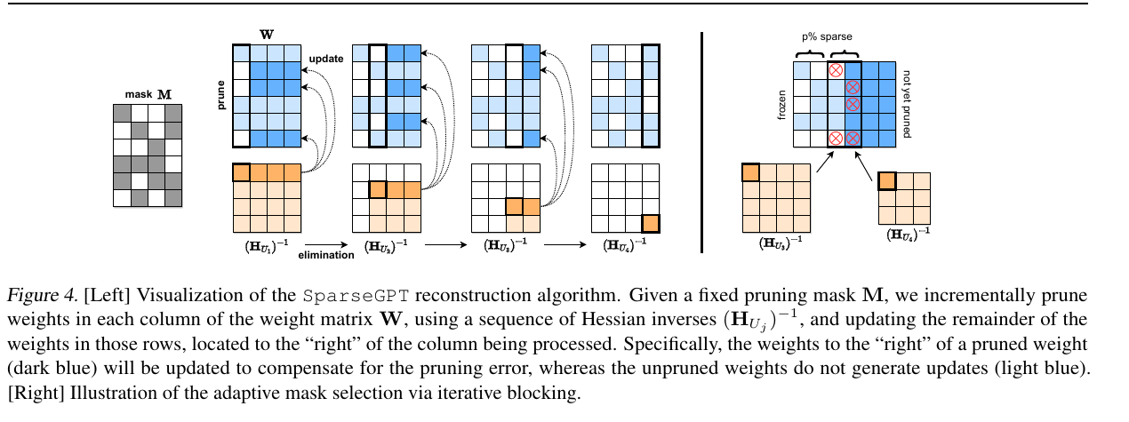
Source figure: Frantar and Alistarh, SparseGPT, Figure 4, extracted from the revision-pinned 2301.00774v3 PDF. The left panel distinguishes the row mask from the shared column-elimination sequence; the right panel shows that mask selection is refreshed by blocks. The figure explains the paper algorithm and does not constitute a reproduced pruning result.

0x03E The Cholesky Code Path Is Not The Raw OBS Formula

The official implementation first accumulates a scaled input Gram matrix, handles input coordinates with zero observed energy, applies diagonal damping, inverts the system, and stores an upper Cholesky factor of that inverse:

$$H_\lambda = \frac{2}{n}XX^T+\lambda I, \qquad R^TR=H_\lambda^{-1}.$$

The reference code uses a relative damping value

$$\lambda = \rho\,\operatorname{mean}(\operatorname{diag}H),$$

with $\rho$ supplied as percdamp. Damping improves numerical conditioning but changes the reconstruction geometry. It is not a harmless implementation detail.

During ordered elimination, the code uses

$$d_j=R_{jj}.$$

For a current weight vector $w=W[:,j]$ and frozen value $q$ (zero for pruned rows, current value for kept rows), it forms

$$e_j=\frac{w-q}{d_j}$$

and applies

$$W[:,j:] \leftarrow W[:,j:]-e_jR[j,j:].$$

The mask score used by the implementation is proportional to

$$S_{ij}^{SGPT} = \frac{W_{ij}^2}{R_{jj}^2}$$

for the current selection state. $R_{jj}^2$ should not be casually labeled the original raw diagonal of $H^{-1}$. It is the diagonal factor consumed by the ordered Cholesky/elimination procedure. The paper reuses inverse-Hessian notation around this factorized algorithm; code-level explanations should name which object is actually indexed.

A faithful teaching sketch is:

def sparsegpt_linear(weight, calibration_inputs, sparsity,
                     lazy_block=128, mask_block=128, damp_ratio=0.01):
    # weight: [d_out, d_in]
    # X:      [d_in, valid_calibration_tokens]
    X = flatten_valid_tokens(calibration_inputs).T.float()
    H = (2.0 / X.shape[1]) * (X @ X.T)                 # [d_in, d_in]

    dead = diag(H) == 0
    weight[:, dead] = 0
    H[dead, dead] = 1
    H += damp_ratio * mean(diag(H)) * eye(H.shape[0])

    Hinv = inverse_from_cholesky(H)
    R = upper_cholesky(Hinv)                           # R.T @ R = Hinv
    W = weight.float().clone()
    Q = zeros_like(W)

    for block_start in range(0, W.shape[1], lazy_block):
        block_end = min(block_start + lazy_block, W.shape[1])
        block_errors = zeros(W.shape[0], block_end - block_start)

        for j in range(block_start, block_end):
            if starts_new_mask_block(j, mask_block):
                cols = current_mask_block(j, mask_block, W.shape[1])
                score = W[:, cols].square() / diag(R)[cols].square()[None, :]
                mask = lowest_fraction_per_output_row(score, sparsity, dim=1)

            current = W[:, j]
            frozen = current.clone()
            frozen[mask[:, j]] = 0
            Q[:, j] = frozen

            error = (current - frozen) / R[j, j]
            W[:, j:block_end] -= error[:, None] * R[j, j:block_end][None, :]
            block_errors[:, j - block_start] = error

        # Lazy update gives the same accumulated block correction to the tail.
        W[:, block_end:] -= block_errors @ R[block_start:block_end, block_end:]

    return Q

This is mechanism pseudocode, not a drop-in reimplementation. Production code must define exact block boundaries, stable threshold/tie behavior, transposed Conv1D storage, dtype restoration, device placement, and optional joint quantization. The final zero pattern still needs an executable sparse format and kernel before it becomes acceleration.

0x03F Wanda Keeps The Diagonal Perturbation And Drops Reconstruction

Wanda begins from the no-compensation perturbation derived in 0x02D. For one row,

$$y_i=\sum_jW_{ij}x_j.$$

Deleting a set $P_i$ changes the output by

$$\delta y_i = -\sum_{j\in P_i}W_{ij}x_j.$$

Its squared calibration norm is

$$\|\delta y_i\|_2^2 = \sum_{j\in P_i}W_{ij}^2\|X_j\|_2^2 + 2\sum_{j<k;\,j,k\in P_i} W_{ij}W_{ik}\langle X_j,X_k\rangle.$$

Wanda uses the individual diagonal term’s square root:

$$S_{ij}^{Wanda} = |W_{ij}|\,\|X_j\|_2.$$

It ignores the cross-feature terms and performs no compensating update. This makes the method much cheaper than inverse-curvature reconstruction, but also states its approximation clearly: correlated deletion errors are not solved jointly.

The input norm has shape $[d_{in}]$ and is broadcast over output rows:

$$|W|[d_{out},d_{in}] \odot \|X\|_{feature}[1,d_{in}] \rightarrow S[d_{out},d_{in}].$$

For unstructured sparsity ratio $p$, Wanda sorts each output row and removes

$$k=\lfloor p\,d_{in}\rfloor$$

lowest scores in that row. Per-output ranking is part of the method, not a cosmetic implementation choice. It ensures every output retains the same number of incoming connections. A global threshold could spend most zeros in a few output rows; a layer-global magnitude baseline and a row-local Wanda mask therefore differ in both metric and allocation scope.

Consider

$$W= \begin{bmatrix} 0.05&0.10&0.05\\ 0.50&0.60&0.70 \end{bmatrix}, \qquad \|X_j\|_2=[4.0,0.2,1.0].$$

Wanda scores are

$$S= \begin{bmatrix} 0.20&0.02&0.05\\ 2.00&0.12&0.70 \end{bmatrix}.$$

At one removal per output, both rows remove the second input connection. The first feature’s high calibration energy protects even the first row’s small $0.05$ weight. A global two-entry budget would remove scores $0.02$ and $0.05$ from the first row, leaving the second row dense. Same score tensor, different allocation contract, different mask.

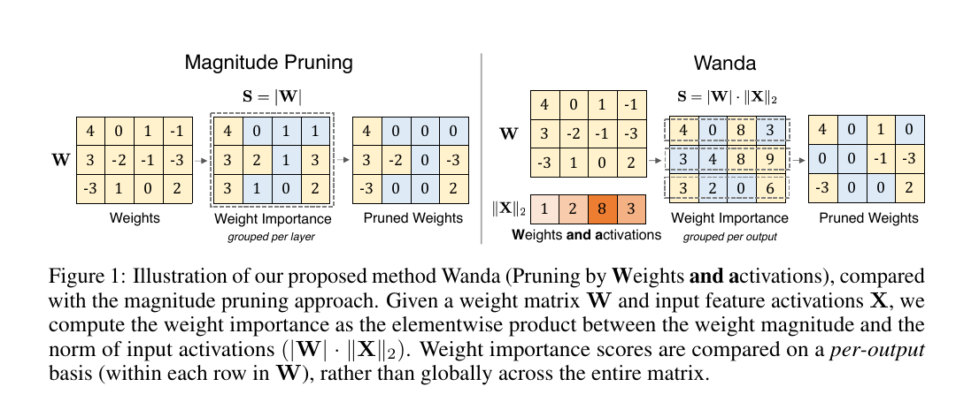
Source figure: Sun et al., Wanda, Figure 1, extracted from the revision-pinned 2306.11695v3 PDF. It makes two changed objects visible at once: the score uses input-feature activation norms, and the allocation scope changes from one layer-wide pool to independent per-output rows. The shown example is paper-local explanatory evidence, not a universal quality claim.

0x03G The Wanda Hook And Mask Axis Must Agree

The official implementation flattens sequence positions, transposes the input to [d_in, token_positions], and accumulates squared feature norms over calibration examples. Its stored scaler_row is named from an older wrapper, but its length is the input-column count, not the output-row count. The square root is taken before broadcasting into the weight metric.

A clearer equivalent trace is:

class WandaInputNorm:
    def __init__(self, d_in):
        self.sequence_sumsq_mean = zeros(d_in, dtype=float64)
        self.sequence_count = 0

    def add_batch(self, x, valid_token_mask=None):
        # x: [batch, sequence, d_in]
        # Preserve a named population; do not silently include padding.
        for sequence, mask in zip(x, valid_token_mask):
            rows = sequence[mask].to(float64)
            sequence_sumsq = rows.square().sum(dim=0)  # [d_in]
            self.sequence_sumsq_mean = online_mean(
                self.sequence_sumsq_mean,
                self.sequence_count,
                sequence_sumsq,
            )
            self.sequence_count += 1

    def score_and_mask(self, weight, sparsity):
        input_norm = sqrt(self.sequence_sumsq_mean)       # [d_in]
        score = weight.abs() * input_norm[None, :]        # [d_out, d_in]
        k = floor(weight.shape[1] * sparsity)
        prune_idx = stable_argsort(score, dim=1)[:, :k]   # sort each output row
        mask = zeros_like(weight, dtype=bool)
        mask.scatter_(dim=1, index=prune_idx, value=True)
        return score, mask

Averaging per-sequence squared norms differs from one total token norm only by a common factor, whatever the valid lengths: the mean of $N$ per-sequence sums is the sum over all valid tokens divided by $N$. It therefore does not change row rankings, and the official WrappedGPT.add_batch keeps the same kind of quantity: the squared-norm total over the positions it receives, divided by the number of calibration sequences. An accumulator that first divided each sequence by its own length would give short sequences’ tokens more weight and could change row rankings when lengths vary; this one does not. Padding inclusion, packed samples, and prompt-domain mixtures change which tokens are measured, not that proportionality. The calibration manifest must say what population produced $\|X_j\|_2$.

After mask creation, reference Wanda writes exact zeros:

weight[mask] = 0

There is no reconstruction update and no backward pass. Optional later LoRA or full recovery is a different pipeline. Calling a recovered Wanda checkpoint “Wanda with no updates” would erase an important experimental distinction.

0x03H Sequential Layer Processing Changes The Calibration State

Both reference pipelines process Transformer blocks in order to limit memory. The orchestration is more involved than running independent hooks on the original dense model:

1. disable generation KV caching;
2. capture the first block's hidden-state inputs for calibration sequences;
3. retain attention masks, position IDs, and other required block state;
4. for block l:
       run current block on current inputs with linear hooks;
       collect input norms or Gram/Hessian state;
       prune the selected linear modules;
       rerun the now-pruned block;
       use those outputs as block l+1 calibration inputs;
5. restore model configuration and serialize pruning provenance.

The first pass through block $l$ measures its dense sublayers under the hidden states produced by already-pruned blocks $<l$. The second pass propagates the new block error forward. Thus later layers are calibrated on a progressively compressed upstream model, not necessarily on hidden states cached once from the original dense model.

A state-safe teaching skeleton is:

@no_grad()
def sequential_one_shot(model, calibration_batches, method):
    previous_use_cache = model.config.use_cache
    model.config.use_cache = False
    try:
        inps, attention_mask, position_ids = capture_first_block_inputs(
            model, calibration_batches
        )

        for layer_id, block in enumerate(model.layers):
            block_device = device_for_block(model, layer_id)
            inps = inps.to(block_device)

            collectors = register_linear_input_collectors(block, method)
            dense_outs = run_block_samples(
                block, inps, attention_mask, position_ids
            )
            remove_hooks(collectors)

            for name, linear in ordered_target_linears(block):
                if method == "wanda":
                    score, mask = collectors[name].wanda_mask(linear.weight)
                    linear.weight[mask] = 0
                elif method == "sparsegpt":
                    linear.weight = collectors[name].sparsegpt_reconstruct(
                        linear.weight
                    )

            pruned_outs = run_block_samples(
                block, inps, attention_mask, position_ids
            )
            inps = pruned_outs
            free_layer_collectors(collectors)
    finally:
        model.config.use_cache = previous_use_cache

dense_outs is shown to distinguish the statistics pass, but it need not be retained after pruning if memory is constrained. Real model blocks may require rotary position state, cache-position arguments, cross-attention inputs, or architecture-specific projection orientation. Catching the first block by raising a generic exception is a convenient reference-code technique, not a recommended production control-flow API.

0x03I Calibration Memory Is Part Of Method Cost

For $N$ calibration sequences of length $S$, hidden width $d$, and element size $b_h$, one hidden-state buffer costs

$$M_{hidden}=NSd\,b_h.$$

With $N=128$, $S=2048$, $d=4096$, and FP16 storage:

$$M_{hidden}=2\ \text{GiB}.$$

Separate input and output buffers therefore consume about $4$ GiB before model weights, hooks, and solver state. Streaming or smaller calibration batches can lower residency, but then accumulation order and host/device transfer become part of the implementation.

Wanda’s persistent statistic for one linear layer is only

$$M_{Wanda\ stat}=d_{in}b_s,$$

where $b_s$ is the accumulator element size. SparseGPT stores a dense $d_{in}\times d_{in}$ reconstruction matrix:

$$M_H=d_{in}^2b_s.$$

At FP32 accumulator precision:

$d_{in}$	input-norm vector	dense $H$ or factor
4096	16 KiB	64 MiB
11008	43 KiB	about 462 MiB

Processing several linears’ collectors simultaneously multiplies this state. SparseGPT also pays approximately $O(nd_{in}^2)$ to accumulate the Gram matrix, $O(d_{in}^3)$ for factorization/elimination state, and $O(d_{out}d_{in}^2)$ for reconstruction updates. Lazy update blocks improve compute-to-memory behavior; they do not make the dense curvature state linear in $d_{in}$.

The paper’s calibration choice of 128 C4 segments of length 2048 and its reported runtimes are source-reported experimental settings, not universal defaults. Domain, tokenizer, sequence length, padding, and number of samples remain part of the released artifact’s evidence lineage.

0x03J Reconstruction Evidence Needs Its Own Manifest

A mask file alone cannot replay a one-shot reconstruction. The same mask can produce different survivor values under a different calibration population, damping rule, factorization, elimination order, block schedule, or dtype. A minimal evidence record is therefore method- and action-aware:

@dataclass(frozen=True)
class ReconstructionManifest:
    dense_checkpoint_sha256: str
    calibration_values_sha256: str
    ordered_sample_ids_sha256: str
    weight_shape: tuple[int, int]
    calibration_layout: str          # feature_by_valid_position
    objective: str                   # layer_output_squared_error
    objective_scale: str             # e.g. 2 / valid_positions
    accumulator_dtype: str
    dead_feature_policy: str
    damping_rule: str
    damping_ratio: float
    factorization: str               # upper_cholesky_of_inverse
    column_order: tuple[int, ...]
    selection_metric: str
    allocation_scope: str
    mask_refresh_schedule: str
    tie_policy: str
    survivor_update: str             # none, exact_obs, ordered_partial
    lazy_update_block_size: int
    selection_block_size: int
    output_dtype: str
    expected_mask_sha256: str
    expected_weight_sha256: str
    expected_dense_shape: tuple[int, int]
    runtime_format: str               # dense_tensor_with_exact_zeros

The Loop 3 fixture uses a 2 x 4 weight matrix and four input features over five calibration positions. It records separate masks for a fixed-support comparison, Wanda, and adaptive SparseGPT. Its executable oracle proves:

1. independently solved fixed-support least squares matches exact sequential OBS deletion to numerical tolerance;
2. SparseGPT’s ordered partial reconstruction is not silently relabeled as that exact row-specific solve;
3. adaptive SparseGPT removes the declared count independently per output row inside each selection block;
4. eager and lazy SparseGPT updates match for the same frozen mask, factor, order, and block boundaries;
5. the upper-factor diagonal consumed by code is not generally the raw diagonal of the inverse Gram matrix;
6. Wanda changes no surviving value and its per-output mask is reproduced from the recorded activation population;
7. propagated hidden states after pruning differ from dense cached hidden states, making sequential layer processing observable; and
8. every output remains an ordinary dense-shape tensor with exact zeros, so no runtime acceleration claim is admitted.

The oracle also rejects one-field mutations for transposed calibration axes, changed masks, reordered columns, missing damping, changed tie rules, mixed eager/lazy schedules, altered hashes, survivor-update aliasing, and promoted runtime or quality claims. That is evidence for the mechanism contract, not a substitute for evaluating a real model.

0x03K Selection, Reconstruction, And Recovery Are Three Separate Knobs

These methods should not be compared under labels that hide their update budgets:

Path	Calibration evidence	Mask allocation	Survivor update during pruning	Later recovery
magnitude mask-only	none	configured global/layer/tensor scope	none	optional, separate
Wanda reference	input feature norms	fixed fraction per output row	none	optional, separate
fixed-mask least squares / AdaPrune family	layer inputs and dense outputs	mask selected first	regression or SGD reconstruction	optional
OBC/OBQ-style greedy	inverse-curvature state	one decision at a time	exact local compensation under quadratic model	optional
SparseGPT	damped layer-input curvature	adaptive column blocks	ordered Cholesky/lazy compensation	optional
recovery fine-tuning	training data and objective	mask fixed or constrained	many optimizer steps	this row is recovery

“No retraining” does not mean “no data,” “no updates,” or “one forward evaluation.” SparseGPT changes retained weights without end-to-end gradient training. Wanda uses calibration data but leaves retained values untouched. Magnitude can be data-free but still needs a declared allocation scope.

The methods also optimize local output fidelity, not task quality directly. A lower $\|WX-\widehat W X\|_F^2$ on calibration data can correlate with better downstream behavior, but it does not prove equivalent generation, safety, factuality, long-context behavior, or latency. Those are independent evaluation gates.

0x03L Reconstruction Failure Lab

Failure	Silent cause	Observable consequence	Repair
use $X$ as [samples, d_in] in $XX^T$ without transposing	sample and feature axes swapped	Hessian shape follows token count or multiplication fails	assert X.shape == [d_in, n] before Gram accumulation
include padded tokens in activation norms	padding population differs across batches	Wanda scores follow sequence padding policy	mask invalid token rows before accumulation
call Wanda scaler_row an output statistic	wrapper name confused with tensor axis	norm is broadcast on wrong axis	assert statistic length equals weight.shape[1]
sort Wanda scores globally	allocation scope changed	some output rows lose many more connections	stable-sort along dim=1 for reference per-output pruning
use raw $\operatorname{diag}(H^{-1})$ while copying Cholesky update code	formula object and code object differ	mask and compensation do not reproduce reference path	name and test the upper factor $R$ used by elimination
omit damping on rank-deficient calibration features	inverse/factorization is unstable	NaNs, failed Cholesky, or extreme updates	record damping rule and dead-feature policy
reconstruct pruned coordinates again later	frozen-state invariant broken	zeros silently become nonzero	freeze processed columns and validate final mask
reuse one masked inverse for all row masks	inverse of submatrix assumed equal to submatrix of inverse	compensation is mathematically wrong	use synchronized elimination or solve each fixed mask correctly
select all SparseGPT masks before any compensation	adaptive state removed	later blocks ignore earlier updates	select masks at documented block boundaries
feed dense original hidden states to every later block	sequential propagation omitted	calibration no longer matches progressively pruned model	rerun each pruned block and propagate its outputs
leave use_cache=True during calibration	generation state leaks into block traversal	excess memory or architecture-specific cache behavior	disable and restore cache configuration with finally
report one-shot as zero-cost	factorization, updates, and two block passes omitted	deployment preparation estimate is wrong	publish calibration time, peak memory, and artifact conversion time
benchmark dense zero tensors as sparse execution	artifact remains ordinary dense	FLOPs and latency are unchanged	convert to supported format and inspect selected kernels in Loop 4
compare recovered Wanda with unrecovered SparseGPT	training budgets differ	method conclusion is confounded	separate selection, reconstruction, and recovery columns
call ordered partial SparseGPT reconstruction the exact row-wise least-squares optimum	retained earlier columns were frozen before later deletions	reported optimality exceeds the executed update set	compare against the fixed-support solve and record the updateable suffix at every step
publish only the zero mask	damping, order, factorization, and survivor values are absent	the reconstructed checkpoint cannot be replayed	publish the reconstruction manifest and final weight digest
average per-rank Gram matrices without sample-count weighting	calibration shards have different valid-position counts	factorization depends on world-size partitioning	reduce Gram numerators and valid counts, then normalize once

0x03M Loop Boundary

Loop 3 has followed the complete one-shot path:

calibration hidden states
    -> input norms or dense Gram/curvature state

mask allocation
    -> per-output Wanda ranking or adaptive SparseGPT blocks

weight action
    -> exact zeros only, or zeros plus compensating survivor updates

sequential propagation
    -> pruned block outputs become the next block's calibration inputs

artifact
    -> same dense tensor shapes with many zero entries

That last line is the handoff. Loop 4 will constrain zeros into N:M groups, derive value-plus-metadata storage, validate axis and shape eligibility, and prove whether an actual sparse kernel is selected. Loop 3 does not claim latency from an unstructured zero count.

0x04 N:M Sparsity Is A Local Mask, A Packed ABI, And A Kernel Decision

Unstructured pruning asks which scalar weights may become zero. N:M sparsity adds a stricter question: which zeros may coexist inside every small, hardware-visible group? That regularity sacrifices mask freedom in exchange for fixed work and compact location metadata. It still does not make the result executable by itself.

The owner question for this loop is:

How does a row-local N:M selection become a validated value-plus-metadata artifact, enter an eligible sparse matrix multiplication, and demonstrate a measured saving against the same pruned values executed densely?

This section uses N_keep:M to mean that exactly N_keep positions are selected in each logical group of M weight positions. Hardware and runtime documentation often phrases the same 2:4 constraint as “at least two zeros” or “at most two nonzeros.” Those statements are compatible for ordinary nonzero weights, but a compressed format still reserves a fixed number of value slots. A selected slot may numerically contain zero, so selected position count, numerical nonzero count, and stored value count must not be treated as synonyms.

There is also an API naming trap. The official SparseGPT and Wanda reference code accepts arguments named prunen and prunem, where prunen is the number of entries zeroed in each group. This article’s N_keep is the number retained:

$$N_{prune}=M-N_{keep}.$$

For 2:4 the two numbers are both 2, hiding the mismatch. A generalized N:M implementation must declare which convention it uses rather than inheriting meaning from a parameter name.

Loop 4 accompanies the prose with a dependency-free 2 x 8 fixture. It projects two positions in every four-element row/K group, deliberately retains one numerically zero value, encodes the six possible 2:4 patterns by a logical rank, decodes the teaching representation, and checks aligned tensor-parallel K shards. That proves local selection and reference representation parity. It does not import PyTorch, create a CUDA tensor, invoke cuSPARSELt, build a TensorRT engine, observe a sparse kernel, or measure latency.

The fixture keeps the resulting states separate in one immutable record:

@dataclass(frozen=True)
class NMRuntimeManifest:
    logical_operator: str
    stored_weight_shape: tuple[int, int]
    reduction_axis: int
    n_keep: int
    group_size: int
    stable_tie_policy: str
    selected_mask_sha256: str
    logical_values_sha256: str
    logical_pattern_ranks_sha256: str
    original_shape: tuple[int, int]
    storage_orientation: str
    k_shards: tuple[tuple[int, int], ...]
    documentation_snapshot_sha256: tuple[str, ...]
    backend_conversion_executed: bool
    sparse_operator_eligible: bool
    sparse_tactic_selected: bool
    sparse_operator_observed: bool
    speedup_measured: bool

The last five booleans remain false in this article-local oracle. A valid mask and a reversible logical pack cannot be promoted into any of those runtime claims.

0x04A The N:M Projector Solves Many Tiny Constrained Problems

Let

$$W\in\mathbb R^{d_{out}\times d_{in}}$$

be an nn.Linear weight stored as [out_features, in_features]. Partition each output row along the input/reduction axis into consecutive groups

$$G_{i,g} = \left\{ W_{i,gM},W_{i,gM+1},\ldots,W_{i,gM+M-1} \right\}.$$

Let $c_{i,g,r}\ge 0$ be the estimated cost of deleting position $r$ in one group. A mask-only local projection solves

$$m_{i,g}^{*} = \arg\min_{m\in\{0,1\}^{M}} \sum_{r=0}^{M-1}(1-m_r)c_{i,g,r} \quad \text{subject to} \quad \|m\|_0=N_{keep}.$$

Because every retained position removes its deletion cost from the objective, the solution keeps the $N_{keep}$ largest costs, or equivalently prunes the $M-N_{keep}$ smallest. This derivation is simple but useful: the local budget is independent of the score definition.

• magnitude projection can use $c_{i,g,r}=W_{i,j}^2$;
• Wanda can rank by $|W_{i,j}|\|X_j\|_2$, or its square, because squaring nonnegative scores preserves order;
• a SparseGPT N:M block uses its current reconstruction score involving the Cholesky-factor diagonal and then compensates later weights;
• a learned or gradient score can use the same projector while changing the evidence and recovery contract.

The projector is therefore not “the pruning method.” It is the budget operator placed after a score or inside a reconstruction process.

A deterministic implementation must also define ties. topk is not a complete artifact specification if equal scores can choose different positions across framework versions or devices. One teaching implementation uses the original input index as a stable secondary key:

def project_nm(score, n_keep, group_size):
    # score: [d_out, d_in], larger means more important to retain
    d_out, d_in = score.shape
    assert 0 < n_keep <= group_size
    assert d_in % group_size == 0

    groups = score.reshape(d_out, d_in // group_size, group_size)
    original_index = arange(group_size).expand_as(groups)

    # Stable descending order: score first, then lower original index.
    order = stable_lexsort(
        primary=-groups,
        secondary=original_index,
        dim=-1,
    )
    keep = order[..., :n_keep]

    mask = zeros_like(groups, dtype=bool)
    mask.scatter_(dim=-1, index=keep, value=True)
    return mask.reshape(d_out, d_in)

The actual implementation may use a stable sort or a documented deterministic topk. The invariant is:

$$\forall i,g: \quad \sum_{r=0}^{M-1}m_{i,g,r}=N_{keep}.$$

The numerical nonzero validator is weaker:

$$\forall i,g: \quad \left\| (M\odot W)_{i,g} \right\|_0 \le N_{keep},$$

because a retained value can already equal zero.

0x04B Magnitude, Wanda, And SparseGPT Share Groups But Not Weight Actions

Loop 3’s three one-shot paths remain different after imposing 2:4:

Path	Local selection when a group begins	Action on retained values	State carried to the next group
magnitude N:M	prune the $M-N_{keep}$ smallest $	W	$ values per row/group
Wanda N:M	prune the smallest $	W_{ij}	|X_j|_2$ per row/group
SparseGPT N:M	prune the smallest current $W_{ij}^2/R_{jj}^2$ candidates per row/group	later columns receive reconstruction updates	damped factor, frozen prefix, accumulated errors

The official SparseGPT inner loop creates a new local mask whenever the current column index is divisible by prunem. It ranks the next group using the current reconstructed weights, marks prunen locations per output row, then performs the same ordered compensation derived in 0x03E. Wanda’s reference path instead computes one score tensor, applies local topk to each row/group, and writes zeros without changing survivors.

A common wrapper can expose the naming difference explicitly:

def nm_mask_from_score(score, n_keep, group_size):
    n_prune = group_size - n_keep
    grouped = score.reshape(score.shape[0], -1, group_size)
    prune = stable_argsort(grouped, dim=-1)[..., :n_prune]
    mask_prune = zeros_like(grouped, dtype=bool)
    mask_prune.scatter_(-1, prune, True)
    return mask_prune.reshape_as(score)


# Reference CLI translation, not a universal naming convention.
prunen = group_size - n_keep
prunem = group_size

For 2:4, a global 50% mask can have lower unconstrained reconstruction error because it can spend zeros unevenly. That is not a fair runtime comparison if the global mask cannot enter the 2:4 operator. Quality should be compared under the same local constraint; runtime should be compared using the same pruned values through dense and sparse execution paths.

0x04C The Reduction Axis Is Part Of The Artifact

For input

$$X\in\mathbb R^{T\times d_{in}},$$

nn.Linear computes

$$Y=XW^T, \qquad Y\in\mathbb R^{T\times d_{out}}.$$

The logical reduction dimension is $d_{in}$. In the stored W[d_out,d_in] tensor, 2:4 groups therefore run across consecutive input columns within each output row. TensorRT’s current matrix-multiply rule states the same condition in graph terms: when a constant supplies one input, each four-element vector along reduction axis $K$ must contain at least two zeros.

These descriptions can look contradictory after a transpose:

logical linear weight:
    W[out, in]          groups along W's last axis

matmul operand:
    W^T[in, out]        the same groups are no longer horizontal on paper

kernel descriptor:
    op(A), op(B)        physical major order and transpose flags decide loading

The solution is not “always group the last stored dimension.” The artifact must record the logical operator, original shape, reduction axis, storage orientation, transpose state, and backend packing version. Group before or after a transpose only when the decoder and kernel descriptor preserve the same logical coordinates.

Tensor parallelism adds another boundary. If output features are sharded, each shard retains complete $K$ groups. If the reduction dimension itself is sharded, every shard’s global $K$ offset and length must align to $M$:

$$K_{offset}\bmod M=0, \qquad K_{shard}\bmod M=0.$$

Otherwise one logical group straddles two devices and neither shard contains enough information to validate or pack it independently. A safe conversion order is:

logical pruning mask
    -> validate full tensor coordinates
    -> choose tensor-parallel placement
    -> assert each K shard begins and ends on group boundaries
    -> pack each physical shard for its target kernel

Padding is also semantic. Padding $K$ to a runtime tile multiple can create new all-zero positions, but the manifest must retain the original shape and exclude padded outputs from model semantics. PyTorch’s current prototype does not promise arbitrary automatic padding; it rejects unsupported shapes.

A validator should consume the mask and the physical tensor separately:

def validate_nm(weight, selected_mask, n_keep, group_size, k_offset=0):
    assert weight.ndim == 2
    assert weight.shape == selected_mask.shape
    assert k_offset % group_size == 0
    assert weight.shape[1] % group_size == 0

    mask_groups = selected_mask.reshape(weight.shape[0], -1, group_size)
    value_groups = weight.reshape(weight.shape[0], -1, group_size)

    assert (mask_groups.sum(dim=-1) == n_keep).all()
    assert (value_groups.masked_fill(mask_groups, 0) == 0).all()
    assert (value_groups.ne(0).sum(dim=-1) <= n_keep).all()

The second assertion catches nonzero values outside selected slots. The third checks numerical eligibility. Neither proves that the shape, dtype, device, operator, or backend is supported.

0x04D Recovery Must Preserve The Local Pattern

One-shot projection can damage quality because it removes half the values in every group even where all four matter. Recovery can update selected values, but it must not silently regrow pruned positions.

For fixed mask $M$, a masked gradient step is

$$G_M=M\odot\nabla_W\mathcal L,$$ $$W^{t+1} = M\odot \operatorname{OptimizerStep}(W^t,G_M,S^t),$$

where $S^t$ is optimizer state. Masking only the current gradient is insufficient when momentum from before pruning remains in a deleted slot. Weight, gradient, momentum-like state, and any shadow/master copy must respect the same mask.

def enforce_fixed_nm_after_step(parameter, selected_mask, optimizer):
    parameter.mul_(selected_mask)

    state = optimizer.state.get(parameter, {})
    for value in state.values():
        if is_tensor(value) and value.shape == parameter.shape:
            value.mul_(selected_mask)

    validate_nm(parameter, selected_mask, n_keep=2, group_size=4)

Recovery is usually simpler in an ordinary dense tensor carrying exact zeros. After recovery, export should revalidate the pattern and then compress once. Converting to a backend-packed inference tensor inside every forward pass charges preparation cost to every request and can erase the saving. Training directly on a compressed sparse weight also requires explicit sparse-gradient support; current PyTorch semi-structured operator documentation does not promise backward with respect to every sparse operand.

Merges and transforms can invalidate the pattern after recovery:

• merging a LoRA delta adds values into pruned positions unless the delta or merged result is reprojected;
• quantization can preserve exact zero only when its reconstruction convention represents zero exactly at those slots;
• tensor transposition, sharding, or permutation can move group boundaries;
• optimizer checkpoint restoration can reintroduce stale dense state.

The N:M manifest therefore belongs to the final transformed artifact, not just the checkpoint immediately after pruning.

0x04E Metadata Has An Information Lower Bound And A Runtime Encoding

One group with exactly $N_{keep}$ selected positions among $M$ has

$$\binom{M}{N_{keep}}$$

possible location patterns. Any lossless pattern code needs at least

$$b_{pattern}^{min} = \left\lceil \log_2\binom{M}{N_{keep}} \right\rceil$$

bits per group. For 2:4:

$$\binom{4}{2}=6, \qquad b_{pattern}^{min}=3\ \text{bits}.$$

That is an information lower bound, not the hardware ABI. Current PyTorch semi-structured documentation budgets 2 metadata bits per stored value. Two stored values therefore use 4 metadata bits per 2:4 group. The extra code space can support a simple fixed decoder and packing across metadata words. The physical code values and swizzle are backend details; consumers should use the backend compressor rather than inventing an enum from the six patterns.

For element width $e$ bits and backend metadata $b_{meta}$ bits per group:

$$B_{group}=N_{keep}e+b_{meta},$$ $$\frac{B_{sparse}}{B_{dense}} = \frac{N_{keep}e+b_{meta}}{Me}.$$

With PyTorch’s documented 2:4 ledger, $N_{keep}=2$, $M=4$, and $b_{meta}=4$:

$$\frac{B_{2:4}}{B_{dense}} = \frac{2e+4}{4e} = \frac{1}{2}+\frac{1}{e}.$$

Value dtype	Dense bits per group	Retained value bits	Metadata bits	Sparse/dense
FP16/BF16	64	32	4	$36/64=56.25\%$
INT8	32	16	4	$20/32=62.5\%$

The lower value width makes fixed location metadata a larger fraction of INT8 storage. “Half the values” is therefore not “half the artifact bytes.”

For an FP16 MLP matrix with

$$d_{out}=4096, \qquad d_{in}=11008,$$

the dense payload is exactly 86 MiB. The documented 2:4 representation has:

retained values: 43.000 MiB
pattern metadata: 5.375 MiB
logical compressed payload: 48.375 MiB

Allocator alignment, wrapper objects, workspace, optional packed transpose, serialization headers, and shard padding are outside that logical payload and must be counted separately in a process-level memory measurement.

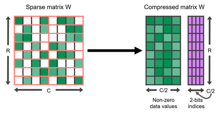
Source figure: NVIDIA, “Accelerating Inference with Sparsity Using the NVIDIA Ampere Architecture and TensorRT,” Figure 1, retrieved 2026-08-12. The figure anchors the conceptual values-plus-location split. It is not a byte-level dump of the current PyTorch or cuSPARSELt ABI, and its hardware-performance claims are not imported by this use.

0x04F A Teaching Pack Is Not A Hardware Pack

A backend-independent reference representation can retain values and logical positions:

def logical_pack_2of4(weight, selected_mask):
    validate_nm(weight, selected_mask, n_keep=2, group_size=4)

    groups = weight.reshape(weight.shape[0], -1, 4)
    masks = selected_mask.reshape(weight.shape[0], -1, 4)

    # Human-auditable representation, not cuSPARSELt/PyTorch physical bytes.
    values = groups[masks].reshape(weight.shape[0], -1, 2)
    positions = nonzero_positions_per_group(masks)  # [..., 2], each in [0, 3]
    return values, positions


def logical_decode_2of4(values, positions, original_shape):
    groups = zeros((*values.shape[:-1], 4), dtype=values.dtype)
    groups.scatter_(dim=-1, index=positions, src=values)
    return groups.reshape(original_shape)

This is suitable for parity tests and format explanation. It is not suitable as a production ABI:

• two integer positions per group would spend more bits than the fixed 4-bit metadata budget;
• a kernel may pack several group codes into one metadata word;
• values can be interleaved or swizzled by tile and lane;
• transpose and major-order choices alter physical traversal;
• backend versions can change packing while preserving logical semantics.

The converter should keep both a reference decoder and a backend compressor. Parity is checked against the reference; execution uses only the packed object accepted by the target kernel.

0x04G PyTorch Exposes A Narrow Semi-Structured Tensor Contract

As of the current PyTorch 2.13 documentation snapshot, semi-structured sparse tensors are a prototype CUDA-only tensor subclass. The documented conversion requires a contiguous 2D CUDA tensor and currently lists:

Weight dtype	Documented shape multiple for both dimensions	Pattern	Logical compression fraction
FP16	64	2:4	$9/16$
BF16	64	2:4	$9/16$
INT8	128	2:4	$10/16$

This table is a versioned API snapshot, not a hardware law. PyTorch exposes CUTLASS- and cuSPARSELt-backed subclasses with backend-specific packed state. The stable documentation lists matrix multiplication, addmm/linear, and transpose-related operations; arbitrary dense operators are not implied.

The user-facing table and one backend implementation are also different evidence surfaces. The pinned PyTorch v2.13.0 source validates CUDA, rank, contiguity, dtype, and backend-specific minimum shapes before dispatching to either a CUTLASS or cuSPARSELt subclass. Its cuSPARSELt subclass stores retained values and metadata in one packed tensor, while its CUTLASS subclass keeps packed values and metadata separately. Those implementation details constrain that exact source revision; they must not be generalized into one timeless semi-structured ABI.

A minimal inference conversion should separate semantic validation, conversion, parity, and timing:

from torch.sparse import to_sparse_semi_structured

@torch.no_grad()
def prepare_sparse_linear(linear, selected_mask, example_inputs):
    W_dense_pruned = linear.weight.detach().contiguous().cuda()
    validate_nm(W_dense_pruned, selected_mask.cuda(), 2, 4)

    W_sparse = to_sparse_semi_structured(W_dense_pruned)

    for x in example_inputs:
        dense_y = torch.nn.functional.linear(x, W_dense_pruned, linear.bias)
        sparse_y = torch.nn.functional.linear(x, W_sparse, linear.bias)
        assert_close(sparse_y, dense_y, contract_for(x.dtype))

    return W_sparse

The comparison target is W_dense_pruned, not the original dense model. That isolates representation and kernel parity from pruning quality. Original-model quality is a separate evaluation.

Conversion must happen outside the steady-state request path. The returned subclass should also be tested through the exact graph/compiler path used in deployment: eager support does not prove that an export, compiler, fusion, or distributed wrapper preserves the sparse operator.

0x04H cuSPARSELt Makes Preparation And Execution Separate Phases

The cuSPARSELt documentation snapshot retrieved for this loop identifies version 0.9.1. Because the stable URL moves, the evidence bundle records the resolved bytes and SHA-256 rather than pretending the alias is immutable. The current workflow exposes the sparse runtime contract more directly:

initialize handle
    -> declare structured and dense matrix descriptors
    -> declare op(A), op(B), layouts, dtypes, compute, epilogue
    -> create algorithm selection and matmul plan
    -> prune or accept a custom-pruned matrix
    -> run the library's pruning-validity check
    -> query compressed size and compress the sparse operand
    -> query/allocate workspace
    -> optionally search/tune an algorithm
    -> repeatedly execute matmul with new dense inputs

The distinction between prune and compress is essential. Pruning writes zeros into a dense-shape tensor. Compression creates the physical operand read by sparse matrix-multiply kernels.

A deployment wrapper should preserve the plan inputs in provenance:

SparseMatmulSignature(
    library="cuSPARSELt",
    library_version=runtime_version(),
    device_capability=current_sm(),
    logical_shape=(M_out, N_out, K_reduce),
    sparse_operand="A",
    op_a="T",
    op_b="N",
    order_a="row",
    order_b="row",
    input_dtype="fp16",
    compute_dtype="fp32",
    alignment_bytes=16,
    epilogue="bias",
    algorithm_id=selected_algorithm,
    workspace_bytes=workspace_size,
)

Do not copy those illustrative fields as universal cuSPARSELt constraints. Current library versions support multiple layouts, dtypes, compute modes, and SM generations. The executable signature must come from the descriptors and plan actually created by the installed version.

Direct cuSPARSELt invocation differs from a graph builder: if plan creation, validation, compression, or execution fails, the call has not produced a sparse result. There is no justification for silently timing an unrelated dense call under the same label.

The pinned CUDALibrarySamples matmul_example.cpp makes the order concrete: descriptor and plan creation precede prune/check and compression; optional algorithm search precedes workspace allocation and repeated matmul. The Loop 4 oracle records that source trace but does not compile or execute it.

0x04I TensorRT Separates Eligibility From Tactic Selection

TensorRT creates a second decision boundary. Its current documentation states that matrix-multiply constant weights are sparse-eligible when every four-element vector on the $K$ reduction axis has at least two zeros. The builder must also enable sparse weights and a supported precision path.

Eligibility only adds sparse tactics to the candidate set. TensorRT profiles or otherwise selects tactics for the deployed shape, and a dense tactic may be faster. Verbose build logs distinguish:

eligible sparse layers:
    pattern and graph constraints passed

layers using sparse tactics:
    builder actually selected a sparse implementation

An audit should fail if it records only the first list:

def audit_tensorrt_sparse_build(build_log, expected_layers):
    eligible = parse_sparse_eligible_layers(build_log)
    selected = parse_sparse_selected_layers(build_log)

    assert expected_layers <= eligible
    missing_sparse_tactic = expected_layers - selected
    return {
        "eligible": sorted(eligible),
        "selected_sparse": sorted(selected),
        "dense_fallback": sorted(missing_sparse_tactic),
    }

Polygraphy can inspect whether ONNX weights satisfy the structural pattern. It cannot by itself prove which tactic a later engine build selects or whether that engine improves the target workload.

0x04J The Arithmetic Ceiling Is Not The Latency Result

For $T$ input rows, $d_{in}=K$, and $d_{out}=N_o$, a dense linear layer has the usual approximate arithmetic ledger

$$F_{dense}\approx 2TN_oK.$$

An idealized N:M sparse multiply performs useful value multiplications for only the selected fraction:

$$F_{selected} \approx 2TN_oK\frac{N_{keep}}{M}.$$

For 2:4, this is half the dense multiply-add count. Sparse Tensor Core throughput is often reported in effective dense operations, which credits the skipped zero work. That convention is useful for comparing hardware capability but must not be inserted as twice as many physical nonzero multiplications in a software FLOP ledger.

A sparse operator also reads:

• compressed values and pattern metadata;
• the dense activation operand;
• output tiles and any bias/epilogue state;
• descriptors or workspace amortized by the runtime;
• possible padding and layout-conversion buffers.

A bounded model is

$$T_{sparse} \gtrsim \max \left( \frac{B_X+B_{W,values}+B_{W,meta}+B_Y}{BW_{effective}}, \frac{F_{selected}}{P_{sparse}} \right) +T_{decode/meta} +T_{launch} +T_{conversion/amortized}.$$

The compressed weight saving matters more when weight traffic is a meaningful share of the operation. Small matrices, skinny decode shapes, low occupancy, unsupported fusions, conversion in the hot path, and metadata handling can erase the arithmetic advantage.

At model level, let $f$ be the fraction of baseline latency spent in operators that are both eligible and actually dispatched sparsely. Let $S_{op}$ be their measured speedup and $o$ be new overhead normalized by baseline latency:

$$S_{end} = \frac{1} {(1-f)+f/S_{op}+o}.$$

For $f=0.70$, $S_{op}=1.5$, and $o=0.03$:

$$S_{end} \approx \frac{1}{0.30+0.70/1.5+0.03} \approx 1.26.$$

That teaching example explains why a nominal 2x sparse arithmetic capability can become a much smaller end-to-end improvement. It is not a benchmark claim.

0x04K Runtime Proof Needs A Parity Ladder And Workload Shapes

A valid experiment has at least four distinct objects:

1. original dense model, used for quality comparison;
2. N:M-pruned weights in ordinary dense storage;
3. the same pruned values decoded from or executed through the compressed representation;
4. the deployed graph and selected kernel/tactic.

Those objects induce a stricter evidence ladder:

State	Minimum evidence	Loop 4 synthetic fixture
local pattern valid	every declared row/K group has exactly two selected slots and no value outside them	proved
logical pack reversible	retained values plus logical pattern ranks decode to the same dense-pruned tensor	proved
backend artifact created	official converter returns the target backend representation and recorded bytes	not executed
operator eligible	exact dtype, shape, orientation, device, graph, and version contract passes	not claimed
sparse tactic selected	plan, algorithm, or engine-build evidence names the sparse implementation	not claimed
sparse operator observed	profiler trace identifies that implementation in the deployed path	not claimed
speedup measured	synchronized paired workload evidence beats the same pruned values run densely	not claimed

This ordering is not ceremonial. Later states consume earlier artifacts but do not follow from them logically. In particular, TensorRT eligibility can be true while tactic selection is false, and tactic selection can be true while end-to-end speedup is false.

The first comparison measures pruning error. The second proves representation parity. The third proves integration. Timing only object 1 against object 3 confounds quality, arithmetic, layout, and potentially dtype.

@torch.no_grad()
def prove_sparse_linear(candidate, workload_cases):
    W0 = candidate.original_dense_weight
    Wp = candidate.pruned_dense_weight
    Ws = candidate.packed_sparse_weight

    validate_nm(Wp, candidate.selected_mask, 2, 4)
    assert packed_nbytes(Ws) == candidate.manifest.packed_nbytes

    records = []
    for case in workload_cases:
        x = case.make_input()  # e.g. prefill tokens or active decode rows

        y_original = linear(x, W0)
        y_pruned_dense = linear(x, Wp)
        y_sparse = linear(x, Ws)

        assert_close(y_sparse, y_pruned_dense, case.numeric_contract)

        dense_profile = profile_synced(lambda: linear(x, Wp), case)
        sparse_profile = profile_synced(lambda: linear(x, Ws), case)

        records.append({
            "case": case.name,
            "pruning_error": error(y_original, y_pruned_dense),
            "representation_error": error(y_pruned_dense, y_sparse),
            "dense_pruned_ms": dense_profile.latency_ms,
            "sparse_ms": sparse_profile.latency_ms,
            "selected_kernel": sparse_profile.kernel_names,
            "workspace_bytes": sparse_profile.workspace_bytes,
        })
    return records

profile_synced must include warmup, device synchronization or CUDA events, enough repetitions, dispersion statistics, and the same stream/graph/fusion conditions. Preparation, compression, engine build, and algorithm search should be reported separately from steady state.

Transformer workload cases must include the real linear shapes:

prefill:
    T = batch * prompt tokens after packing
    large activation matrix, potentially throughput-oriented

decode:
    T = active sequences scheduled in this step
    can be small or dynamic, often latency- and launch-sensitive

tensor parallel:
    local N_o and K after sharding
    collective overlap can hide or expose local GEMM changes

A speedup measured on one large square GEMM does not establish decode latency. Conversely, a sparse kernel that loses at tiny $T$ can still improve high-load prefill throughput. The result belongs to the workload tuple, not the word “2:4.”

0x04L Semi-Structured Sparsity Is One Point In A Format Design Space

Artifact	Pattern freedom	Location state	Typical execution implication
dense tensor with zeros	arbitrary values may be zero	none beyond dense positions	ordinary dense GEMM still issues zero work
COO/CSR unstructured	arbitrary nonzeros	coordinates or row pointers plus indices	flexible, but metadata and irregular access are expensive at moderate density
block sparse	selected dense blocks	block coordinates	regular work inside blocks; quality depends on block constraint
N:M semi-structured	fixed local nonzero budget	compact fixed-pattern metadata	specialized sparse MMA path with strict dtype/shape/operator rules
smaller dense matrix	whole rows/columns physically removed	changed shapes/configuration	ordinary dense kernels on less work; owned by Loops 5-6

For FP16 at 50% density, generic CSR with 32-bit column indices already spends 2 bytes for each retained value and 4 bytes for its column index, before row pointers. That is about 3 bytes per original matrix position, larger than the 2-byte dense tensor. The 2:4 representation avoids that failure by replacing arbitrary coordinates with a tiny fixed-pattern code. Its compression comes from reduced mask entropy, not from zeros alone.

0x04M N:M And Sparse Runtime Failure Lab

Failure	Silent cause	Observable consequence	Repair
interpret prunen=1, prunem=4 as “keep one of four”	API counts removed entries, article counts retained entries	exported density is 75% instead of 25%, or vice versa	name n_keep and n_prune separately
apply one global 50% threshold	global density mistaken for local structure	some groups contain 3-4 nonzeros and fail validation	project independently inside every row/K group
group along output rows	stored matrix axes confused with logical reduction $K$	zero count looks right but kernel grouping is wrong	bind groups to logical operator coordinates
transpose after pruning without updating descriptor	physical orientation changes	packer interprets different groups	record transpose/order and validate decoded coordinates
split a K group across tensor-parallel shards	shard boundary is not divisible by $M$	local packers see incomplete groups	align K offsets/lengths or change placement
allow unstable ties	equal scores select device-dependent positions	artifact hashes differ across runs	define stable secondary ordering
mask gradients but keep old momentum	optimizer state remains nonzero in deleted slots	zeros regrow after recovery	mask parameter and same-shaped optimizer state
merge LoRA after N:M projection	dense delta writes into pruned locations	local pattern becomes invalid	merge before final projection or reproject and reevaluate
serialize dense zeros and call them compressed	no values/metadata conversion occurred	checkpoint size and dense GEMM remain unchanged	run target backend compressor and record packed bytes
hand-write a 3-bit pattern code for a 4-bit ABI	information lower bound confused with hardware encoding	decoder/kernel reads wrong positions	use official compressor and version its layout
time to_sparse_semi_structured inside forward	one-time conversion placed in hot path	sparse request is slower	convert at load/build time and time separately
compare sparse weight against original dense weight only	pruning error mixed with representation error	kernel parity cannot be isolated	compare sparse output with the same dense-pruned values
prove TensorRT eligibility only	candidate set mistaken for chosen tactic	engine may execute dense kernels	parse verbose selected-tactic evidence
benchmark only a large square GEMM	deployment uses skinny or dynamic Transformer shapes	paper speedup does not reproduce	benchmark prefill/decode and each local shard shape
report effective sparse TOPS as physical FLOPs	skipped zero work counted as executed work	compute ledger is doubled	state throughput convention and selected-value work separately

0x04N Loop Boundary

Loop 4 has now followed the complete semi-structured path:

score or reconstruction state
    -> row-local top-N_keep projection on logical K groups

fixed pattern
    -> optional mask-preserving recovery
    -> revalidation after merge, sharding, transpose, and dtype conversion

logical artifact
    -> retained values + compact pattern metadata
    -> reference decode parity

physical artifact
    -> backend descriptors, compression, workspace, and algorithm/tactic

runtime proof
    -> same pruned values through dense and sparse paths
    -> selected sparse kernel evidence
    -> prefill/decode measurements and end-to-end attribution

This closes scalar sparse execution. It does not answer which attention heads or MLP channels can be removed, because those transformations change tensor shapes and dependency graphs rather than packing scalar positions. Loop 5 owns Q/K/V/O head-slice closure and gated-MLP channel surgery.

0x05 Structural Surgery Removes Coupled Head And MLP Slices

An N:M mask preserves every matrix shape. Head and MLP-channel pruning make a different promise: delete a complete computational term, remove every parameter slice that produces or consumes that term, and export smaller dense matrices. Ordinary dense kernels can then execute the reduced shapes without decoding sparse metadata. That apparent simplicity hides a dependency problem.

A head is not one row in one tensor. In classic MHA it occupies matching output blocks in Q, K, and V, then an input block in the output projection. A SwiGLU channel occupies one output row in both gate_proj and up_proj, then one input column in down_proj. Biases, per-channel quantization state, adapters, optimizer tensors, packed layouts, tensor-parallel shards, configuration, and cache metadata can carry the same axis.

The owner question for this loop is:

How does a low-importance gate become a dependency-closed tensor slice, a reloadable smaller checkpoint, and a measured dense execution path without accidentally changing residual width or GQA sharing semantics?

Loop 5 keeps the residual stream at width $d$. It owns the internal attention width $H_qd_h$, the persistent KV width $H_{kv}d_h$, and the MLP intermediate width $d_{ff}$. Removing residual channels would propagate through embeddings, normalization, every block, and the LM head; that global transformation remains the Loop 6 boundary.

The replayable evidence for this loop deliberately stops below a framework or model reproduction. It executes one deterministic row-major fixture with classic MHA, equal-group GQA, an irregular query-only GQA alternative, and SwiGLU. The oracle proves logical-to-stored index maps, gate-zero versus sliced forward parity, packed-layout maps, parameter and KV ledgers, target-TP ownership, and architecture-manifest round trips. It does not claim that a paper checkpoint was pruned, that a production loader accepted heterogeneous shapes, that a GPU kernel ran, or that latency or quality improved.

@dataclass(frozen=True)
class StructuralSurgeryManifest:
    residual_width: int
    head_dim: int
    original_q_heads: int
    original_kv_heads: int
    kept_q_heads_original: tuple[int, ...]
    kept_kv_heads_original: tuple[int, ...]
    q_to_kv_new: tuple[int, ...]
    attention_layout: str
    original_mlp_width: int
    kept_mlp_channels_original: tuple[int, ...]
    mlp_layout: str
    target_tp: int
    kv_placement: str

This manifest distinguishes original coordinates from compacted coordinates. The distinction matters whenever a surviving noncontiguous head owns ALiBi, QK normalization, cache state, quantization metadata, or an adapter slice.

0x05A A Gate Defines The Unit Before A Score Ranks It

For one attention layer, split the output projection into row-vector algebraic blocks $W_O^{(h)}\in\mathbb R^{d_h\times d}$ and write

$$Y = \operatorname{Concat}(A_1,\ldots,A_H)W_O = \sum_{h=1}^{H} A_hW_O^{(h)},$$

where $A_h\in\mathbb R^{T\times d_h}$ is the value-mixed output of head $h$. Insert one scalar gate per head:

$$Y(g) = \sum_{h=1}^{H}g_hA_hW_O^{(h)}.$$

Now $g_h=0$ has a precise counterfactual: the entire projected contribution of head $h$ is absent. With upstream gradient $G_Y=\partial L/\partial Y$, the chain rule gives

$$\frac{\partial L}{\partial g_h} = \left\langle G_Y, A_hW_O^{(h)} \right\rangle_F.$$

Equivalently, if the gate is applied directly to $A_h$, this is the inner product of $A_h$ with its own backpropagated gradient. Michel et al. estimate head importance as

$$I_h^{Michel} = \mathbb E_{x\sim\mathcal D} \left[ \left| \frac{\partial L(x)}{\partial g_h} \right| \right].$$

The absolute value is inside the data expectation. Moving it outside would let positive and negative samples cancel. The paper computes the score with forward/backward passes, normalizes within each layer by the layer score $\ell_2$ norm, and uses iterative greedy removal. This is a post-training local sensitivity proxy, not proof that jointly pruning several low-score heads has the sum of their individual effects.

Voita et al. instead learn stochastic head gates with a differentiable relaxation of an $L_0$ penalty. In schematic form:

$$\min_{\theta,\phi} \mathbb E_{z\sim q_\phi} \left[L(\theta,z)\right] + \lambda\sum_h\Pr_\phi(z_h\ne0).$$

That objective lets task loss and sparsity pressure co-adapt. A binary exported gate still has to be converted into physical tensor slices; expected gate sparsity alone does not shrink a checkpoint or select a faster kernel.

The source-series figure below records the empirical observation that specialized positional, syntactic, and rare-token heads tended to survive longer in the studied translation encoders. It should not be read as a universal taxonomy for every decoder-only LLM.

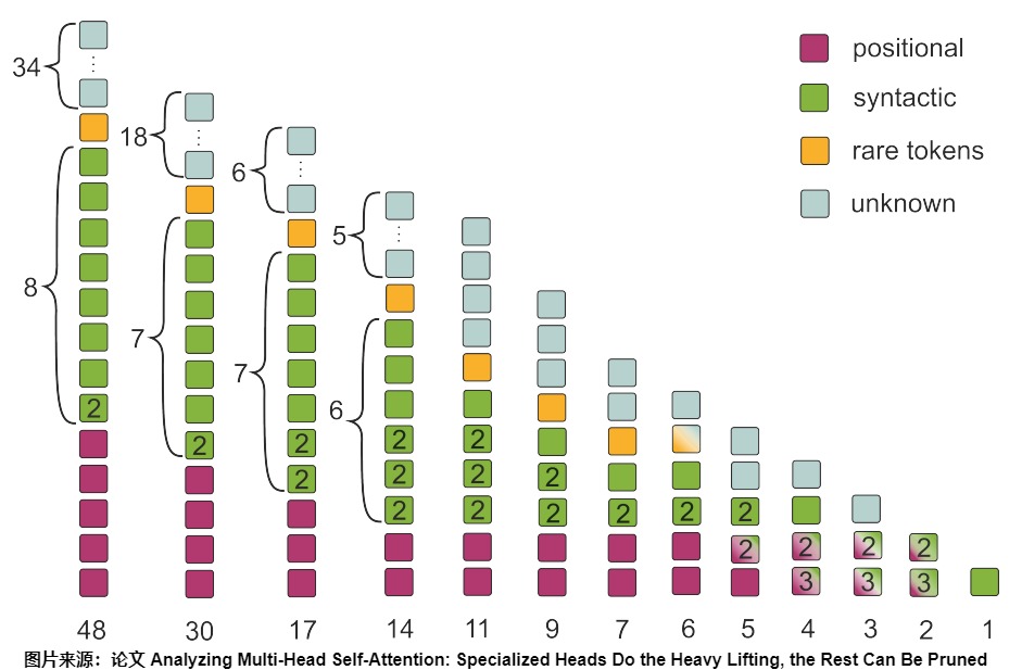
Source-local reconstruction from A12, based on Voita et al., Figure 8. The empirical result is architecture-, task-, and training-run-scoped.

The next source-series figure makes the training object explicit: a gate multiplies each head output and the optimization penalizes nonzero gates.

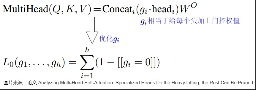
Source-local reconstruction from A12, based on Voita et al. The blue annotation explains that each head receives a gate.

Four common selectors answer different questions:

Selector	Signal	Extra work	What it does not prove
direct ablation	measured $L(g_h=0)-L(g_h=1)$	one or more evaluations per candidate	joint subset quality
Michel Taylor gate	$\mathbb E	\partial L/\partial g_h	$
learned $L_0$ gate	task loss plus expected active-unit penalty	sparsity-aware training	exact exported budget without projection
grouped weight criterion	aggregate magnitude/Taylor terms over all coupled slices	weights only or calibration backward	equivalence between different group sizes/costs

Scores are meaningful only after the unit is defined. Ranking one Q row, one head, one KV-sharing group, and one MLP channel in a single raw list silently compares objects with different parameter, FLOP, cache, and quality costs. A cost-aware target can instead solve a constrained selection problem:

$$\min_{z\in\{0,1\}^{U}} \widehat{\Delta L}(z) \quad\text{subject to}\quad \sum_{u=1}^{U}z_uc_u\le B,$$

where $c_u$ must name the target resource: parameters, bytes, projection MACs, prefill attention MACs, KV bytes, or measured latency. These budgets are not interchangeable.

0x05B A Zero Head Gate Has An Exact Smaller-Dense Counterpart

Use row-vector algebra for classic MHA:

$$W_Q,W_K,W_V\in\mathbb R^{d\times Hd_h}, \qquad W_O\in\mathbb R^{Hd_h\times d}.$$

Let $\mathcal H$ be the kept head set and expand it into a kept channel index:

$$\mathcal I(\mathcal H) = \bigcup_{h\in\mathcal H} \{hd_h,hd_h+1,\ldots,(h+1)d_h-1\}.$$

The structurally reduced matrices are

$$W_Q'=W_Q[:,\mathcal I], \quad W_K'=W_K[:,\mathcal I], \quad W_V'=W_V[:,\mathcal I], \quad W_O'=W_O[\mathcal I,:].$$

Under PyTorch nn.Linear, weights are stored as [out_features,in_features]. The same operation therefore becomes:

q_proj.weight: keep rows I
k_proj.weight: keep rows I
v_proj.weight: keep rows I
o_proj.weight: keep columns I

q/k/v bias:    keep entries I
o_proj bias:   unchanged, because residual output width d is unchanged

This is not merely shape bookkeeping. Partitioning $W_O$ by head proves

$$\sum_{h\in\mathcal H}A_hW_O^{(h)} = \operatorname{Concat}_{h\in\mathcal H}(A_h) W_O[\mathcal I,:].$$

Therefore, in deterministic evaluation mode, the physically sliced module must match the original module with deleted head gates fixed to zero. That gate-zeroed dense path is the representation-parity oracle. Comparing only to the original unpruned module mixes intentional pruning error with export bugs.

The Q/K/V slices are needed to stop computing the deleted head. Slicing only the corresponding input columns of $W_O$ produces the same gated function but still computes the deleted Q/K/V projections, score matrix, softmax, and value mix. Conversely, deleting Q/K/V blocks without slicing $W_O$ changes the concat width and makes the consumer invalid.

For classic MHA, one full head without projection biases owns

$$P_{head}^{MHA} = 3dd_h+dd_h = 4dd_h$$

weights. For $d=4096$ and $d_h=128$:

Q row block: 4096 * 128 =   524,288 weights
K row block: 4096 * 128 =   524,288 weights
V row block: 4096 * 128 =   524,288 weights
O col block: 4096 * 128 =   524,288 weights
total:                     2,097,152 weights = 4 MiB at FP16

For self-attention over $T$ token rows, the removed head’s projection work is $4Tdd_h$ MACs. Its two core attention products contribute approximately $2T^2d_h$ MACs in prefill: one $QK^T$ and one probability-value product. The exact kernel ledger also includes softmax, masking, RoPE, reads/writes, launch, and fusion boundaries.

In classic MHA the persistent KV payload for one removed head is

$$M_{KV,head} = 2Td_hb$$

bytes per layer and request, where $b$ is bytes per cached element. With $d_h=128$ and FP16, that is 512 bytes per cached token per layer. This cache saving does not carry over to query-only pruning in GQA or MQA.

The LLM-Pruner paper frames the same problem as discovery of coupled groups. Its Figure 2 separates MLP intermediate groups, attention-head groups, and a global residual-channel group. Loop 5 owns the first two; Loop 6 owns the globally propagating channel-wise group on the right.

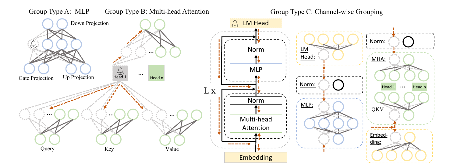
Source: Ma, Fang, and Wang, LLM-Pruner, Figure 2. Cropped from the official paper for legibility.

0x05C Slice Modules By Stored Axis, Then Prove The Function

A reference implementation should name output and input slicing separately. It should also preserve device, dtype, bias policy, and requires_grad rather than constructing default CPU/FP32 modules by accident:

def copy_linear_out(linear, keep_out):
    keep_out = as_index(keep_out, device=linear.weight.device)
    new = nn.Linear(
        in_features=linear.in_features,
        out_features=len(keep_out),
        bias=linear.bias is not None,
        device=linear.weight.device,
        dtype=linear.weight.dtype,
    )
    with torch.no_grad():
        new.weight.copy_(linear.weight.index_select(0, keep_out))
        if linear.bias is not None:
            new.bias.copy_(linear.bias.index_select(0, keep_out))
    new.weight.requires_grad_(linear.weight.requires_grad)
    if new.bias is not None:
        new.bias.requires_grad_(linear.bias.requires_grad)
    return new


def copy_linear_in(linear, keep_in):
    keep_in = as_index(keep_in, device=linear.weight.device)
    new = nn.Linear(
        in_features=len(keep_in),
        out_features=linear.out_features,
        bias=linear.bias is not None,
        device=linear.weight.device,
        dtype=linear.weight.dtype,
    )
    with torch.no_grad():
        new.weight.copy_(linear.weight.index_select(1, keep_in))
        if linear.bias is not None:
            new.bias.copy_(linear.bias)  # output axis was not reduced
    new.weight.requires_grad_(linear.weight.requires_grad)
    if new.bias is not None:
        new.bias.requires_grad_(linear.bias.requires_grad)
    return new

Classic separate-projection MHA surgery is then explicit:

def expand_head_indices(keep_heads, head_dim):
    return torch.tensor([
        h * head_dim + offset
        for h in keep_heads
        for offset in range(head_dim)
    ])


def prune_classic_mha_heads(attn, keep_heads):
    assert is_classic_mha(attn)
    keep = expand_head_indices(keep_heads, attn.head_dim)

    attn.q_proj = copy_linear_out(attn.q_proj, keep)
    attn.k_proj = copy_linear_out(attn.k_proj, keep)
    attn.v_proj = copy_linear_out(attn.v_proj, keep)
    attn.o_proj = copy_linear_in(attn.o_proj, keep)

    attn.num_heads = len(keep_heads)
    attn.num_key_value_heads = len(keep_heads)
    attn.inner_dim = len(keep_heads) * attn.head_dim
    return attn

This mirrors the dependency direction in the historical Hugging Face BERT prune_heads implementation: Q/K/V are sliced on linear output, while the attention output dense layer is sliced on linear input. That implementation is useful evidence for the tensor operation, not a universal modern API contract; generic head pruning was removed from the Transformers v5 surface.

At the pinned Transformers v4.0.1 commit, BertAttention.prune_heads first maps original head ids around already_pruned_heads, then applies dim=0 to Q/K/V and dim=1 to the output dense layer before updating both num_attention_heads and all_head_size. The helper constructs new linear modules, copies the selected weights and the axis-appropriate bias, and does not preserve an optimizer object. Those details support this slice direction; they do not establish a GQA, packed-QKV, TP, cache, or exact-resume contract.

Before mutating the model, capture the gate-zeroed oracle. After surgery, test the same input, mask, positions, dtype, and evaluation mode:

with torch.no_grad():
    y_masked = dense_attn(x, head_gate=keep_mask, use_cache=False)
    y_small = sliced_attn(x, use_cache=False)

torch.testing.assert_close(y_small, y_masked, rtol=rtol, atol=atol)

Then repeat with prefill and one-token decode cache paths. A no-cache parity test does not validate KV head count, cache append shape, cache reorder, or position-dependent kernels.

0x05D GQA Makes Query Heads And KV Groups Different Pruning Units

Grouped-query attention has

$$H_q>H_{kv}, \qquad G=\frac{H_q}{H_{kv}},$$

under the common equal contiguous-group mapping. Every group of $G$ query heads reads one shared K/V head. MQA is the limiting case $H_{kv}=1$.

Removing one query head requires only:

q_proj: remove one output head block
o_proj: remove the matching input head block
k_proj, v_proj: unchanged
KV cache: unchanged

The parameter saving is $2dd_h$, half of a classic MHA head, and there is no persistent KV-cache saving because the shared K/V head remains. The resulting query-to-KV map may become irregular: after deleting one member, an equal group no longer contains exactly $G$ contiguous query heads. A runtime that derives the map from integer division cannot represent that arbitrary subset merely by changing num_attention_heads.

There are three different export choices:

1. Prune a complete GQA group. Remove $G$ Q blocks, their $G$ O input blocks, and the one shared K and V block. Equal grouping survives.
2. Prune query heads only. Preserve K/V and store an explicit surviving query-to-KV map. This needs a model and kernel that accept that map.
3. Repartition or merge. Change which queries share each KV head, then recover quality. This is an architecture conversion, not simple deletion.

A complete equal GQA group owns

$$P_{group}^{GQA} = Gdd_h+2dd_h+Gdd_h = 2(G+1)dd_h$$

weights across Q, K/V, and O. With $d=4096$, $d_h=128$, and $G=4$, this is 5,242,880 weights, or 10 MiB at FP16. It also removes one K/V head from the cache. In MQA, the sole shared K/V head cannot be removed while any query head still needs attention, so query-head pruning saves projection and attention work but not cache width.

def prune_equal_gqa_groups(attn, keep_kv_groups):
    group = attn.num_heads // attn.num_key_value_heads
    assert attn.num_heads % attn.num_key_value_heads == 0

    keep_q_heads = [
        kv * group + local
        for kv in keep_kv_groups
        for local in range(group)
    ]
    q_idx = expand_head_indices(keep_q_heads, attn.head_dim)
    kv_idx = expand_head_indices(keep_kv_groups, attn.head_dim)

    attn.q_proj = copy_linear_out(attn.q_proj, q_idx)
    attn.k_proj = copy_linear_out(attn.k_proj, kv_idx)
    attn.v_proj = copy_linear_out(attn.v_proj, kv_idx)
    attn.o_proj = copy_linear_in(attn.o_proj, q_idx)

    attn.num_heads = len(keep_q_heads)
    attn.num_key_value_heads = len(keep_kv_groups)
    assert attn.num_heads // attn.num_key_value_heads == group
    return attn

Full-head deletion keeps $d_h$ constant, so the within-head Q/K dot-product and RoPE pair layout remain unchanged. Reducing $d_h$ is a different operation: it slices coordinates inside every surviving head, changes RoPE dimensions and possibly scaling, alters attention kernel shapes, and must coordinate Q, K, V, and O at sub-head granularity. Loop 5 records it as an alternative, not as head pruning.

0x05E Packed Projections And Tensor Parallelism Change The Index Map

The equations above assume separate Q, K, V parameters whose output rows are head-major. Production checkpoints may store any of these layouts:

contiguous packed MHA:
    [Q_all_heads | K_all_heads | V_all_heads]

head-interleaved MHA:
    [Q_0 | K_0 | V_0 | Q_1 | K_1 | V_1 | ...]

group-packed GQA:
    [Q_group_0 | K_0 | V_0 | Q_group_1 | K_1 | V_1 | ...]

separate projections:
    q_proj, k_proj, v_proj

The same logical head set maps to different physical rows in each format. A converter must read the model implementation or an explicit layout descriptor; inferring pack order from a tensor shape is impossible because several layouts have the same number of elements.

@dataclass(frozen=True)
class AttentionLayout:
    kind: str                  # separate, qkv_contiguous, head_interleaved, ...
    num_q_heads: int
    num_kv_heads: int
    head_dim: int
    q_to_kv: tuple[int, ...]
    tensor_parallel_size: int


def physical_rows_for_heads(layout, keep_q, keep_kv):
    if layout.kind == "separate":
        return {
            "q": expand_head_indices(keep_q, layout.head_dim),
            "k": expand_head_indices(keep_kv, layout.head_dim),
            "v": expand_head_indices(keep_kv, layout.head_dim),
        }
    if layout.kind == "qkv_contiguous":
        return contiguous_qkv_row_map(layout, keep_q, keep_kv)
    if layout.kind == "group_interleaved":
        return grouped_qkv_row_map(layout, keep_q, keep_kv)
    raise UnsupportedLayout(layout.kind)

Per-head QK normalization, head-specific scaling, ALiBi slopes, relative-bias tables, attention sinks, or other head-axis parameters must follow the same kept-head map. Full-head pruning leaves RMSNorm/LayerNorm on the residual stream unchanged, but a head-local norm is not residual normalization and cannot be ignored.

Tensor parallelism adds ownership constraints. A common placement uses column-parallel Q/K/V projections, whose output channels are partitioned, and a row-parallel O projection, whose input channels use the matching partition. Gated MLPs similarly place gate/up output channels and down input channels on the same rank. The structural keep set must therefore be converted from global indices to each rank’s local indices on all coupled tensors.

The safest export order is:

unsharded logical checkpoint
    -> choose dependency-closed units
    -> slice full tensors
    -> update architecture manifest
    -> repartition the new shapes for target TP degree

Slicing already-sharded tensors is valid only when the converter knows global offsets and can rebalance ownership. Otherwise one rank may retain more heads or MLP channels than another, collective split sizes can disagree, and a locally valid checkpoint can deadlock or fail at all-reduce/all-gather.

Runtime-friendly targets often round kept counts so local dimensions remain aligned:

$$H_q'\bmod TP=0, \qquad H_{kv}'\ \text{is representable by the target KV placement}, \qquad d_{ff}'\bmod (TP\cdot a)=0,$$

where $a$ is a kernel alignment measured in local channels. These are target runtime constraints, not universal mathematical requirements. LLM-Pruner’s official Llama-3 path, for example, groups K projection output channels in consecutive blocks of head_dim, prunes with dependency groups, then derives each layer’s num_heads and num_key_value_heads from the resulting projection shapes. The code and README also expose the practical consequence of heterogeneous per-layer widths: a conventional scalar config and ordinary from_pretrained() path may no longer reconstruct the model.

That statement is version-specific. At the pinned LLM-Pruner commit, the earlier hf_prune.py block-wise path roots attention groups at q_proj, groups consecutive head_dim rows, and refreshes only num_heads. The later llama3.py path roots them at k_proj and refreshes both query- and KV-head counts from projection shapes. The shared dependency engine propagates root indices through graph mappings and rejects groups that would remove every channel. Neither path is promoted here as a universal irregular-GQA exporter; the fixture therefore treats complete equal GQA groups and query-only irregular maps as different artifact contracts.

0x05F One SwiGLU Channel Is A Three-Slice Computational Term

For a gated LLaMA-style MLP with row-vector input $x\in\mathbb R^d$:

$$g=xW_g, \qquad u=xW_u, \qquad a=\operatorname{SiLU}(g)\odot u, \qquad y=aW_d,$$

with

$$W_g,W_u\in\mathbb R^{d\times d_{ff}}, \qquad W_d\in\mathbb R^{d_{ff}\times d}.$$

Write the two input-projection columns as $w_{g,j}$ and $w_{u,j}$ and row $j$ of $W_d$ as $w_{d,j}^{T}$. The MLP is a sum of intermediate-channel terms:

$$y = \sum_{j=1}^{d_{ff}} \operatorname{SiLU}(xw_{g,j}) (xw_{u,j}) w_{d,j}^{T}.$$

Insert a gate $z_j$ on the product:

$$y(z) = \sum_{j=1}^{d_{ff}} z_j \operatorname{SiLU}(xw_{g,j}) (xw_{u,j}) w_{d,j}^{T}.$$

This expansion proves the dependency group. If channel $j$ is deleted, its gate-projection column, up-projection column, and down-projection row must all disappear in algebraic notation. In stored PyTorch nn.Linear weights, that is:

gate_proj.weight [d_ff,d]: keep output rows J
up_proj.weight   [d_ff,d]: keep output rows J
down_proj.weight [d,d_ff]: keep input columns J

gate/up bias [d_ff]:       keep entries J, if present
down bias [d]:             unchanged

The gate-gradient analogue is

$$\frac{\partial L}{\partial z_j} = \left\langle G_y, a_jw_{d,j}^{T} \right\rangle,$$

where $a_j=\operatorname{SiLU}(xw_{g,j})(xw_{u,j})$. A grouped Taylor score can estimate this directly with a channel gate or aggregate weight-gradient terms over all three coupled slices. Those estimators are not necessarily identical: placing one shared gate after the elementwise product measures the signed joint contribution of the complete channel, while summing absolute scalar $|w\,\partial L/\partial w|$ terms discards cancellation within the group.

A classic two-matrix GELU/ReLU FFN owns only the input-projection output row and the output-projection input column. Its per-channel parameter saving is $2d$. SwiGLU owns three slices and saves

$$P_{channel}^{SwiGLU}=3d$$

weights per removed intermediate channel, excluding optional bias. With $d=4096$, one channel is 12,288 weights, or 24 KiB at FP16. Removing 1,024 channels from a $d_{ff}=11{,}008$ MLP produces $d_{ff}'=9{,}984$ and removes 12,582,912 weights, exactly 24 MiB of FP16 parameter payload. It also removes $3Td\cdot1024$ projection MACs for $T$ token rows, before kernel overhead.

The width 9,984 may be mathematically valid yet poorly aligned for a target kernel or tensor-parallel degree. A deployment target may instead remove a nearby number of channels in aligned groups. That changes the realized budget and must be reflected in the quality evaluation rather than reported as the unrounded score target.

0x05G MLP Surgery Uses One Keep Set Across Every Branch

def prune_swiglu_channels(mlp, keep_channels):
    keep = as_index(keep_channels, device=mlp.gate_proj.weight.device)

    assert mlp.gate_proj.out_features == mlp.up_proj.out_features
    assert mlp.gate_proj.out_features == mlp.down_proj.in_features

    mlp.gate_proj = copy_linear_out(mlp.gate_proj, keep)
    mlp.up_proj = copy_linear_out(mlp.up_proj, keep)
    mlp.down_proj = copy_linear_in(mlp.down_proj, keep)
    mlp.intermediate_size = len(keep)
    return mlp

For a packed gate_up_proj with stored output shape [2*d_ff,d], the keep set must be translated through pack order. Under a simple contiguous [gate_all | up_all] layout:

packed_keep = torch.cat([keep, keep + old_intermediate_size])
mlp.gate_up_proj = copy_linear_out(mlp.gate_up_proj, packed_keep)
mlp.down_proj = copy_linear_in(mlp.down_proj, keep)

An interleaved [gate_0,up_0,gate_1,up_1,...] layout needs a different map. As with packed QKV, shape alone does not reveal the order.

The dependency closure also extends into training and compression state:

State attached to the channel axis	Required action
Adam moments or master weights	slice with the same stored axis if training continues
LoRA on gate/up output	slice LoRA $B$ output rows; $A$ input side is unchanged
LoRA on down input	slice LoRA $A$ input columns; $B$ output side is unchanged
per-output quantization scale on gate/up	slice scale entries or requantize
per-input/group quantization state on down	regenerate groups after slicing
tensor-parallel checkpoint shards	repartition global keep set and rewrite shard metadata

Merging adapters before surgery followed by slicing the merged dense weights is usually easier to audit. If runtime adapter switching must survive, every adapter needs the same architecture manifest and compatible sliced shapes.

0x05H Selection, Surgery, And Recovery Are Different Phases

A robust structural-pruning pipeline separates at least five states:

1. dense trainable model
2. model with explicit head/channel gates for scoring or sparsity training
3. frozen discrete keep sets under an exact architecture/resource budget
4. physically sliced smaller-dense model
5. recovered and deployment-converted model

Collapsing them creates reproducibility gaps. A paper may report gate sparsity from state 2, parameter count from state 4, and quality after state 5. The article or release manifest must say which state produced each number.

Three practical schedules have different tradeoffs:

Post-training score, then surgery

calibration forward/backward
    -> fixed Taylor/magnitude/ablation scores
    -> exact keep-set projection
    -> physical slice
    -> optional recovery

This is inexpensive and close to Michel-style sensitivity pruning, but scores are local to the dense checkpoint. Large one-shot removals can invalidate the ranking because surviving units have not adapted.

Iterative prune and recover

score -> remove a bounded fraction -> short recovery
      -> rescore the changed model -> repeat

This tracks interactions better but increases training and evaluation cost. The ranking, optimizer, calibration data, random seed, and per-step budget all become part of the experiment contract.

Joint stochastic gates

train weights and relaxed gates under task + resource penalty
    -> anneal or harden gates
    -> exact budget projection
    -> physical slice
    -> recovery / final validation

This lets the model redistribute function while sparsity develops, as in Voita-style $L_0$ gates. A penalty coefficient does not guarantee a requested integer head count or aligned d_ff; a final constrained projection remains necessary.

LLM-Pruner instantiates a related discovery-estimation-recovery pipeline. It discovers dependent groups, estimates group importance using magnitude or Taylor-style terms on limited public samples, removes groups, then applies LoRA recovery. Its official implementation exposes block-wise attention/MLP, channel-wise residual-width, and layer-wise modes. Its published quality, timing, and data-volume results are source-reported examples, not defaults for other models or pruning ratios.

Recovery can use full fine-tuning, LoRA, distillation, or a combination:

$$L_{recover} = \lambda_{task}L_{task} + \lambda_{logit}L_{KD} + \lambda_{hidden}L_{hidden}.$$

The student is already structurally smaller. Hidden-state losses are easy at the residual boundary because Loop 5 keeps width $d$ unchanged; matching the deleted intermediate head/channel tensors themselves is neither possible nor necessary. M6.10 owns the full distillation target and divergence design.

After the keep set is frozen, removed units should not reappear. Gate training can retain relaxed gate parameters, but the final sliced model has no deleted slots to regrow. If surgery occurs mid-optimization, recreate or explicitly slice optimizer state; attaching an old dense optimizer to new parameter objects is invalid.

0x05I The Architecture Manifest Is Part Of The Artifact

A state dictionary alone does not fully describe a pruned model. The loader must know how each changed tensor maps to logical heads and channels:

{
  "layer": 12,
  "attention": {
    "layout": "separate_q_k_v",
    "head_dim": 128,
    "kept_query_heads_original": [0, 1, 4, 5, 8, 9, 12, 13],
    "kept_kv_heads_original": [0, 1],
    "q_to_kv_new": [0, 0, 0, 0, 1, 1, 1, 1],
    "num_attention_heads": 8,
    "num_key_value_heads": 2
  },
  "mlp": {
    "layout": "separate_gate_up_down",
    "intermediate_size": 9984,
    "kept_channel_hash": "sha256:..."
  }
}

Uniform pruning can update ordinary scalar configuration fields when every layer shares the same new num_attention_heads, num_key_value_heads, and intermediate_size. Heterogeneous pruning needs per-layer metadata or custom module construction. Saving a Python module object, as one reference LLM-Pruner path does for heterogeneous shapes, can preserve structure for one environment but is not a portable substitute for a versioned architecture and state-dict format.

Migration must cover:

model config and per-layer overrides
state-dict tensor shapes and safetensors shard index
packed QKV / gate-up order
original-to-new head and channel maps
RoPE and head-local parameter shapes
KV-cache head count and query-to-KV map
tensor-parallel ownership and collective split sizes
quantization scales, groups, and excluded modules
adapter shapes and adapter registry compatibility
optimizer/scheduler state if training resumes
artifact schema version and source checkpoint hash

A clean release test constructs the pruned architecture from the manifest, loads the state dict with no missing or unexpected parameters, saves it again, reloads in a fresh process, and reproduces logits and cache shapes. Passing an in-memory forward before serialization is insufficient.

The Loop 5 fixture makes the bookkeeping concrete without borrowing a paper result:

Fixture branch	Original geometry	Kept original units	Exact structural consequence
classic MHA	$d=4$, $H=3$, $d_h=2$	heads $\{0,2\}$	96 to 64 weights; 12 to 8 cached K/V scalars per token
equal GQA	$d=4$, $H_q=4$, $H_{kv}=2$, $G=2$	KV group $\{1\}$ and query heads $\{2,3\}$	96 to 48 weights; 8 to 4 cached K/V scalars per token
query-only GQA	same source	query heads $\{0,2,3\}$, both KV heads	16 weights removed; K/V cache unchanged; equal integer grouping no longer represents the map
SwiGLU	$d=4$, $d_{ff}=6$	channels $\{0,2,4,5\}$	72 to 48 weights through one shared three-slice keep set

For every branch, the oracle compares the physically reduced computation to the source computation with exactly the deleted terms gated to zero. It also maps the same keep sets through contiguous and interleaved QKV/gate-up layouts. Those equalities prove conversion semantics only; they do not prove that the removed terms were a good quality choice.

0x05J Prove Four Different Things Before Claiming Speed

Structural pruning needs a layered validation ladder.

1. Dependency and shape proof

assert q_proj.out_features == num_q_heads * head_dim
assert k_proj.out_features == num_kv_heads * head_dim
assert v_proj.out_features == num_kv_heads * head_dim
assert o_proj.in_features == num_q_heads * value_head_dim

assert gate_proj.out_features == intermediate_size
assert up_proj.out_features == intermediate_size
assert down_proj.in_features == intermediate_size

Also validate biases, per-head parameters, pack order, TP divisibility, and the query-to-KV map.

2. Representation parity

Compare the sliced model against the same dense model with deleted head/channel gates fixed to zero. Run block-level and full-model checks, then prefill and incremental decode with cache. This isolates conversion correctness from intentional quality loss.

3. Quality and recovery proof

Compare the original model, gate-zeroed model, freshly sliced model, and recovered model on calibration-held-out loss and task suites. Keep source domains separate from evaluation domains. A low calibration loss increase can hide degraded rare capabilities or long-context behavior.

4. Runtime proof

Record actual parameter bytes, local GEMM shapes, kernel names, workspace, prefill latency, decode latency, throughput, KV bytes, and end-to-end serving metrics. Smaller dense dimensions remove arithmetic, but latency can fail to improve when:

• dimensions lose favorable tile alignment;
• per-layer heterogeneous shapes prevent graph reuse or fusion;
• the attention kernel pads to a supported head count;
• TP imbalance or extra collectives replace local work;
• decode remains dominated by unrelated weight or KV traffic;
• launch, sampling, communication, or non-pruned layers dominate.

For MHA with kept fraction $r_H=H'/H$, the idealized projection and core attention arithmetic scale approximately with $r_H$ when $d_h$ remains fixed. For GQA query-only pruning, Q/O and query-head attention work scale with $r_{H_q}$, while K/V projection and KV cache do not. For SwiGLU with kept fraction $r_F=d_{ff}'/d_{ff}$, its three large projection matrices scale with $r_F$. End-to-end speed still follows the measured eligible fraction:

$$S_{end} = \frac{1} {(1-f)+f/S_{struct}+o},$$

where $f$ is baseline time in successfully reduced operators and $o$ includes conversion-induced overhead. Parameter reduction percentage is not a valid substitute for $f$.

0x05K The Main Variants Differ In Selection And Export, Not Just Score Name

Method or system	Unit	Selection/training	Physical export lesson	Evidence boundary
Michel et al.	individual attention head	post-training expected absolute gate gradient; iterative pruning	paper studies head removal and speed potential; converter details are architecture-specific	NMT and BERT experiments in the paper
Voita et al.	attention head	stochastic gates with differentiable $L_0$ pressure	learned zero gates still require structural export for smaller dense tensors	NMT models and identified head roles
historical HF BERT pruning	BERT head	caller supplies head indices	Q/K/V output rows plus output-dense input columns; updates local head metadata	versioned BERT implementation, not current universal API
DepGraph	graph-derived coupled group	dependency discovery plus chosen importance rule	structural coupling can be discovered through graph dependencies	evaluated architectures in the paper
LLM-Pruner	LLM MLP/head groups, residual channel groups, or layers	dependency discovery, grouped magnitude/Taylor estimation, optional LoRA recovery	heterogeneity and view/concat index mapping complicate portable loading	source-reported LLaMA/Vicuna/ChatGLM and later code support
this article’s exporter	explicit MHA/GQA/SwiGLU unit	selector is pluggable; keep set is projected under runtime constraints	gate-zero parity, versioned manifest, fresh-process reload, and runtime proof are mandatory	rewrite audit framework

Head merging, MHA-to-GQA conversion, and low-rank factorization can reduce similar matrices but are not deletion. Merging changes the surviving function and usually needs alignment or retraining. N:M preserves matrix shapes. Residual-width slicing propagates globally. Layer pruning removes whole ordered blocks. Keeping these artifacts separate makes both quality and runtime claims auditable.

0x05L Structural Surgery Failure Lab

Failure	Silent cause	Observable consequence	Repair
zero one head gate and report a smaller model	functional ablation mistaken for physical export	unchanged checkpoint and dense kernels	slice every producer/consumer axis and recount bytes
slice Q/K/V but not O	concat consumer retains old input width	shape error or wrong channel interpretation	slice matching O input columns
slice only O input columns	deleted head is hidden after compute	little or no attention-core saving	also remove Q/K/V blocks when execution should shrink
prune one GQA query head and decrement KV heads	query and shared-KV units conflated	wrong cache shape and group map	keep KV or prune a complete sharing group
preserve counts but not original head map	surviving noncontiguous heads renumbered silently	wrong per-head bias, scale, or cache assignment	serialize original-to-new maps
infer packed QKV order from shape	several layouts have equal shape	Q rows can become K/V rows	use implementation-specific layout descriptor
prune gate rows but not up rows	SwiGLU branches disagree	elementwise product shape error or semantic mismatch	one keep set for gate, up, and down
prune both axes of down_proj	intermediate width confused with residual width	downstream residual addition fails	Loop 5 changes down input only
leave old optimizer moments attached	parameter objects and state shapes changed	load error or corrupt recovery	recreate or explicitly migrate state
apply dense LoRA after slicing	adapter dimensions reference deleted axes	merge/load failure	merge before surgery or slice every adapter consistently
update global config for heterogeneous layers	scalar field cannot describe per-layer shapes	fresh load constructs wrong modules	use per-layer manifest/custom architecture or uniform target
keep arbitrary head/channel counts	mathematical shape accepted but target kernel/TP is not	padding, fallback, imbalance, or compile failure	project budget onto runtime-supported aligned counts
compare sliced output only to original dense	pruning damage and conversion error mixed	parity bug can hide inside expected quality loss	compare first to gate-zeroed dense oracle
validate prefill without cached decode	cache metadata and append path untested	generation fails after first token	run multi-step decode and cache reorder tests
count removed weights as latency reduction	removed operators are not baseline bottleneck	negligible end-to-end gain	profile eligible time and measure target workload
cite one paper’s removable-head ratio as a rule	redundancy is checkpoint/task dependent	aggressive quality regression	rescore and evaluate the actual model and domains

0x05M Loop Boundary

Loop 5 has now followed complete internal-width surgery:

define unit with an explicit gate
    -> estimate or learn importance under declared data and reduction order
    -> project onto exact quality/resource/runtime constraints

dependency closure
    -> MHA: Q/K/V output blocks + O input block
    -> GQA: distinguish query-head and shared-KV-group units
    -> SwiGLU: gate/up output rows + down input columns

physical export
    -> map logical units through packed layout and TP ownership
    -> migrate biases, head-local state, quantization, adapters, and config
    -> serialize a versioned per-layer architecture manifest

proof
    -> gate-zeroed dense parity
    -> fresh-process save/load parity
    -> prefill and cached-decode quality
    -> actual smaller-dense kernels and workload latency

The residual stream has remained width $d$ throughout. Loop 6 starts where that assumption is removed. It owns globally coupled residual-channel deletion, SliceGPT’s computational-invariance framing, embedding/norm/LM-head closure, and the difference between local intermediate-width surgery and whole-model dense matrix slicing.

The article-local Loop 5 bundle freezes the exact paper and implementation loci, the synthetic surgery manifest, all formula and visual identities, and one-field failure cases. Its claim ceiling remains below framework execution, paper reproduction, GPU/runtime measurement, recovery, deployment, and final publication closure.

0x06 Residual-Width Slicing Changes Every Block Boundary

Loop 5 removed complete terms inside attention and MLP branches while the residual stream kept width $d$. Residual-width pruning removes coordinates from the state that joins those branches. The dependency group is therefore no longer local to one module. It starts at every embedding that creates residual state, crosses every shortcut and normalization boundary, touches the input and output side of every residual branch, and ends at every consumer of the final state.

The owner question is:

How can a pretrained Transformer compute in a lower-dimensional residual space when its useful directions are not aligned with the checkpoint’s coordinate axes, and how do we separate an exact change of basis from the lossy deletion that follows it?

The replayable evidence for this loop uses one deterministic row-major D=4 fixture. It proves full-width rotation parity, physically sliced forward parity against an independently lifted projected-coordinate reference, non-parity against the unsliced model after truncation, original-dimension RMS normalization, global tensor-axis closure, rectangular shortcut shapes, endpoint-dependent parameter ledgers, unchanged K/V payload, and slicing- manifest round trips. It does not run the SliceGPT framework, prune a paper checkpoint, reproduce paper quality, execute a GPU kernel, measure speed, run recovery, or validate deployment.

@dataclass(frozen=True)
class ResidualWidthSlicingManifest:
    source_checkpoint_sha256: str
    model_family: str
    original_hidden_size: int
    norm_reference_dimension: int
    boundary_bases: tuple[str, ...]
    boundary_dimensions: tuple[int, ...]
    attention_input_dimensions: tuple[int, ...]
    attention_output_dimensions: tuple[int, ...]
    mlp_input_dimensions: tuple[int, ...]
    mlp_output_dimensions: tuple[int, ...]
    shortcut_shapes: tuple[tuple[int, int], ...]
    do_slice_head: bool
    head_dimension: int
    endpoint_policy: str
    calibration_manifest_sha256: str
    state_dict_sha256: str

The bases are executable coordinate state, not interchangeable metadata. The widths determine stored tensor shapes; norm_reference_dimension preserves the normalization denominator; and do_slice_head determines whether the final boundary remains narrow or expands back to the original LM-head width.

SliceGPT provides the main worked system for this loop. It rotates each block-boundary signal into a data-derived basis, keeps a leading subspace, and replaces affected matrices with smaller dense matrices. Its paper calls this post-training sparsification, but its executable artifact is not a zero mask or a CSR/N:M tensor. It is a custom Transformer whose residual dimensions, shortcut operators, and dense matrix shapes have changed.

The paper’s first figure makes that artifact distinction visible. Unstructured and 2:4 pruning retain a dense activation width and encode zeros in the weight. Slicing removes a complete activation coordinate and the corresponding matrix axis after a rotation.

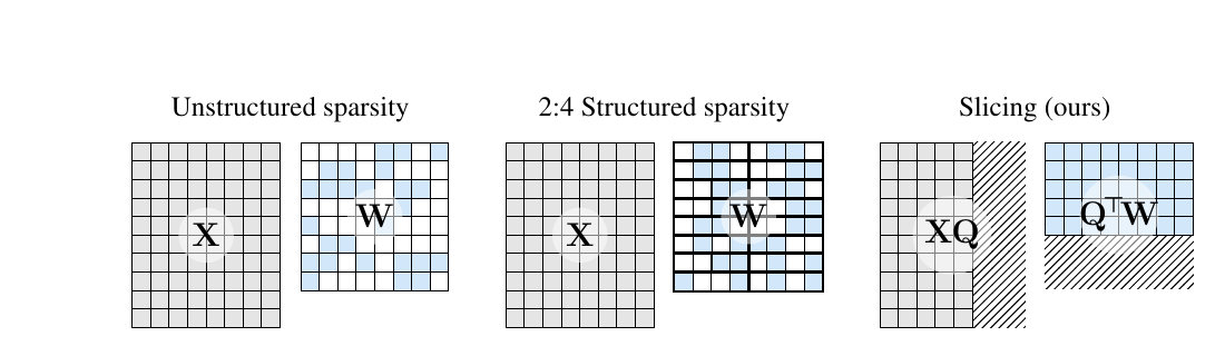
Source: Ashkboos et al., SliceGPT, Figure 1. Cropped from the official ICLR 2024 paper. The hatched regions are deleted, not stored as sparse zeros.

0x06A A Residual Coordinate Is A Whole-Graph Unit

Consider a LLaMA-style sequential decoder block:

$$h_\ell = x_\ell + \operatorname{Attn}_\ell(\operatorname{Norm}_{a,\ell}(x_\ell)),$$ $$x_{\ell+1} = h_\ell + \operatorname{MLP}_\ell(\operatorname{Norm}_{m,\ell}(h_\ell)).$$

The additions require both operands at each boundary to use the same shape and the same coordinate interpretation. Deleting coordinate $j$ from $x_\ell$ therefore propagates through every producer and consumer of that state.

For one uniform direct-coordinate keep set $J$, dependency closure includes:

token / learned-position / type embeddings:
    keep residual output columns J

attention branch:
    Q/K/V projections keep residual input columns J
    O projection keeps residual output rows J

gated MLP branch:
    gate/up projections keep residual input columns J
    down projection keeps residual output rows J

normalization and residual-local state:
    transform or slice learned affine state consistently
    keep both operands of every residual add in the same basis

output boundary:
    final normalization follows the new state contract
    LM head keeps residual input columns J, unless an explicit final bridge
    expands into a different head space

In PyTorch storage, input axes are linear-weight columns and output axes are linear-weight rows. This is the opposite visual direction for some matrices from row-vector algebra. A valid exporter names both conventions.

This global coupling explains why the channel-wise group on the right side of the LLM-Pruner figure in 0x05B reaches from embedding to LM head. A single ordinary mask must be shared across all residual boundaries because identity shortcuts cannot add two different coordinate systems. SliceGPT relaxes that single-mask restriction by inserting explicit basis-change operators into the shortcuts.

Local MLP-channel pruning and residual-width pruning are therefore different:

Transformation	Width changed	Coupled axes	Attention/KV consequence
Loop 5 SwiGLU channel deletion	$d_{ff}$	gate/up output and down input	none
Loop 5 head deletion	$H_qd_h$ and optionally $H_{kv}d_h$	Q/K/V output and O input	may reduce KV only when a K/V unit is removed
Loop 6 residual slicing	boundary state $d$	embeddings, branch inputs/outputs, shortcuts, norms, head boundary	does not by itself change $H_q$, $H_{kv}$, or $d_h$

0x06B Orthogonal Rotation Is Exact Before Any Coordinate Is Deleted

First remove the learned affine scale from the notation and define a bare row-wise RMS normalization with fixed reference dimension $D$:

$$\operatorname{RMSN}_D(x) = \frac{x} {\sqrt{\frac{1}{D}\lVert x\rVert_2^2+\epsilon}}.$$

Let $Q\in\mathbb R^{D\times D}$ be orthogonal:

$$Q^TQ=QQ^T=I.$$

Orthogonality preserves the row norm:

$$\lVert xQ\rVert_2^2 = xQQ^Tx^T = xx^T = \lVert x\rVert_2^2.$$

The denominator is therefore unchanged and

$$\operatorname{RMSN}_D(XQ) = \operatorname{RMSN}_D(X)Q,$$

or equivalently

$$\operatorname{RMSN}_D(XQ)Q^T = \operatorname{RMSN}_D(X).$$

This commutation relation is the computational invariance. It is exact up to floating-point evaluation order. It does not say that deleting coordinates is exact.

For row-vector algebra, a branch with input linear $W_{in}$ and output linear $W_{out}$ can compute in the rotated residual basis $\widetilde X=XQ$ by using

$$\widetilde W_{in}=Q^TW_{in}, \qquad \widetilde W_{out}=W_{out}Q.$$

The internal branch preactivation is unchanged:

$$\widetilde X\widetilde W_{in} = XQQ^TW_{in} = XW_{in},$$

while the branch output is expressed in the new residual basis:

$$F(\widetilde X\widetilde W_{in})\widetilde W_{out} = F(XW_{in})W_{out}Q.$$

The residual sum then obeys

$$XQ+F(XW_{in})W_{out}Q = \left(X+F(XW_{in})W_{out}\right)Q.$$

The same basis must reach the boundaries:

$$\widetilde E=EQ, \qquad \widetilde W_{LM}=Q^TW_{LM}$$

in row-vector algebra, where $E\in\mathbb R^{V\times D}$ and $W_{LM}\in\mathbb R^{D\times V}$. Then $XQ\widetilde W_{LM}=XW_{LM}$ and the logits remain unchanged.

Biases follow the axis they inhabit. An output bias in residual coordinates rotates with the output; an internal input-linear bias is unchanged because the internal preactivation is unchanged. In PyTorch storage, the official code implements the same algebra as:

# nn.Linear stores [out_features, in_features]
input_linear.weight  = input_linear.weight @ Q
output_linear.weight = Q.T @ output_linear.weight
output_linear.bias   = Q.T @ output_linear.bias

embedding.weight     = embedding.weight @ Q
lm_head.weight       = lm_head.weight @ Q

The last line is consistent because lm_head.weight is stored as $[V,D]$ and is transposed by the linear operation at runtime.

0x06C Learned Normalization State Does Not Commute For Free

A standard LLaMA RMSNorm is not only $\operatorname{RMSN}_D$. It applies a learned elementwise scale $\gamma$:

$$\operatorname{RMSNorm}_\gamma(x) = \operatorname{RMSN}_D(x)\operatorname{diag}(\gamma).$$

For a general dense $Q$,

$$\operatorname{diag}(\gamma)Q \ne Q\operatorname{diag}(\gamma).$$

Leaving the learned scale in place and rotating only neighboring weights would therefore break the claimed invariance. SliceGPT folds each norm’s scale into the subsequent input linears, clones the LM-head weight when it had shared storage with the embedding, and replaces affine normalization modules with an unparameterized RMSN.

LayerNorm adds mean subtraction and often an affine shift. Define

$$M = I-\frac{1}{D}\mathbf1\mathbf1^T.$$

Then $XM$ subtracts each row mean. The paper rewrites LayerNorm-connected models into an RMSNorm-connected form by absorbing:

LayerNorm scale gamma:
    into the following branch input matrices

mean-subtraction matrix M:
    into preceding branch output matrices and embeddings

final normalization scale:
    into the LM head

LayerNorm bias / downstream affine terms:
    into compatible adjacent biases where the architecture permits

This is an architecture conversion with an exact pre-slice parity obligation, not permission to replace arbitrary LayerNorms with RMSNorms. Post-LN ordering, parallel branches, fused biases, tied weights, and model-specific norm implementations all affect the legal fusion. The official repository requires a ModelAdapter and LayerAdapter for each supported family rather than assuming one universal rewrite.

There is another subtle implementation contract. The official replacement module stores the original hidden size as mean_dim and computes

variance = x.pow(2).sum(-1, keepdim=True) / original_hidden_size

even after $x$ has only $d'<D$ coordinates. Replacing it with an ordinary RMSNorm(d'), which divides by $d'$, changes the scale by approximately $\sqrt{D/d'}$ when epsilon is negligible. The normalization denominator is part of the sliced artifact.

0x06D Different Boundary Bases Turn Identity Shortcuts Into Matrices

One global orthogonal $Q$ can rotate the entire residual stream without adding runtime operations: every identity shortcut still maps $XQ$ to $XQ$. But the activation covariance can have a different principal basis at each boundary. SliceGPT therefore uses $Q_a$ before a residual branch and $Q_b$ after it.

The branch output can be rotated into $Q_b$, but the residual arrives in basis $Q_a$. Before addition it must be mapped by

$$R_{a\rightarrow b} = Q_a^TQ_b,$$

because

$$(XQ_a)R_{a\rightarrow b} = XQ_aQ_a^TQ_b = XQ_b.$$

After slicing, let $D_a\in\mathbb R^{D\times d_a}$ and $D_b\in\mathbb R^{D\times d_b}$ select retained coordinates in the two rotated bases. The executable shortcut is rectangular:

$$S_{a\rightarrow b} = D_a^TQ_a^TQ_bD_b \in \mathbb R^{d_a\times d_b}.$$

It maps a stored state $Z_a=XQ_aD_a$ into the next retained basis. Before truncation, $R$ is an exact change of basis. After truncation, $S$ cannot reconstruct components that $D_a$ already discarded. It is part of the lossy compressed graph, not a proof that the sliced graph equals the original.

A sequential LLaMA block has two residual additions and therefore two such shortcut matrices: one around attention and one around the MLP. A parallel attention/MLP block can share one output boundary and uses a different adapter path. The official CompressedLlamaDecoderLayer makes this runtime state explicit:

rotated_residual = residual @ self.attn_shortcut_Q
hidden_states = rotated_residual + attention_output

rotated_residual = hidden_states @ self.mlp_shortcut_Q
hidden_states = rotated_residual + mlp_output

These are dense matrix multiplications. They cannot generally be folded into a branch weight because the shortcut bypasses the branch nonlinearity.

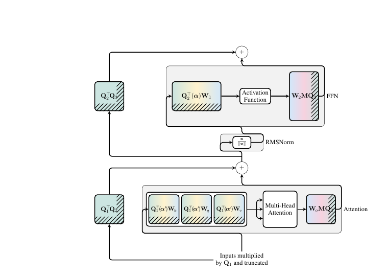
Source: Ashkboos et al., SliceGPT, Figure 4. Cropped from the official paper. Hatched matrix regions are removed; $Q_{\ell-1}^TQ_\ell$ remains executable shortcut work.

0x06E PCA Selects Directions, Not Original Semantic Channels

Directly deleting low-norm coordinate columns assumes that useful residual directions already align with the checkpoint axes. SliceGPT instead collects boundary activations $X_{\ell,i}$ from calibration sequences and forms

$$C_\ell = \sum_i X_{\ell,i}^TX_{\ell,i}.$$

Let

$$C_\ell = Q_\ell\Lambda_\ell Q_\ell^T, \qquad \lambda_1\ge\lambda_2\ge\cdots\ge\lambda_D.$$

Keeping the first $d'$ eigenvectors gives

$$Z=XQD, \qquad \widehat X=Z D^TQ^T,$$

where $D=[e_1,\ldots,e_{d'}]$. For the stated squared reconstruction objective, the retained subspace is optimal and the calibration reconstruction error is

$$\lVert X-\widehat X\rVert_F^2 = \sum_{j=d'+1}^{D}\lambda_j.$$

That theorem concerns reconstruction of the sampled boundary activations. It does not guarantee language-model loss, downstream accuracy, rare-domain behavior, or long-context quality.

A two-dimensional toy example shows why rotation matters. Suppose

$$C = \begin{bmatrix} 5&4\\ 4&5 \end{bmatrix}.$$

Its eigenvectors are $q_1=(1,1)/\sqrt2$ and $q_2=(1,-1)/\sqrt2$ with eigenvalues $9$ and $1$. Keeping one principal coordinate preserves $90\%$ of the sampled squared energy and incurs reconstruction error $1$. Deleting either original coordinate instead discards an axis with diagonal energy $5$. PCA first aligns the high-energy diagonal direction with a coordinate that can be physically kept.

The official implementation is specifically an uncentered Gram/eigensystem calculation, despite using the name PCA:

H = sum_over_batches_and_tokens(X.T @ X)
H += 0.01 * mean(diag(H)) * I
eigvals, Q = torch.linalg.eigh(H.double())
Q = Q[:, argsort(eigvals, descending=True)]

Padding rows are zeroed before accumulation. Adding a scalar multiple of the identity leaves exact eigenvectors unchanged while improving numerical conditioning; finite-precision and repeated-eigenvalue behavior can still vary. The paper reports that eigenvector precision affected large-model accuracy and used double precision for its main PCA calculation. That is a source-reported numerical finding, not a universal requirement for every eigensolver and model.

Calibration choices are part of the method. The paper studies sample count and sequence length and uses larger settings in its main experiments. The current official experiment script defaults to 128 samples and sequence length 2,048. Those are code defaults, not proof that 128 samples cover the deployment distribution.

The Loop 6 fixture makes the exactness boundary numeric. It uses three distinct orthogonal 4 x 4 bases and keeps three coordinates at each compressed boundary. The full-width transformed network matches its original reference. The sliced graph matches the same graph with each discarded projector written explicitly, but intentionally differs from the full-width reference:

Contract	Stored widths	Expected relation
full rotation	4 -> 4 -> 4	transformed logits equal original logits
fully narrow slicing	3 -> 3 -> 3	physical tensors equal projected-coordinate reference; original parity is false
expanded-head slicing	3 -> 3 -> 4	final shortcut is rectangular and the original-width head remains; original parity is still false
wrong sliced norm	mean_dim=3 instead of original D=4	logits differ from the valid sliced graph

For the fixture’s two-branch, vocabulary-six ledger, the unsliced core has 88 weights. The fully narrow artifact has 66 core weights plus 18 shortcut weights, for 84 total. The expanded-head artifact has 74 core weights plus 21 shortcut weights, for 95 total. The tiny expanded case is deliberately larger than its baseline: reducing a width is not sufficient evidence of reducing the serialized model once bridges and endpoint policy are counted.

0x06F Rotation And Slicing Must Advance Through The Actual Model

Each later basis is estimated from activations produced by the already transformed path. A practical sequential pass is:

inputs = capture_first_layer_inputs(calibration_batches)

# Embedding -> first attention boundary
_, Q = pca_gram(inputs, attention_masks)
rotate_and_slice_embeddings(Q, d_embed)

for layer in layers:
    layer.attn_shortcut = previous_Q.T @ Q
    rotate_attention_input_columns(layer, Q)
    slice_attention_input_columns(layer, d_attn_in)

    attn_to_mlp_states = run_to_mlp_boundary(layer, inputs)
    _, Q_next = pca_gram(attn_to_mlp_states, attention_masks)
    rotate_attention_output_rows(layer, Q_next)
    slice_attention_output_rows(layer, d_attn_out)
    slice_shortcut_both_axes(layer.attn_shortcut, d_attn_in, d_attn_out)

    layer.mlp_shortcut = Q_next.T
    rotate_and_slice_mlp_inputs(layer, Q_next, d_mlp_in)

    outputs = run_complete_compressed_layer(layer, inputs)
    _, Q_out = pca_gram(outputs, attention_masks)
    rotate_and_slice_mlp_output(layer, Q_out, d_mlp_out)
    finish_rectangular_shortcut(layer.mlp_shortcut, Q_out, d_mlp_in, d_mlp_out)

    inputs = outputs
    Q = Q_out

This is a mechanism sketch, not drop-in code. The official implementation also moves layers between CPU and the selected device, updates the layer’s forward arguments, distinguishes sequential and parallel blocks, supports constant and configured per-boundary schedules, and optionally changes the orientation inside the retained subspace.

Its final_orientation="random" option right-multiplies $Q$ by an orthogonal matrix that acts only inside the retained leading block. This changes the coordinates within the same retained subspace, not which subspace survives. final_orientation="pca" leaves principal axes explicit. The choice can alter finite-precision and downstream compression behavior even though ideal subspace reconstruction is unchanged.

At the pinned Microsoft TransformerCompression commit 6b12cdee6ad51791d7c776b3a046bc408b9e77e9, the prose maps to concrete files:

File	Exact implementation contract used here
src/slicegpt/rotate.py	sequential/parallel activation propagation, Q estimation, input/output slicing, rectangular shortcut construction, optional head slicing, and PCA damping/eigendecomposition
src/slicegpt/layernorm_fusion.py	compressed-layer replacement, tied-head clone, embedding mean subtraction, affine norm fusion, and replacement by bare RMSN
src/slicegpt/modules.py	RMSN.mean_dim remains the original hidden size even when the stored last axis is narrower
src/slicegpt/slicing_scheduler.py	per-boundary dimensions are recorded; do_slice_head=False is the default and returns the final boundary to the original hidden size
src/slicegpt/model_adapter.py	compressed layers register shortcut parameters and SlicingConfig serializes every boundary dimension and endpoint policy
src/slicegpt/adapters/llama_adapter.py	LLaMA executes residual @ attn_shortcut_Q and residual @ mlp_shortcut_Q before the two additions
src/slicegpt/hf_utils.py	fresh loading constructs compressed modules, fuses norms, allocates shortcut state, restores JSON config, slices the uninitialized graph, then loads weights
experiments/run_slicegpt.py	the experiment path replaces/fuses modules, creates a constant scheduler, rotates/slices, and saves both state dictionary and JSON config

That trace is version-specific. It verifies what this repository revision does; it does not establish one universal SliceGPT ABI or prove compatibility with a newer Transformers release, tensor-parallel engine, compiler, or quantized loader.

0x06G Every Stored Axis Has A Different Slice Direction

For a sequential decoder with boundary dimensions $d_a$ before a branch and $d_b$ after it, the stored PyTorch axes are:

Parameter	Dense stored shape	Rotate	Slice	Result
token embedding	[V,D]	right by $Q_0$	columns	[V,d_0]
learned additive embedding	[N,D] or equivalent	right by $Q_0$	columns	[N,d_0]
Q/K/V weight	[d_{q/kv},D]	right by $Q_a$	input columns	[d_{q/kv},d_a]
O weight	[D,d_q]	left by $Q_b^T$	output rows	[d_b,d_q]
gate/up weight	[d_{ff},D]	right by $Q_b$	input columns	[d_{ff},d_b]
down weight	[D,d_{ff}]	left by $Q_c^T$	output rows	[d_c,d_{ff}]
shortcut	[D,D] conceptually	$Q_a^TQ_b$	rows and columns	[d_a,d_b]
LM head weight	[V,D]	right by $Q_L$	input columns when enabled	[V,d_L]

The attention inner outputs $d_q=H_qd_h$ and $d_{kv}=H_{kv}d_h$ need not equal the new residual width. Residual slicing changes the input dimension of Q/K/V and the output dimension of O. It need not delete heads or coordinates inside a head. Similarly, it changes gate/up input columns and down output rows, not the MLP intermediate width $d_{ff}$.

Two small helpers express the physical operation:

def rotate_and_slice_input(linear, Q, keep_dim):
    # stored [out, residual_in]
    W = linear.weight.double() @ Q.double()
    linear.weight = nn.Parameter(W[:, :keep_dim].to(linear.weight.dtype))
    linear.in_features = keep_dim


def rotate_and_slice_output(linear, Q, keep_dim):
    # stored [residual_out, inner]
    W = Q.double().T @ linear.weight.double()
    linear.weight = nn.Parameter(W[:keep_dim, :].to(linear.weight.dtype))
    if linear.bias is not None:
        b = Q.double().T @ linear.bias.double()
        linear.bias = nn.Parameter(b[:keep_dim].to(linear.bias.dtype))
    linear.out_features = keep_dim

These helpers are valid only after the architecture adapter has identified which linears enter and leave each residual boundary. Cross-attention, parallel residual branches, mixture-of-experts shared/routed paths, adapters, multimodal projectors, and recurrent state connectors add more consumers to the closure.

0x06H Embeddings, Tied Weights, And The Final Head Need An Explicit Policy

Every tensor added into the first residual state must use the same retained basis. Token embeddings are not enough when a model also has learned position, segment, modality, prompt, or vision-projector outputs. A state can have the right width and still use the wrong basis.

Input embedding and output head weights are often tied. Under one shared full rotation and one shared slice, both stored [V,D] tensors can transform as $W\leftarrow WQD$ and remain tied. Per-boundary SliceGPT generally uses different first and last bases, and it may choose different endpoint widths. The official fusion code clones the LM-head weight before modifying embeddings, explicitly breaking shared parameter storage so the two boundaries can evolve independently.

The current official main experiment creates ConstSlicingScheduler(new_embedding_dimension) with do_slice_head=False. The scheduler therefore keeps the final head dimension at the original hidden size: the final layer’s output path and shortcut return to that width, and the LM head is rotated but not sliced. Head slicing is supported as an option, not the default path. Consequently, the phrase “SliceGPT reduces embedding dimension” does not imply that every released/configured path slices the LM head input identically.

An artifact must declare one of these endpoint contracts:

fully narrow endpoint:
    input embedding [V,d0]
    final state [B,S,dL]
    LM head [V,dL]
    tied weights possible only if endpoint basis/width policy permits

expanded head endpoint:
    narrow internal state
    final branch/shortcut maps back to original D
    original-width LM head remains

external bridge:
    narrow Transformer state
    explicit learned/fixed bridge into a different head or projector width

The tokenizer and vocabulary axis do not change. Slicing an embedding column is not vocabulary pruning.

0x06I Residual Slicing Does Not Automatically Shrink KV Cache

Suppose GQA uses

$$d_q=H_qd_h, \qquad d_{kv}=H_{kv}d_h.$$

Residual slicing from $D$ to $d'$ changes:

q_proj: [d_q,D]   -> [d_q,d']
k_proj: [d_kv,D]  -> [d_kv,d']
v_proj: [d_kv,D]  -> [d_kv,d']
o_proj: [D,d_q]   -> [d',d_q]

The produced K/V vectors still have width $d_{kv}$. Therefore

$$M_{KV} = 2T H_{kv}d_h b$$

is unchanged unless head count or head width is also reduced. QK score and probability-value attention MACs are also unchanged because their head-space dimensions are unchanged. Residual slicing reduces Q/K/V projection input work, O projection output work, residual activation traffic, MLP residual-axis work, and possibly embeddings/head work.

This makes Loop 5 and Loop 6 complementary. A compound exporter may first choose head/KV groups and MLP channels, then rotate and slice residual widths, but the transforms do not commute blindly. The dependency map, calibration activations, quantization scales, adapters, and recovery all need to be recomputed for the chosen order.

0x06J Parameter And MAC Ledgers Must Include Shortcut Work

Ignoring biases and normalization, one LLaMA-style layer has residual-axis linear parameters

$$P_{core}(D) = 2D d_q + 2D d_{kv} + 3D d_{ff}.$$

The first two terms count Q/O and K/V; the third counts gate, up, and down. If only residual dimensions become $d'=rD$ while head and MLP inner dimensions stay fixed:

$$P_{core}(d')=rP_{core}(D).$$

For sequential blocks with two distinct sliced shortcut maps of shape $d'\times d'$, add approximately

$$P_{shortcut}=2d'^2$$

parameters and the same number of MACs per token row. Variable widths instead add $d_a d_b$ for each boundary map.

For a toy LLaMA-like layer with $D=4096$, $d_q=d_{kv}=4096$, $d_{ff}=11{,}008$, and $d'=3072$:

baseline residual-axis core:
    4 * 4096^2 + 3 * 4096 * 11008
    = 202,375,168 weights

sliced core before shortcuts:
    0.75 * baseline
    = 151,781,376 weights

two 3072 x 3072 shortcuts:
    18,874,368 weights

sliced core plus shortcuts:
    170,655,744 weights

net reduction in this ledger:
    31,719,424 weights, about 15.7%, not 25%

Embedding tables can contribute a large additional saving: $V(D-d')$ values per sliced table. A sliced LM head contributes another $V(D-d')$ unless weights remain tied or the head endpoint expands. Conversely, custom shortcut state and untied endpoint weights can add payload. The width ratio $1-d'/D$ is not the same as whole-model parameter sparsity; the official script separately measures the final parameter count for this reason.

The MAC ledger follows the same linear reductions for branch projections and adds shortcut GEMMs. It must then account for unchanged attention-core work, unchanged KV cache, normalization, RoPE, sampling, collectives, and kernel alignment. Smaller dense dimensions make ordinary dense-kernel acceleration possible, but do not guarantee it.

0x06K Uniform And Variable Schedules Trade Simplicity For Fit

The current official code supports several shape policies:

Policy	Basis	Width schedule	Shortcut consequence	Deployment consequence
one global coordinate mask	original axes	usually constant	identity shortcut survives	simplest loader; weakest alignment to each boundary distribution
one global orthogonal basis	one $Q$	constant	identity shortcut survives	no shortcut GEMM, but one basis must fit all layers
SliceGPT constant scheduler	different $Q_\ell$	common retained width internally	dense square shortcuts	regular GEMM shapes; custom compressed layer
SliceGPT configured/function scheduler	different $Q_\ell$	boundary-dependent widths	dense rectangular shortcuts	better local fit is possible; heterogeneous shapes complicate kernels and sharding
global residual-channel dependency pruning	original learned axes	selected coordinates	identity shortcut survives if one map is global	no rotation overhead; selection/recovery bears alignment burden
low-rank factorization	learned/fitted factors	factor rank per matrix	residual width may remain $D$	two GEMMs and intermediate factor activations rather than one smaller dense model

Per-layer spectrum decay does not automatically prove that heterogeneous widths are better. The SliceGPT appendix reports model-dependent results when varying slice level by layer. Width schedules need held-out quality and runtime evaluation rather than an eigenvalue-only decision.

0x06L Calibration, Recovery, And Deployment Are Separate Costs

SliceGPT is post-training in the sense that rotation and initial slicing do not require updating the base weights by gradient descent. It still needs calibration examples, layer executions, activation Gram accumulation, an eigendecomposition at each boundary, model conversion, and evaluation. The paper also studies optional recovery fine-tuning; the official repository provides a LoRA recovery path.

Keep these phases separate:

calibration and basis discovery
    -> dataset, sample count, sequence lengths, padding mask, precision

exact architecture conversion
    -> norm fusion, model adapter replacement, full rotations, parity

lossy slicing
    -> width schedule, endpoint policy, rectangular shortcuts

optional recovery
    -> task data, LoRA/full parameters, objective, optimizer, merge policy

deployment conversion
    -> dtype/quantization, sharding, compile, kernels, cache, manifest

Quantization after rotation sees different weight and activation distributions; pre-existing group scales are no longer valid. Quantizing first and then performing dense rotations generally requires dequantization or a compatible quantized transform. Tensor parallel shards must be regenerated from global sliced tensors because both residual-axis ownership and shortcut dimensions change. LoRA attached before rotation must be merged or transformed on the same axes; adding LoRA after slicing is simpler.

The paper’s throughput, GPU-count, and quality results are source-reported for its models, hardware, calibration, and evaluation setup. They demonstrate that smaller dense execution can produce real gains; they are not a portable latency multiplier for another runtime.

0x06M The Artifact Requires A Compressed Architecture, Not Just New Weights

The official pipeline performs three architectural stages:

replace_layers(model_adapter)
    -> install compressed layer classes with shortcut matrices

fuse_modules(model_adapter)
    -> absorb affine norms / mean subtraction and install bare RMSN

rotate_and_slice(model_adapter, calibration_loader, scheduler)
    -> estimate bases, rotate weights, slice axes, attach shortcut state

It saves the sliced state_dict together with a JSON SlicingConfig containing embedding, attention-input/output, MLP-input/output, and head dimensions. A loader must construct the custom compressed modules before loading that state. Merely changing a stock Hugging Face hidden_size is insufficient because:

• head-space widths can remain at their original values;
• residual widths can differ by boundary;
• shortcut matrices are new executable parameters;
• normalization uses an original-dimension denominator;
• the final head may intentionally retain original width;
• standard tied-weight and cache assumptions may no longer hold.

A release manifest should include model-family adapter version, source checkpoint hash, calibration contract, basis/scheduler policy, every boundary dimension, endpoint policy, norm conversion, shortcut shapes, original and final parameter counts, dtype, sharding, and recovery lineage.

0x06N Validation Must Stop At Each Exactness Boundary

The safest validation ladder is:

1. Norm-fusion parity

Compare the original model with the model after affine/mean folding and custom layer replacement, before rotation or slicing. Check intermediate boundaries, logits, and cached decode.

2. Full-rotation parity

Apply square $Q_\ell$ matrices and unsliced $Q_{\ell-1}^TQ_\ell$ shortcuts. Compare against the fused model. This tests orientation, stored axes, biases, parallel/sequential branch handling, and the final head.

3. Slicing quality, not parity

After applying $D_\ell$, exact equality to the dense model is no longer expected. Measure calibration reconstruction, held-out language-model loss, task suites, rare/long-context behavior, and generation. A parity assertion at this stage would be the wrong contract.

4. Fresh-process artifact proof

Reconstruct modules from the slicing config, load with no missing or unexpected state, and reproduce sliced-model logits and cache behavior. Test endpoint weight tying, generation, serialization, and multiple sequence lengths.

5. Runtime proof

Record final parameter bytes, shortcut bytes/MACs, activation width, actual GEMM shapes, selected kernels, sharding, peak memory, prefill, decode, throughput, KV bytes, and end-to-end latency. Attribute the gain to narrower dense work rather than to the nominal slicing percentage.

0x06O Residual-Width Failure Lab

Failure	Silent cause	Observable consequence	Repair
delete residual coordinate $j$ in only one layer	identity shortcuts globally couple the state	add/next-layer shape failure or coordinate drift	close the dependency graph or insert an explicit compatible bridge
call the orthogonal rotation lossy	exact basis change and truncation conflated	inability to localize conversion bugs	prove full-rotation parity before applying $D$
call PCA truncation exact	invariance theorem applied after deleting coordinates	unacknowledged quality loss	treat slicing as approximation and evaluate it
rotate linears but leave learned RMSNorm scale	diagonal affine state does not commute with dense $Q$	logits drift before slicing	fold norm state into adjacent modules and parity-test
replace sliced norm with ordinary RMSNorm(d')	denominator changes from original $D$ to $d'$	systematic activation rescaling	serialize and preserve normalization reference dimension
use different $Q$ per boundary but retain identity shortcut	residual and branch outputs use different bases	semantically invalid addition	execute $D_a^TQ_a^TQ_bD_b$ on the shortcut
omit shortcut parameters from parameter/FLOP count	bridge work treated as free	overstated compression and speed	count every square/rectangular shortcut
slice Q/K/V output rows as residual pruning	head coordinates confused with residual input	accidental head-width/head-count change	slice Q/K/V input columns; leave head outputs unless separately pruned
claim residual slicing reduces KV cache	K/V output dimension stayed fixed	cache bytes do not move	combine with explicit KV-head/width pruning if desired
rotate token embeddings but not learned position/type embeddings	additive sources use different bases	wrong initial residual state	transform every residual-state producer
preserve tied storage across different endpoint bases	input and output endpoints require incompatible transforms	one boundary silently becomes wrong	enforce shared endpoint policy or untie explicitly
report width sparsity as parameter sparsity	$1-d'/D$ ignores embeddings, head, shortcuts, and unsliced axes	misleading artifact size	recount the serialized model
compute bases from padded tokens	padding distribution enters $X^TX$	unstable or domain-specific components	mask padded rows before accumulation
use one calibration domain and claim universal subspace quality	principal directions are data-dependent	rare/domain performance regression	declare data contract and evaluate held-out domains
reuse quantization scales after rotation	basis change changes tensor distributions and groups	poor quality or invalid group metadata	recalibrate/requantize after final slicing
mutate already-sharded tensors without global maps	residual axes cross TP ownership	collective mismatch or rank imbalance	transform globally, then repartition and validate collectives
load sliced weights into a stock model	custom shortcuts and dimensions are absent	missing keys, shape errors, or wrong forward	construct versioned compressed modules from manifest first
infer speed from the paper’s GPU result	source setup treated as universal	deployment misses target	benchmark the actual runtime, hardware, batch, and sequence mix

0x06P Loop Boundary

Loop 6 has now followed the residual coordinate from source to sink:

global dependency closure
    -> all embeddings and residual-state producers
    -> Q/K/V and gate/up residual input axes
    -> O and down residual output axes
    -> norm state, shortcuts, final norm, and output boundary

exact conversion
    -> fold noncommuting normalization state
    -> rotate each boundary with orthogonal Q
    -> prove full-width logits and cache parity

lossy compression
    -> estimate uncentered activation Gram matrices
    -> retain a PCA subspace with explicit D
    -> slice linears and rectangular shortcut matrices

artifact and runtime proof
    -> custom compressed layer + slicing manifest
    -> fresh-process reload and held-out quality
    -> count shortcut work and unchanged KV/attention work
    -> measure smaller-dense execution

Loop 7 changes a different axis: depth. It owns deletion of whole ordered Transformer blocks, LayerDrop’s training-time subnetworks, post-training block importance methods such as ShortGPT, depth-versus-width comparisons, and the cache/config/runtime consequences of a shorter graph. Residual-width slicing does not imply that any layer is removable.

0x07 Layer Pruning Removes An Ordered Function, Not A Tensor Axis

Width pruning asks which coordinates inside a block can disappear. Depth pruning asks whether the complete transformation performed by a block can disappear. This sounds coarser and therefore simpler: every surviving block can retain its original residual width, attention heads, MLP width, and dense kernel shapes. But the removed object is not one contiguous matrix slice. It is one function in an ordered composition, together with its parameters, cache slot, checkpoint namespace, pipeline placement, and recovery role.

The owner question is:

When can a complete Transformer block be replaced by the identity, how do training-time LayerDrop and post-training scores provide evidence for that counterfactual, and what must change before the result is a deployable shorter model rather than a Python list with missing entries?

This loop uses four primary paths for distinct purposes:

LayerDrop
    -> train one model to tolerate many missing-layer subnetworks

ShortGPT
    -> rank post-training blocks by hidden-state angular change

Shortened LLaMA
    -> compare PPL, Taylor, magnitude, depth/width runtime, and recovery

Minitron
    -> search depth and width jointly, then rerank candidates after recovery

None supplies a universal layer order. Their scores, calibration data, training state, budgets, and exported runtimes are different contracts.

The replayable evidence for this loop uses one deterministic six-block, three-coordinate row-major fixture. It imports no framework and executes no paper checkpoint. Its narrower job is to prove complete-gate versus physical deletion parity, enumerate a LayerDrop depth distribution, expose score and subset interactions, distinguish three runtime artifacts, compact every layer-indexed namespace, and demonstrate that a recovery-aware candidate order can differ from a zero-shot order. Paper quality, reported rankings, training, recovery, GPU speed, production loading, and deployment remain outside that synthetic evidence ceiling.

0x07A The Residual Connection Makes Deletion Shape-Valid, Not Harmless

Let one complete decoder block be $B_\ell$. For the sequential pre-norm block used throughout M3.7,

$$u_\ell = h_\ell + A_\ell\!\left(N_{a,\ell}(h_\ell)\right),$$ $$B_\ell(h_\ell) = u_\ell + M_\ell\!\left(N_{m,\ell}(u_\ell)\right).$$

Both residual additions return a tensor in $\mathbb R^{B\times T\times D}$. Define the complete block delta

$$\Delta_\ell(h)=B_\ell(h)-h.$$

A scalar gate on the complete block is then

$$B_\ell^{(z)}(h) = h+z_\ell\Delta_\ell(h), \qquad z_\ell\in\{0,1\}.$$

The two endpoints have exact meanings:

$$B_\ell^{(1)}(h)=B_\ell(h), \qquad B_\ell^{(0)}(h)=h.$$

This is the correct functional counterfactual for deleting the whole block. Gating only attention, only the MLP, or only one output projection asks a different question. Setting every linear weight to zero can approximate the identity in a bias-free LLaMA block, but it is a fragile oracle when biases, adapters, residual scales, stateful modules, or nonstandard branches exist. The complete-delta gate names the intended function directly.

If the original model has $N$ blocks and the retained original indices are

$$\mathcal K=(k_1<k_2<\dots<k_R),$$

the shortened network is

$$h_{out}^{\mathcal K} = B_{k_R}\circ B_{k_{R-1}}\circ\cdots\circ B_{k_1}(h_0).$$

Order is preserved, but adjacency changes. If block 7 is removed, block 8 now receives the representation produced by block 6. The residual path makes that composition type-correct because all boundaries retain width $D$; it does not make $B_7(h)=h$ on the relevant data.

The first converter oracle is therefore:

def whole_block_gate(block, hidden, keep: bool, **kwargs):
    if keep:
        return block(hidden, **kwargs)
    return hidden  # exact identity counterfactual for this block

# Before rebuilding the model, compare these two paths.
y_gated = dense_model(x, block_keep_mask=keep_mask)
y_short = physically_shortened_model(x)
assert_close(y_short, y_gated)

The shortened model is not expected to match the original full model. It must first match the dense model under the same fixed block mask. That test separates converter errors from the quality loss caused by the deletion decision.

0x07B Parameters, Block Calls, And KV Slots Move Together But Not Equally

Let $P_{fixed}$ contain embeddings, the final norm, output head, and any other state not owned by the repeated blocks. If block $\ell$ has $P_\ell$ parameters, then

$$P_{short} = P_{fixed} + \sum_{\ell\in\mathcal K}P_\ell.$$

For uniform blocks with $P_{block}$ parameters,

$$P_{short}=P_{fixed}+R P_{block}.$$

The block-stack parameter ratio is $R/N$, but the whole-model ratio is

$$\frac{P_{fixed}+R P_{block}} {P_{fixed}+N P_{block}},$$

which is larger than $R/N$ whenever $P_{fixed}>0$. Reporting “25% of layers removed” as “25% of model parameters removed” silently ignores the endpoint state.

The same additive rule applies to block work, but prefill and decode have different per-block shapes:

$$C_{prefill}^{short} = \sum_{\ell\in\mathcal K}C_{prefill,\ell}(B,T,D),$$ $$C_{decode}^{short} = \sum_{\ell\in\mathcal K}C_{decode,\ell}(B,1,T_{cache},D).$$

For a standard layer-local KV cache,

$$M_{KV}^{short} = \sum_{\ell\in\mathcal K} 2T H_{kv,\ell}d_{h,\ell}b.$$

Uniform deletion therefore reduces the layer-stack KV payload in proportion to $R/N$. This differs from Loop 6: residual-width slicing can make Q/K/V input projections narrower while leaving $H_{kv}d_h$ and persistent KV width unchanged. Depth deletion removes the complete K/V cache slot for every deleted block.

That theoretical saving requires the runtime to construct only $R$ cache entries. A model that merely skips the attention/MLP body while retaining an $N$-slot cache schema has a different artifact and may retain some projection or cache work. The ShortGPT implementation comparison in 0x07G makes this distinction concrete.

0x07C LayerDrop Trains A Distribution Of Missing-Layer Graphs

LayerDrop starts before post-training ranking. It constrains a structured random mask to a complete group of weights, then specializes that group to Transformer layers. In the complete-delta notation above, training samples

$$z_\ell\sim\operatorname{Bernoulli}(1-p),$$

and optimizes an expectation over subnetworks:

$$\min_\theta \mathbb E_{(x,y)} \mathbb E_{z_1,\ldots,z_N} \left[ \mathcal L\!\left(f_{\theta,z}(x),y\right) \right].$$

The useful training signal is not “layer $\ell$ is unimportant.” It is that surviving blocks repeatedly see predecessor representations generated under many missing-layer patterns. They learn a model that is more robust to those changed adjacencies than a model trained only on the full path.

If each of $N$ layer groups is independently retained with probability $1-p$, the active-depth random variable

$$K=\sum_{\ell=1}^{N}z_\ell$$

has

$$\mathbb E[K]=N(1-p), \qquad \operatorname{Var}(K)=Np(1-p).$$

To center training on a target retained depth $r$, the paper derives

$$p^*=1-\frac{r}{N}.$$

This aligns the expected number of active groups with $r$. It neither guarantees exactly $r$ active layers on every training example nor identifies which fixed $r$ layers should be exported. Those are selection questions. The paper also reports that larger train-time drop rates help more aggressive test-time depth reduction in its studied models; that is source-reported evidence, not a universal schedule.

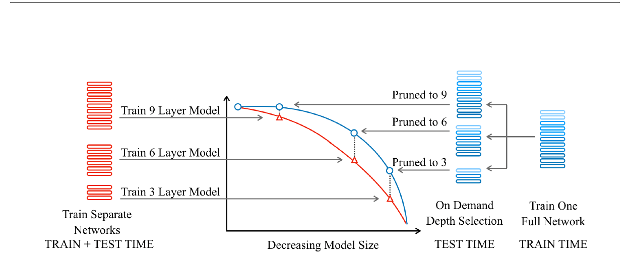
Source: Fan, Grave, and Joulin, Reducing Transformer Depth on Demand with Structured Dropout, Figure 1. Cropped from the official paper. The figure expresses the training objective’s purpose; a deployment still exports and validates one fixed selected subnetwork.

LayerDrop compares three inference-time selectors:

Selector	Evidence	Cost	Main risk
every other layer	balanced depth spacing	negligible	spacing is a heuristic, not task-specific evidence
search on validation	evaluate candidate layer subsets	combinatorial or search-dependent	expensive and can overfit the validation set
data-driven fixed top-$k$	learn per-layer drop-rate scores under an average-rate constraint	extra training and scoring	learned rule still requires a fixed export decision

The paper found every-other selection difficult to beat in its experiments and found consecutive first-half or last-half deletion harmful. These observations fit an ordered-composition view: early blocks process raw embedding state, late blocks prepare the final prediction state, and a long missing interval creates a larger adjacency shift than balanced omissions. They do not prove that every-other deletion is optimal for current decoder-only LLMs.

The Loop 7 fixture makes the expectation-versus-export distinction executable. For $N=4$ and $p=0.25$, it enumerates all $2^4=16$ binary masks rather than sampling them. Their probability mass is exactly $1$, while

E[K]   = 4 * (1 - 0.25)       = 3
Var[K] = 4 * 0.25 * (1-0.25) = 0.75

The fixed export used elsewhere in the fixture is a separate six-to-four decision, keep_old = [0, 2, 3, 5]. Matching an expected active depth during training does not create that ordered keep set.

LayerDrop is therefore a training-time robustness prior. It can be paired with balanced selection, validation search, learned fixed scores, or another post-training criterion. “Trained with LayerDrop” and “selected these layers” must remain two separate lines in an audit manifest.

0x07D Four Post-Training Scores Approximate Four Different Effects

For a pretrained checkpoint not prepared with LayerDrop, depth selection often uses calibration data. The following scores are not interchangeable.

One-Block Perplexity Ablation

Let calibration tokens be $x_1,\ldots,x_M$, and let $\theta_{\setminus \ell}$ denote the model with block $\ell$ replaced by identity. Its average next-token negative log-likelihood is

$$\mathcal L_{\setminus \ell} = -\frac{1}{M-1} \sum_{t=2}^{M} \log p_{\theta_{\setminus \ell}}(x_t\mid x_{<t}).$$

The corresponding perplexity is

$$\operatorname{PPL}_{\setminus \ell} = \exp\!\left(\mathcal L_{\setminus \ell}\right).$$

Since the exponential is monotone, ranking by $\operatorname{PPL}_{\setminus \ell}$ or $\mathcal L_{\setminus \ell}$ is equivalent on the same calibration set. A low value means that this one-block ablation was less damaging. It is direct evidence for the model’s prediction objective, but it requires roughly $N$ ablated evaluations for $N$ blocks.

It is still local. In general,

$$\Delta\mathcal L_{\{i,j\}} \ne \Delta\mathcal L_{\{i\}} + \Delta\mathcal L_{\{j\}},$$

because after removing $i$, block $j$ receives a different representation. A one-shot ranking must be followed by joint-subset validation; iterative rescoring is an alternative with higher calibration cost.

Gate Taylor Evidence

The exact whole-block counterfactual can also be relaxed to $z_\ell\in[0,1]$. A first-order expansion around the full model gives

$$\mathcal L(z_\ell=0) - \mathcal L(z_\ell=1) \approx -\left. \frac{\partial\mathcal L}{\partial z_\ell} \right|_{z_\ell=1}.$$

An absolute first-order block score is therefore

$$I_{gate,\ell} = \left| \left. \frac{\partial\mathcal L}{\partial z_\ell} \right|_{z_\ell=1} \right|.$$

This directly differentiates the identity-versus-block decision. Shortened LLaMA instead aggregates parameter-level Taylor products inside each block:

$$I_{Taylor,\ell} \propto \operatorname{Reduce}_{W\in B_\ell} \left| W\odot\frac{\partial\mathcal L}{\partial W} \right|.$$

The exact reductions over elements and matrices matter. Sum of absolute terms, absolute of a signed sum, mean, maximum, and product do not produce the same ranking. The official Shortened LLaMA code accumulates parameter-times-gradient state, takes absolute values and configurable norms at output-neuron level, then exposes configurable weight-level and block-level reductions. “Taylor score” is therefore incomplete without those choices.

Parameter Magnitude

A data-free block magnitude score aggregates surviving block weights:

$$I_{mag,\ell} = \operatorname{Reduce}_{W\in B_\ell}|W|^q.$$

It is cheap, but it measures parameter coordinates rather than the complete function delta $\Delta_\ell(h)$. LayerNorm/RMSNorm, residual scaling, matrix shape, and parameterization can make equal norms produce different hidden-state effects. Shortened LLaMA’s Mag+ and Taylor+ variants preserve the first four and last two blocks by excluding them from candidate deletion, because the raw metrics could rank boundary blocks as removable even when ablation quality said otherwise. That “plus” rule is a source-specific structural prior, not part of Taylor mathematics.

Block Influence

ShortGPT defines Block Influence for hidden row $X_{\ell,t}$ as cosine distance between the block input and output:

$$BI_\ell = 1- \mathbb E_{X,t} \left[ \frac{ X_{\ell,t}^{T}X_{\ell+1,t} } { \|X_{\ell,t}\|_2\|X_{\ell+1,t}\|_2 } \right].$$

Lower $BI_\ell$ means the block changes representation direction less on the calibration rows. All layer-boundary hidden states can be collected in one forward pass, making BI much cheaper than $N$ one-block PPL evaluations.

The geometric limitation follows from decomposing the block delta into parallel and orthogonal parts. Let

$$X_{\ell+1}=X_\ell+\delta, \qquad \delta=aX_\ell+\delta_{\perp}, \qquad X_\ell^T\delta_{\perp}=0.$$

Then

$$\cos(X_\ell,X_{\ell+1}) = \frac{(1+a)\|X_\ell\|_2} {\sqrt{(1+a)^2\|X_\ell\|_2^2+\|\delta_{\perp}\|_2^2}}.$$

For a small orthogonal change,

$$BI_\ell \approx \frac{\|\delta_{\perp}\|_2^2} {2(1+a)^2\|X_\ell\|_2^2}.$$

This explains what BI favors: low angular deflection relative to the residual state. If $X_{\ell+1}=cX_\ell$ for any positive $c$, BI is zero even though the norm changed. Conversely, a small orthogonal rotation can produce a nonzero BI without immediately proving a large next-token loss. BI is a useful proxy, not an identity test or a loss theorem.

The deterministic fixture applies all four score definitions to the same six blocks, calibration rows, objective, and full-model state. Lower-is-more- removable rankings are:

Score contract	Fixture ranking, lowest first
one-block objective loss	1, 4, 0, 5, 2, 3
absolute complete-gate Taylor	2, 5, 0, 3, 4, 1
parameter L1 magnitude	0, 3, 2, 5, 1, 4
row-wise block influence	0, 4, 1, 5, 3, 2

These are synthetic values, not paper-ranking reproductions. Their semantic purpose is that one shared input does not collapse four estimands into one order. The same fixture removes blocks 1 and 4 together: its actual pair loss is 0.013617906608, while adding their two isolated loss changes predicts 0.010770016105. That exact mismatch is the subset-interaction warning above.

0x07E ShortGPT Turns Hidden-State Geometry Into A Deletion Order

The ShortGPT paper applies the following pipeline:

unlabelled calibration text (PG19 in the paper)
    -> run the full model with all hidden boundaries returned
    -> compute one BI aggregate for every adjacent boundary pair
    -> sort block indices by ascending BI
    -> delete the requested number of lowest-BI blocks
    -> evaluate the joint shortened model

The paper’s Figure 3 compares BI with the PPL obtained by separately removing each layer. It is evidence from two source checkpoints, not a guarantee that BI and PPL correlate for every model or domain.

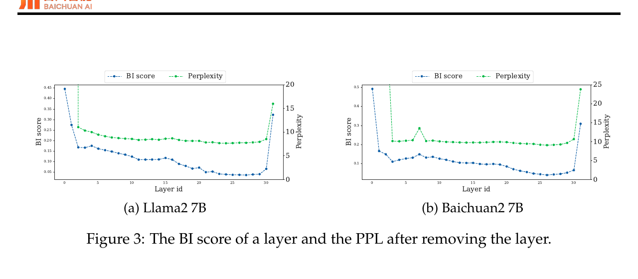
Source: Men et al., ShortGPT: Layers in Large Language Models are More Redundant Than You Expect, Figure 3. Cropped from the official paper. Both curves are source-reported calibration evidence.

The official code makes several implementation choices that should be visible in a reproduction:

# Conceptually equivalent, memory-linear BI accumulation.
def accumulate_bi(x_in, x_out, valid_tokens, total, count):
    # x_*: [batch, sequence, hidden]
    x = x_in.reshape(-1, x_in.shape[-1]).float()
    y = x_out.reshape(-1, x_out.shape[-1]).float()
    valid = valid_tokens.reshape(-1).bool()

    cosine = torch.nn.functional.cosine_similarity(x[valid], y[valid], dim=-1)
    total += (1.0 - cosine).sum(dtype=torch.float64)
    count += valid.sum()
    return total, count

bi = total / count.clamp_min(1)

The reference metrics.py flattens hidden rows, computes the full matrix input @ output.T, and takes only its diagonal. A row-wise dot product computes the same intended diagonal without materializing the quadratic token-by-token matrix. The reference accumulation uses a sum and replaces NaN similarity with 0.5; it also does not apply the tokenizer padding mask inside BI after the model forward. A robust reproduction should define zero-norm behavior, apply a valid-token mask, state sum-versus-mean reduction, and accumulate in adequate precision.

The official main path deletes entries from the layer container in reverse index order and then rewrites each surviving attention module’s layer_idx. Reverse deletion prevents earlier list indices from shifting before later deletions. The minimal mutation is:

drop = sorted(selected_original_indices, reverse=True)
for old_idx in drop:
    del model.model.layers[old_idx]

for new_idx, layer in enumerate(model.model.layers):
    layer.self_attn.layer_idx = new_idx

That is enough to change one in-memory Python graph, but not enough to define a portable release. A complete exporter must also set the configured layer count, preserve an original-to-new index map, migrate all layer-indexed state, save with the architecture metadata, and load the result in a fresh process.

At immutable ShortGPT commit 9a2ee8dfe9e28d0bee430e83c140b787c02ddd6c, the evidence path is split across four files: metrics.py:4-22 defines BI, shortgpt.py:26-47 ranks and deletes, run_shortgpt.py:9-38 fixes PG19 calibration and rewrites layer_idx, and shortgpt-gen/llama/shortgpt_llama.py:89-148 implements the non-equivalent phase-specific cache path described in 0x07G. Those line contracts are version-specific. They explain that repository revision; they are not generic Transformers APIs.

0x07F Shortened LLaMA Makes Runtime And Recovery Part Of The Choice

Shortened LLaMA focuses on a practical contrast. Width pruning keeps the number of block invocations but changes projection dimensions. Depth pruning keeps each surviving block’s native dense shapes but removes complete calls. On the small-batch GPU regimes studied in the paper, some narrowed shapes were less hardware-friendly while complete block deletion produced clearer latency gains. That is a measured result for the paper’s models, shapes, hardware, batch sizes, and software, not a theorem that depth always beats width.

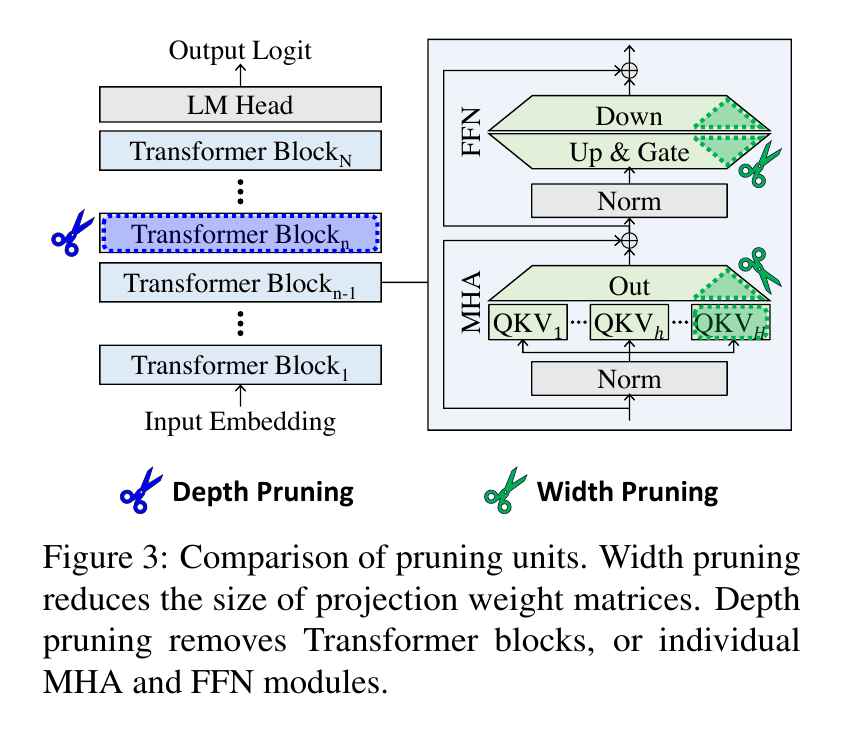
Source: Kim et al., Shortened LLaMA: Depth Pruning for Large Language Models with Comparison of Retraining Methods, Figure 3. Cropped from the official paper. The article keeps whole-block depth deletion separate from the head/channel surgery derived in Loop 5.

The paper studies four evidence families: magnitude, parameter Taylor, boundary-preserving Mag+/Taylor+, and one-block PPL. The official repository turns PPL scoring into an explicit $N$-model loop:

for original block index l:
    construct model with only block l removed
    run next-token loss on calibration samples
    store PPL_l and parameter count
sort original block indices by ascending PPL_l

Its exporter does not mutate the old ModuleList in place. It copies the configuration, decrements num_hidden_layers, constructs a new shorter model, and copies each surviving original block into a consecutive new index:

old 0 -> new 0
old 1 -> new 1
old 3 -> new 2       # old 2 removed
old 5 -> new 3       # old 4 removed
...

This is a stronger artifact boundary than deleting Python list entries alone: the saved configuration and state-dictionary namespaces agree on the new depth. It still needs modern cache, sharding, tied-state, adapter, and runtime tests when ported beyond the repository’s model/version assumptions.

The official Shortened LLaMA repository is pinned at 4031a9212aa0dbeec8f2ad504af9346c758b0147. Its code keeps the contracts separate: anal_block_sensitivity_ppl.py:73-167 constructs and evaluates one single-block deletion at a time; anal_block_sensitivity_taylor.py:94-189 and anal_block_sensitivity_magnitude.py:78-156 define different reductions; utils.py:114-171 rebuilds the shorter configuration and copies old -> new state; block_prune.py:63-107 applies the selected order and evaluates the artifact; and lora_retrain.py:108-234 trains, saves, and can merge adapter recovery. A ranking script, a converter, and a recovery script are therefore distinct executable stages, not one undifferentiated method.

Shortened LLaMA also makes recovery severity explicit:

Recovery path	Updated state	Cost character	Paper-scoped lesson
none	no surviving parameters	calibration/evaluation only	isolates immediate deletion damage
LoRA	low-rank adapter state on surviving projections	relatively light task/instruction recovery	competitive in some moderate-pruning settings studied
continued pretraining	all surviving base parameters	large corpus and optimizer state	substantially stronger for aggressive depth reduction in the paper
continued pretraining then LoRA	full-model recovery followed by task adaptation	combines both costs	separates language recovery from later instruction adaptation

The paper also compares removing complete blocks against removing attention or FFN modules separately and reports whole-block pruning as favorable in its studied regimes. That result is source-scoped. The mechanisms differ: module-level deletion can preserve more depth but creates mixed block types; whole-block deletion removes both branches and produces a regular shorter stack. Runtime regularity is part of the unit decision, not an afterthought.

0x07G “ShortGPT Runtime” Names Two Non-Equivalent Graphs In The Official Repository

The official ShortGPT repository contains a direct-deletion path and a separate shortgpt-gen experiment. They should not be described as one implementation.

Path One: Physical Depth Deletion

The main shortgpt path removes selected modules from model.layers. Once the configuration and serialization are repaired as described above, the runtime has $R$ block calls and $R$ cache layers. Both prefill and one-token decode use the shorter composition.

prefill:
    execute kept blocks only

decode:
    execute kept blocks only

KV schema:
    one cache slot per kept block

Path Two: Prefill-Only Full-Block Skip With Cache Projection

The repository’s custom LLaMA generation model keeps the original layer list. For a selected layer and a multi-token input, it skips the full block update but, when cache is enabled, still applies input normalization, K projection, V projection, reshape/transposition, RoPE metadata, and cache update. For a one-token input, its condition is false and the complete layer executes.

for layer_id, block in enumerate(model.layers):
    if q_len > 1 and layer_id in prefill_skip_set:
        if use_cache:
            x_norm = block.input_layernorm(hidden)
            k = block.self_attn.k_proj(x_norm)
            v = block.self_attn.v_proj(x_norm)
            cache.update(k, v, layer_id, rope_metadata)
        # hidden remains unchanged
    else:
        hidden = block(hidden, cache=cache, ...)

Its contract is therefore:

prefill:
    skip attention output + MLP for selected layers
    retain K/V projection and cache-write work for those layers

decode:
    execute all original layers

KV schema:
    retain original per-layer slots

This can be a valid experimental latency tradeoff, but it is not a physically shorter model and it does not have the depth-pruned KV equation from 0x07B. It also means the prefill and decode functions differ: decode revisits full blocks whose prefill cache was built from a hidden state that bypassed those blocks. Any article or benchmark must name which path was measured.

This distinction generalizes. A deployment can implement:

static physical deletion
fixed identity gates in a full graph
prefill-only skip with cache repair
decode-only skip
input-dependent routing

Only the first is the shorter static artifact owned by this section. Fixed gates are an oracle or transitional implementation. Phase-specific skipping is a runtime policy. Input-dependent routing belongs to M6.8.

0x07H Minitron Searches Architecture Tuples, Then Tests Them After Recovery

Minitron expands the decision from “which layers?” to “which architecture near a target parameter count?” A candidate can contain a depth $L$, embedding width $D$, MLP width $D_{ff}$, attention-head count $H_q$, and query-group count $H_{kv}$:

$$a=(L,D,D_{ff},H_q,H_{kv}).$$

Let $P(a)$ be the exact parameter count after applying all coupled tensor transformations. A simple feasibility band around target $P^*$ is

$$\mathcal A_{feasible} = \left\{ a:\left|P(a)-P^*\right|\le\epsilon P^* \right\}.$$

Enumerating only feasible tuples is important because one deleted block and one reduced MLP multiple do not remove equal parameter counts. It also prevents a quality comparison from quietly comparing different budgets.

For depth, the paper reuses one-block PPL and ShortGPT-style BI. For width, it uses forward-activation statistics over heads, neurons, and embedding channels. It then trims the selected architecture, performs lightweight retraining on every feasible candidate, reranks candidates, and spends the full retraining budget only on the selected architecture.

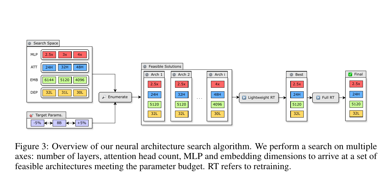
Source: Muralidharan et al., Compact Language Models via Pruning and Knowledge Distillation, Figure 3. Cropped from the official paper. RT in the figure means retraining.

The lightweight stage is not cosmetic. Minitron reports that candidate order can change during the first few hundred recovery steps in its studied search, including a width-versus-combined-depth/width ranking flip around 200 steps. The exact step and token counts are source-reported. The transferable lesson is that zero-shot post-prune loss may rank initialization damage, while the release objective cares about recoverable quality under a declared training budget.

Formally, a zero-shot selector chooses

$$a_0^*=\arg\min_{a\in\mathcal A_{feasible}}\mathcal L(a;\theta_a^0),$$

where $\theta_a^0$ is the immediately trimmed initialization. A recovery-aware selector instead approximates

$$a_s^* = \arg\min_{a\in\mathcal A_{feasible}} \mathcal L\!\left(a;\operatorname{Recover}_s(\theta_a^0)\right),$$

for a fixed short recovery budget $s$. These objectives need not have the same minimizer.

Minitron also compares one-shot and iterative importance estimation. Its reported recommendation favors single-shot importance for the model scales and budgets studied, and its paper recommends width over depth for the examined models up to 15B. Those are empirical design choices, not contradictions of Shortened LLaMA. The papers optimize different model families, workloads, hardware regimes, recovery budgets, and search axes. The correct conclusion is to include target runtime and recovery in the candidate objective.

The current NVIDIA NeMo pruning guide, last updated April 13, 2026, exposes three separate deployment operations:

target_num_layers
    -> BI-calibrated depth pruning

drop_layers
    -> caller-specified one-based layer indices

target hidden / FFN / head / query-group dimensions
    -> width pruning, optionally combined with depth

It also documents current API limits such as tp_size=1 for calibrated pruning and recommends distillation after pruning. These are versioned NeMo tool contracts, not properties of Minitron mathematics. The NVlabs Minitron repository primarily publishes papers, model links, and deployment entry points; the current executable pruning path is in NVIDIA’s NeMo/Model Optimizer stack. Paper method, released checkpoint, and current tooling must be cited as three different sources.

For auditability, the current guide was retrieved on August 12, 2026 as a 57,283-byte HTML snapshot with SHA-256 6af5228ff904b83a8c98df92f25a3346230442bbba81e1a435eb7d521275aa1e. That moving documentation record supports the current command/API boundary; it does not replace the immutable Minitron v2 paper. Likewise, the pinned NVlabs Minitron commit fed740c91886155e1f272159ef662536bb673593 contains a project README and released-model/deployment links, not the full paper pipeline implementation. The article therefore does not pretend that cloning that repository reproduces architecture search or distillation.

0x07I The Paper Variants Differ Across Five Contracts

Path	Preparation or evidence	Selection object	Immediate artifact	Recovery contract	Runtime claim boundary
LayerDrop	random structured layer masks during training	every-other, validation search, or learned fixed top-$k$	fixed shallower subnetwork selected from trained full model	main pruning comparisons often use none; appendices study fine-tuning	older Transformer tasks and implementations in the paper
ShortGPT main path	calibration hidden states and BI	lowest-BI individual blocks	layer entries deleted from in-memory stack	no mandatory recovery in core method	portable release needs config/cache/export work beyond minimal code
ShortGPT generation path	same chosen indices	fixed prefill skip set	full layer stack with phase-specific branch	not a depth-pruned checkpoint	selected prefill blocks still project/cache K/V; decode executes all layers
Shortened LLaMA	magnitude, Taylor, boundary-preserving variants, or one-block PPL	one-shot complete blocks, with optional protected endpoints	newly constructed shorter model and copied survivor weights	none, LoRA, CPT, or CPT then LoRA	depth-vs-width timings are hardware, shape, batch, and software scoped
Minitron	BI/PPL for depth plus activation evidence for width	feasible architecture tuple under parameter budget	trimmed depth/width candidate	lightweight candidate recovery then full KD/retraining	paper family creation plus current NeMo versioned tooling

Several alternatives remain valid:

• balanced fixed deletion avoids calibration scoring but encodes a spacing prior;
• contiguous-block deletion reduces the search description but creates a large representational jump and was harmful in LayerDrop’s experiments;
• one-shot ranking is cheap but ignores subset interaction;
• iterative rescoring observes changed adjacencies but costs repeated calibration and can depend on the deletion path;
• joint subset search can optimize the actual set but is combinatorial;
• learned gates can optimize depth under a resource loss and belong to Loop 8 when their schedules and exact-budget projection are derived;
• module-level depth pruning can remove attention or MLP independently but produces heterogeneous blocks and a different cache/runtime contract;
• layer merging or collapse transfers deleted transformations into survivors and is not pure deletion.

The selection report must state which alternative was used and why its cost is included or excluded.

0x07J Export Reconstructs A New Layer Namespace

A portable export needs enough immutable state to replay the conversion rather than infer it from tensor-key gaps:

@dataclass(frozen=True)
class DepthPruningManifest:
    source_checkpoint_sha256: str
    source_depth: int
    target_depth: int
    keep_old: tuple[int, ...]
    old_to_new: tuple[tuple[int, int], ...]
    selection_method: str
    calibration_sha256: str
    score_reduction: str
    artifact_class: str
    recovery_recipe: str
    converter_version: str

    def validate(self):
        assert self.keep_old == tuple(sorted(set(self.keep_old)))
        assert self.target_depth == len(self.keep_old)
        assert tuple(old for old, _ in self.old_to_new) == self.keep_old
        assert tuple(new for _, new in self.old_to_new) == tuple(range(self.target_depth))
        assert self.artifact_class in {
            "physical_shorter_graph",
            "fixed_identity_gate_graph",
            "phase_specific_skip_graph",
        }

artifact_class is required because the same keep indices can describe different parameter residency, cache schemas, prefill work, and decode work.

For original blocks 0..N-1, define sorted keep indices and an explicit map:

keep_old = sorted(set(keep_old))
assert keep_old and keep_old[0] >= 0 and keep_old[-1] < old_depth

old_to_new = {old: new for new, old in enumerate(keep_old)}
new_to_old = list(keep_old)

A safer generic export constructs a new model from the new configuration and copies state by semantic ownership rather than relying on list mutation:

new_cfg = deepcopy(old_model.config)
new_cfg.num_hidden_layers = len(keep_old)
new_model = ModelClass(new_cfg)

copy_non_layer_state(new_model, old_model)
for new_idx, old_idx in enumerate(keep_old):
    copy_block_state(
        dst=new_model.layers[new_idx],
        src=old_model.layers[old_idx],
    )
    set_runtime_layer_id(new_model.layers[new_idx], new_idx)

manifest = {
    "source_depth": old_depth,
    "target_depth": len(keep_old),
    "new_to_old_layer": keep_old,
    "selection_method": selection_method,
    "calibration_digest": calibration_digest,
    "recovery_recipe": recovery_recipe,
}
save_model_config_state_and_manifest(new_model, manifest)

The migration closure includes:

State	Required action
model configuration	update depth and any architecture-specific layer metadata
state-dictionary keys	rename each surviving layers.old.* namespace to layers.new.*
cache layer IDs	allocate only kept slots and use new consecutive runtime IDs
adapters	merge before deletion, delete removed-layer adapters, or rename survivor keys
quantization state	discard removed-layer scales and rename surviving per-layer metadata
optimizer/master weights	rebuild or map survivor parameter objects; never load deleted state by position
tied/shared state	preserve aliases rather than duplicating tensors during copy
tensor parallelism	surviving block tensor shapes can keep the same TP scheme, but shards and keys must be regenerated if serialization is layer-indexed
pipeline parallelism	repartition $R$ blocks; avoid empty or severely imbalanced stages
compiled/CUDA graphs	invalidate and recapture for the shorter call graph and cache schema
telemetry	preserve original-layer provenance while reporting new runtime layer IDs

The Loop 7 fixture compacts keep_old = [0, 2, 3, 5] as old_to_new = {0:0, 2:1, 3:2, 5:3}. It applies the same map to model-state prefixes, adapter prefixes, quantization prefixes, and cache slots. The resulting artifact ledger keeps three cases separate:

Synthetic artifact	Stored layers	Prefill full-block calls	Prefill K/V writes	Decode full-block calls	Cache slots	Parameters
physical shorter graph	4	4	4	4	4	190
fixed identity gates in full graph	6	4	4	4	6	235
ShortGPT-style prefill skip	6	4	6	6	6	235

The parameter fixture uses P_fixed = 100 and per-block counts [20, 21, 22, 23, 24, 25]; its values are pedagogical rather than model measurements. The call/cache differences, however, encode the graph contracts from 0x07B and 0x07G exactly.

Token positions do not require a layer-offset correction. RoPE, ALiBi, and causal-mask positions index sequence tokens, not graph depth. What changes is the semantic “depth” at which a surviving block now operates. Learned layer-specific biases, per-depth scalars, adapters, cache IDs, and diagnostics must follow the original-to-new map.

Pipeline balance deserves an explicit equation. If stage $s$ receives kept layer set $\mathcal K_s$, its work is approximately

$$C_s=\sum_{\ell\in\mathcal K_s}C_\ell.$$

End-to-end pipeline time is constrained by the slowest stage and bubbles:

$$C_{PP}\gtrsim\max_s C_s+C_{bubble}.$$

Deleting layers without repartitioning can leave one stage nearly empty while another remains the bottleneck. A lower total block count does not guarantee a proportional distributed speedup.

0x07K Recovery Must Match Deletion Severity And Release Objective

The immediate shortened model has two kinds of shift:

capacity shift
    -> fewer nonlinear transformations and fewer parameters

adjacency shift
    -> surviving block k receives a representation from an earlier original
       block than it saw during full-model training

LayerDrop attacks adjacency shift during original training. Post-training methods instead rely on low-sensitivity selection and optional recovery. Recovery choices change the claimed method cost:

no update
    -> cleanest test of score + deletion, weakest correction ability

LoRA / adapters
    -> low trainable state; base survivors remain frozen

continued pretraining
    -> all survivor weights can absorb changed adjacency and lost capacity

knowledge distillation
    -> teacher targets can constrain logits and selected intermediate states

architecture-search warmup
    -> short equal-budget recovery estimates which candidate is recoverable

M6.10 owns KL, hidden-state, relation, and on-policy distillation derivations. Depth pruning adds one mapping problem before using them. If student block $j$ originated from teacher block $k_j$, an original-index mapping is

$$\pi(j)=k_j.$$

A hidden loss can compare survivor-aligned states,

$$\mathcal L_{hid} = \sum_{j\in\mathcal H} \left\| P_j h_j^{student} - h_{\pi(j)}^{teacher} \right\|_2^2,$$

or use uniformly spaced/learned teacher targets instead. These mappings answer different questions. Original-index alignment preserves lineage; uniform mapping spreads supervision across teacher depth; learned mapping adds state and optimization. The map must be declared rather than inferred from the new consecutive student index.

Recovery data must also be separated from calibration data. Ten or a thousand short calibration examples may be sufficient to estimate a ranking but are not automatically sufficient to restore language modeling, long-context, multilingual, code, or safety behavior. Evaluation must include domains not used to select the blocks.

0x07L Evaluation Must Compare Architecture, Selection, And Training Budget

A fair depth-pruning experiment needs more than original-versus-pruned quality:

Comparison	Question isolated
original full model	total quality and runtime change
same target depth trained from scratch	value of inheriting survivor weights
balanced/every-other deletion	value of the learned or calibrated selector
random subsets with several seeds	robustness of the selected order
width-pruned model at matched parameters	depth-versus-width artifact and runtime
same target architecture with equal recovery tokens/FLOPs	value of initialization and objective rather than training budget
no-recovery versus LoRA/CPT/KD	where quality restoration comes from

The runtime report should include:

parameter bytes and serialized bytes
resident weight and runtime-buffer memory
KV bytes per token and actual number of cache layers
prefill latency at declared prompt lengths and batch sizes
decode inter-token latency at declared cache lengths and batch sizes
throughput under scheduler and concurrency targets
pipeline/tensor-parallel placement and communication
compile/capture warmup and graph reuse
quality before recovery and after each recovery phase
calibration, search, recovery, and conversion cost

Depth pruning can preserve familiar GEMM dimensions, which may avoid some width-pruning alignment failures. It also reduces sequential block calls and layer-stack cache. But fixed embeddings/head work, host scheduling, sampling, communication, pipeline bubbles, and memory allocation remain. The measured speedup is workload-specific.

0x07M Layer-Pruning Failure Lab

Failure	Silent cause	Observable consequence	Repair
delete a residual block and claim exact equivalence to the original model	shape-valid identity confused with learned block function	unexplained quality loss called a converter bug	compare physical export first to the same gate-zeroed dense model
gate attention or MLP and call it whole-layer deletion	removal unit changed	score and runtime do not match declared method	gate complete $B_\ell(h)-h$ or name the submodule unit
rank with one-block PPL and assume scores add	changed adjacencies create interaction	jointly deleted subset degrades unexpectedly	validate the subset; optionally rescore after each removal
treat BI as output equality	cosine ignores positive rescaling and downstream loss	low-BI layer can still affect logits	combine with ablation/held-out evaluation and state the geometric proxy
compute BI through a full token-token Gram matrix	only diagonal row pairs are needed	quadratic temporary memory	use row-wise cosine and a valid-token mask
include padding rows or silently replace zero-norm rows	calibration reduction undefined	data/batch formatting changes layer order	mask invalid rows and declare numerical fallback
train with LayerDrop and assume it selected the export subset	robustness prior confused with inference selector	arbitrary fixed graph	state every-other/search/data-driven selection separately
remove a contiguous first or last region without validation	endpoints and long adjacency jump ignored	severe task or LM degradation	protect boundaries only as an explicit prior and validate alternatives
delete ModuleList entries but leave old config depth	runtime graph and serialized architecture disagree	fresh load expects missing tensors or reconstructs old depth	rebuild from updated config and test fresh-process load
forget layer_idx and cache renumbering	cache keys use original positions	wrong cache writes, empty slots, or decode failure	serialize old/new maps and allocate consecutive runtime slots
call prefill-only skipping a shorter model	original layers still execute at decode and may still write K/V	theoretical depth/KV saving does not appear	name phase-specific runtime and measure each phase separately
reuse optimizer/LoRA/quant keys by new ordinal position	survivor identity changed after compaction	state from old layer 3 lands on old layer 4	migrate by original identity, then rename explicitly
keep old pipeline partition	total depth changed but stage assignment did not	empty stages or a new straggler	repartition by measured per-layer cost and recapture graphs
compare architecture candidates only immediately after trimming	ranking measures initial damage	selected candidate loses after equal recovery	use fixed-budget lightweight recovery before final selection
claim depth beats width from one paper	hardware, batch, shape, and recovery regime omitted	non-portable deployment choice	benchmark matched artifacts in the actual runtime
count $R/N$ as whole-model compression	embeddings and head are fixed	parameter and byte saving overstated	use $P_{fixed}+\sum_{\ell\in\mathcal K}P_\ell$
claim layer deletion changes RoPE positions	graph depth confused with token position	unnecessary or wrong positional remapping	keep token positions; migrate only layer-indexed state

0x07N Loop Boundary

Loop 7 has now followed depth pruning end to end:

define complete-block identity counterfactual
    -> B_l^z(h) = h + z_l(B_l(h)-h)

prepare or rank
    -> LayerDrop missing-layer training
    -> BI hidden-direction proxy
    -> one-block PPL ablation
    -> Taylor/magnitude proxies
    -> recovery-aware architecture search

select and validate
    -> preserve original order
    -> distinguish one-shot, iterative, balanced, and joint search
    -> test the complete selected subset

export
    -> construct shorter config and ModuleList
    -> copy survivors through an original-to-new map
    -> migrate cache, adapters, quantization, optimizer, TP/PP, and graphs

prove
    -> gate-zero parity
    -> fresh-process load and cached decode
    -> held-out quality before and after declared recovery
    -> prefill/decode/cache/distributed runtime measurement

Loop 8 returns to training-time selection, but at a different granularity. It owns relaxed and hard-concrete gates, movement scores, pruning schedules, resource penalties, exact-budget projection, mask freezing, and regrowth. The depth gate derived here supplies one possible structural unit; Loop 8 explains how such gates are optimized rather than assuming a post-training rank.

0x08 Training-Time Pruning Learns A Decision Process, Not Just A Score

The previous loops mostly began from a trained checkpoint, estimated which units could disappear, and then converted that decision into an artifact. Training-time pruning changes the order. A score or gate participates in the optimization itself, the active subnetwork changes while ordinary weights are still learning, and the eventual export decision may differ from the relaxed state used during training.

The owner question is therefore larger than “which score is highest?”:

How can binary keep/remove decisions receive useful gradients, how should the allowed budget change over training, how does a target parameter count differ from a target architecture, and which state must be frozen or converted before the result is a runnable pruned model?

This loop follows two methods deeply because they answer different versions of that question:

Movement Pruning
    -> learn one score per removable weight during task fine-tuning
    -> use a straight-through binary mask
    -> control a keep fraction with a warmup / cubic prune / cooldown schedule
    -> produce unstructured zeros unless a later representation changes

Sheared LLaMA
    -> learn hard-concrete gates over layers, residual coordinates,
       attention heads, and MLP intermediate coordinates
    -> constrain each gate family toward a pre-specified target shape
    -> deterministically project and physically slice a compact dense model
    -> continue pretraining with dynamically adjusted domain proportions

They should not be blended into a generic learned-mask method. Movement Pruning was evaluated primarily in a BERT transfer regime and its original unit is an individual weight. Sheared LLaMA starts from a decoder-only source LLM and searches a smaller structured target architecture. Their masks, schedules, optimizers, recovery budgets, and runtime artifacts differ.

The implementation statements below are revision-scoped. The Movement path is read against huggingface/block_movement_pruning commit c16cecafb9db2636250487064e00896a77772a3a: the schedule and cached global threshold live in masked_run_glue.py, STE decisions in binarizer.py, dense masked execution in masked_nn.py, and zero-valued export in bertarize.py. The Sheared path is read against princeton-nlp/LLM-Shearing commit b87218b566c73f6b246aaad3e4c42883f65a48a6: l0_module.py owns gate and constraint state, train.py owns minimizing versus maximizing optimizer groups, composer_llama.py and post_pruning_processing.py own structural conversion, and the callbacks and launch scripts own data-mixture and stage state. These are source traces, not claims that either repository was executed here.

0x08A Four States Must Remain Separate

A training-time pruning implementation usually contains at least four kinds of state:

State	Example	What it proves	What it does not prove
latent decision state	movement score $S$ or hard-concrete logit $\log\alpha$	the optimizer can rank or relax removal decisions	an exact deployed budget
forward state	binary $M$, sampled $z$, or soft deterministic gate	which paths contribute to this forward pass	a smaller checkpoint or faster operator
optimizer state	moments for $W$, $S$, $\log\alpha$, and constraint multipliers	how the decision can continue moving	that a frozen mask cannot regrow through stale state
exported state	zeroed dense weights, packed sparsity, sliced tensors, shorter layer list	what the loader reconstructs	that the target runtime selects a faster kernel

These states can disagree without a software error. A hard-concrete sample can be fractional during training, a deterministic evaluator can force an exact number of zeros, and the checkpoint can still contain the full source weights plus every gate. Conversely, a movement mask can have an exact top-$k$ count while its dense F.linear call executes the original matrix shape.

A minimal manifest therefore records all four:

decision_state:
  family: movement_score | hard_concrete_loga
  granularity: scalar | block | head | mlp_channel | hidden | layer
forward_mask:
  mode: sampled | local_topk | global_threshold | deterministic_exact_count
  schedule_step: 1840
  achieved_count_by_group: {...}
optimizer_state:
  weight_group: present
  gate_group: present
  multiplier_group: present | absent
  frozen_at_step: null
export_state:
  form: dense_zero | packed_sparse | physically_sliced_dense
  source_to_target_indices: {...}
  target_config: {...}

The persisted contract should be typed rather than inferred from a collection of tensor names:

@dataclass(frozen=True)
class TrainingPruningManifest:
    method: str
    source_checkpoint_sha256: str
    decision_state_kind: str
    decision_granularity: tuple[str, ...]
    schedule_kind: str
    schedule_state: dict[str, float | int]
    optimizer_group_roles: tuple[str, ...]
    current_mask_sha256: str
    frozen_indices_sha256: str | None
    target_config_sha256: str | None
    data_mixture_sha256: str
    used_sample_ids_sha256: str
    export_form: str | None

schedule_state and data_mixture_sha256 are resumable state, not descriptive metadata. Two checkpoints with equal weights but different cached thresholds, multiplier signs, gate RNG state, domain proportions, or used-sample cursors do not continue the same pruning process.

0x08B Why Movement Scores Measure A Trajectory

Consider one masked linear output coordinate:

$$a_i = \sum_j W_{ij}M_{ij}x_j, \qquad M=\operatorname{TopKeep}_{\kappa}(S),$$

where $S$ is a trainable score matrix and $\kappa\in[0,1]$ is the fraction kept. The forward mask is discrete: the largest $\lfloor\kappa |S|\rfloor$ scores survive. Ordinary differentiation through that ordering operation gives zero almost everywhere, so hard Movement Pruning uses a straight-through estimator (STE): during the backward pass, the discrete mask is treated approximately as if its derivative with respect to the score were one.

Let

$$\delta_i=\frac{\partial\mathcal L}{\partial a_i}.$$

The STE score derivative is then

$$\frac{\partial\mathcal L}{\partial S_{ij}} \approx \delta_i W_{ij}x_j.$$

For comparison, the ordinary masked-weight derivative is

$$\frac{\partial\mathcal L}{\partial W_{ij}} = \delta_i M_{ij}x_j.$$

Define the gradient that the unmasked connection would have received as

$$g^{dense}_{ij}=\delta_i x_j.$$

The score update becomes

$$S_{ij}^{(t+1)} = S_{ij}^{(t)} - \eta_S g_{ij}^{dense,(t)}W_{ij}^{(t)}.$$

Unrolling $T$ score updates gives

$$S_{ij}^{(T)} = S_{ij}^{(0)} - \eta_S \sum_{t=0}^{T-1} g_{ij}^{dense,(t)}W_{ij}^{(t)}.$$

This is the important derivation. A movement score is not $|W_{ij}^{(T)}|$, and it is not simply $|W_{ij}^{(T)}-W_{ij}^{(0)}|$. It accumulates a signed, data-dependent, optimizer-dependent first-order signal along the fine-tuning trajectory.

Under gradient descent, the sign cases are:

Current weight	Dense gradient	Weight update direction	$g^{dense}W$	Score update	Interpretation
$W>0$	$g<0$	more positive	negative	increases	moves away from zero
$W<0$	$g>0$	more negative	negative	increases	moves away from zero
$W>0$	$g>0$	less positive	positive	decreases	moves toward zero
$W<0$	$g<0$	less negative	positive	decreases	moves toward zero

This interpretation assumes the simple SGD sign relation for exposition. Momentum, adaptive preconditioning, decoupled weight decay, clipping, mixed precision, and gradient accumulation change the realized weight trajectory. The score remains a training-process quantity; it cannot be reconstructed from the final checkpoint weights alone.

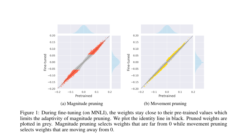
Source: Sanh, Wolf, and Rush, Movement Pruning: Adaptive Sparsity by Fine-Tuning, Figure 1. Cropped from the official paper. The scatter is source-reported for the studied BERT/MNLI setting; it is not a universal distribution of LLM weight motion.

The conceptual contrast is now precise:

magnitude score
    snapshot: |W_T|
    evidence: current parameter-space distance from zero

movement score
    trajectory: S_0 - eta_S * sum_t g_dense_t * W_t
    evidence: signed first-order pressure accumulated during adaptation

0x08C The Full Movement Schedule: Warmup, Cubic Pruning, Cooldown

The paper inherits gradual pruning from Zhu and Gupta. The notation is easy to misread because some pruning literature schedules sparsity, while the official Movement implementation passes the scheduled value to top-$k$ as the fraction retained. This article uses $\kappa(t)$ for keep fraction and $s(t)=1-\kappa(t)$ for sparsity.

Let:

t_0       first pruning step after the initial warmup
t_1       end of the pruning transition and start of cooldown
kappa_i   initial keep fraction
kappa_f   final keep fraction

The complete schedule is

$$\kappa(t) = \begin{cases} \kappa_i, &t\le t_0,\\[4pt] \kappa_f + (\kappa_i-\kappa_f) \left(1-\dfrac{t-t_0}{t_1-t_0}\right)^3, &t_0<t<t_1,\\[9pt] \kappa_f, &t\ge t_1. \end{cases}$$

The corresponding sparsity is

$$s(t)=1-\kappa(t).$$

Each interval has a distinct job:

initial warmup
    train W and S before forcing difficult competition

cubic pruning phase
    reduce the retained budget while scores and weights co-adapt

final cooldown
    hold the final mask budget while the surviving subnetwork adapts

For a toy schedule with $\kappa_i=1$, $\kappa_f=0.1$, $t_0=100$, and $t_1=900$:

Step	Normalized pruning progress	Keep fraction $\kappa(t)$	Sparsity $s(t)$
100	0.00	1.0000	0.0000
300	0.25	0.4797	0.5203
500	0.50	0.2125	0.7875
700	0.75	0.1141	0.8859
900	1.00	0.1000	0.9000

The cubic curve changes the budget rapidly early in the pruning interval and approaches the final budget gently. It is not interchangeable with a linear schedule, and the cooldown is not ordinary learning-rate warmup under a new name. The Movement paper reports that a final cooldown helps in its studied high-sparsity setting; that is source-scoped empirical evidence.

A renderer-safe implementation is:

def movement_keep_fraction(step, warmup_end, prune_end,
                           initial_keep=1.0, final_keep=0.1):
    if step <= warmup_end:
        return initial_keep
    if step >= prune_end:
        return final_keep

    p = (step - warmup_end) / (prune_end - warmup_end)
    return final_keep + (initial_keep - final_keep) * (1.0 - p) ** 3

The official repository expresses $t_0$ and the cooldown length as multiples of its optimizer warmup-step argument, then returns both the threshold and a regularization coefficient. That is historical implementation behavior, not a mathematical requirement of Movement Pruning. A reproduction must log the actual step boundaries rather than record only “cubic schedule.”

0x08D Local Top-K, Global Top-K, And Exact-Budget Timing

For score group $G$ with $n_G$ entries, local hard movement keeps

$$k_G(t)=\left\lfloor \kappa(t)n_G\right\rfloor$$

entries inside every group. If every matrix is a group, each matrix receives the same density even if their score distributions differ.

Global top-$k$ concatenates score groups:

$$S_{global}=\operatorname{concat}(S_1,S_2,\dots,S_G),$$ $$M_g = \mathbf 1 \left[ S_g\ge \operatorname{KthThreshold}(S_{global},k_{global}) \right].$$

Global selection allows nonuniform layer density. It also introduces a distributed systems question: which process owns the concatenated scores, how often is the threshold recomputed, how are ties resolved, and is the threshold broadcast before the next forward?

The official Movement training script recomputes a global numeric threshold only every configured global_topk_frequency_compute steps and reuses the cached threshold between updates. Therefore:

at threshold-recompute step
    target count can be projected from the current global score order

between recomputations
    scores continue to move under a fixed numeric threshold
    achieved count can drift away from the nominal top-k count

This distinction is absent under a freshly recomputed local top-$k$ mask. “Uses global top-k” does not by itself prove that every training step has the exact global budget.

def global_threshold(score_tensors, keep_fraction):
    flat = torch.cat([s.reshape(-1) for s in score_tensors])
    keep = int(keep_fraction * flat.numel())
    # Stable tie policy should be explicit in a production implementation.
    return torch.topk(flat, k=keep, largest=True).values[-1]

if step % threshold_refresh == 0:
    tau = global_threshold(all_mask_scores, keep_fraction)
mask = score >= tau
log_achieved_count(mask)  # required even when tau is cached

The Movement paper reports local and global selection as similar in most of its studied regimes, with a more visible global advantage at extreme sparsity. That result does not establish local or global selection as universally preferable for decoder LLMs.

0x08E Hard Movement, Soft Movement, And Hard Concrete Solve Different Budget Problems

The Movement paper compares three trainable decision mechanisms:

Method	Forward decision	Gradient path	Budget control	Export implication
hard Movement	$M=\operatorname{TopKeep}_{\kappa(t)}(S)$	STE through top-$k$	direct count when top-$k$ is recomputed	binary zero mask
soft Movement	$M_{ij}=\mathbf 1[S_{ij}>\tau]$	STE through threshold	indirect through $\lambda_{mvp}$ and fixed $\tau$	binary zero mask
$L_0$ / hard concrete	sampled stretched-concrete gate	reparameterized relaxed gradient	indirect expected $L_0$, unless followed by projection/constraints	stochastic training gate, deterministic test/export gate

Soft Movement adds

$$\mathcal R_{mvp}(S) = \lambda_{mvp} \sum_{ij}\sigma(S_{ij})$$

to the task objective. Increasing $\lambda_{mvp}$ encourages fewer scores to remain above the threshold, but it does not analytically guarantee a requested integer count. The penalty coefficient is a control parameter, not the final sparsity itself.

Hard concrete instead samples a relaxed variable, stretches it beyond $[0,1]$, and clips it. It supplies a pathwise gradient and a closed-form expected nonzero probability. It is not “Movement with a smoother top-k”: its decision distribution and budget semantics are different.

The official block_movement_pruning repository also supports score tensors at a block granularity and expands each block decision over several scalar weights. That is an implementation extension. The classic paper’s central Movement derivation and reported transfer experiments use unstructured weight masks; block support should not be retroactively described as the original paper’s only unit.

0x08F A Code-Level Movement Step

The official implementation uses separate optimizer groups for ordinary model parameters and mask_scores. Its masked linear path computes a mask, expands block masks if configured, multiplies the dense weight, and calls an ordinary dense linear operator.

def hard_movement_step(model, batch, step, optimizer, schedule):
    keep = schedule(step)

    for layer in model.masked_linears():
        layer.mask = straight_through_topk(layer.mask_scores, keep)

    loss = model(batch).loss       # F.linear(x, mask * weight, bias)
    loss.backward()
    optimizer.step()               # distinct LR groups for W and S
    optimizer.zero_grad(set_to_none=True)

At tensor level, one route is:

x                    [B, T, d_in]
W                    [d_out, d_in]
S                    [d_out, d_in] or block-grid shape
M = topk_STE(S)       same shape as S
expand(M)             [d_out, d_in] when block scores are used
W_masked = M * W      [d_out, d_in]
y = linear(x,W_masked)[B, T, d_out]

The backward state needs a more careful trace:

active weight
    task gradient reaches W
    score gradient also reaches S through STE

masked weight
    ordinary task-gradient path to W is multiplied by M=0
    score gradient can still reach S through STE
    S may cross the selection boundary and reactivate the connection

optimizer caveat
    stale momentum, master weights, or decoupled decay may still alter stored W
    even when its current task gradient is zero

Thus Movement supports score-based regrowth, not necessarily continuous task-gradient training of the masked weight value. When a connection returns, its stored $W_{ij}$ may be stale relative to continuously active neighbors. The checkpoint must preserve both score and optimizer state if training is to resume with the same dynamics.

optimizer_groups = [
    {"params": ordinary_weights, "lr": weight_lr, "weight_decay": wd},
    {"params": mask_scores, "lr": score_lr, "weight_decay": 0.0},
]

checkpoint = {
    "model": model.state_dict(),       # includes W and S while pruning
    "optimizer": optimizer.state_dict(),
    "step": step,
    "keep_schedule": schedule.state_dict(),
    "global_threshold": cached_tau,
}

The paper’s task fine-tuning setup also freezes embeddings and prunes the fully connected encoder weights in the studied BERT variants. Distillation is an optional additional signal in those experiments; Movement’s score derivation does not itself require a teacher.

0x08G Freeze, Regrow, And Export Are Separate Policies

During the pruning transition, allowing scores to move lets a previously masked connection re-enter. At some point a deployment pipeline usually freezes the topology. That decision must name which state stops changing:

Policy	$W$ updates	score/gate updates	mask changes	Use
dynamic movement	yes for active weights	yes	yes	joint selection and adaptation
mask-frozen recovery	yes for retained weights	no	no	stabilize final subnetwork
full freeze	no	no	no	conversion/evaluation oracle
regrowth-enabled sparse training	method-specific	yes	yes	recover from earlier choices

Freezing only the visible mask tensor is insufficient if the next forward recomputes it from still-trainable scores. Freezing scores is insufficient if the optimizer can still apply stale state. A robust transition removes gate parameters from the optimizer, clears incompatible moments, persists the chosen indices, and asserts that repeated forwards reproduce the same mask.

def freeze_movement_topology(model, keep_fraction):
    manifest = {}
    for name, layer in model.named_masked_linears():
        mask = exact_topk_mask(layer.mask_scores.detach(), keep_fraction)
        layer.register_buffer("frozen_mask", mask)
        layer.use_frozen_mask = True
        layer.mask_scores.requires_grad_(False)
        manifest[name] = torch.nonzero(mask, as_tuple=False).cpu()
    rebuild_optimizer_without_mask_scores(model)
    return manifest

The export then chooses a representation:

dense zero export
    save W_export = M * W at original shape
    easiest parity path; ordinary dense kernels usually do original work

general sparse export
    pack retained values and row/column metadata
    needs compatible sparse operators and shape/workload proof

N:M projection
    re-project within each hardware-defined local group
    changes the learned global/local mask unless the training unit already matched N:M

structured slicing
    impossible for arbitrary scalar Movement masks without a new grouping rule

The official Movement repository explicitly uses dense PyTorch linear calls for its masked model and reports no significant inference speedup from that path. Its zeroed checkpoint and sparse-storage examples should be read as artifact demonstrations, not proof that a standard dense GEMM skips zeros.

0x08H Sheared LLaMA Targets A Shape, Not Merely A Sparsity Ratio

Movement asks which scalar weights survive a budget. Sheared LLaMA starts from a source Transformer with

$$(L_S,d_S,H_S,m_S)$$

for layer count, residual width, attention-head count, and MLP intermediate width, then declares a target

$$(L_T,d_T,H_T,m_T).$$

That target is stronger than a total parameter count. Two models can contain the same number of parameters while one has an irregular per-layer shape and the other has regular dense GEMMs compatible with an existing runtime.

The paper learns four principal gate families:

Gate	Shape	Scope	Physical dependency closure
$z^{layer}$	$[L_S]$	global layer set	complete attention+MLP blocks and layer-indexed state
$z^{hidden}$	$[d_S]$	shared across the network	embeddings, norms, every residual producer/consumer, output head
$z^{head}_\ell$	$[H_S]$ per layer	local	Q/K/V head outputs and O input slices
$z^{int}_\ell$	$[m_S]$ per layer	local	gated/up rows and down columns

The paper’s conceptual layer gate controls complete blocks. The official code also contains attention-layer and MLP-layer mask helpers, while the released pruning script selects [head, intermediate, layer, hidden]. The exact enabled gate list is configuration state, not something a reader should infer from the paper figure alone.

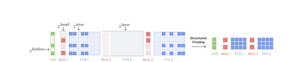
Source: Xia et al., Sheared LLaMA: Accelerating Language Model Pre-training via Structured Pruning, Figure 2. Cropped from the official paper. The diagram establishes the method’s target-shape and gate-family contract.

The paper’s source and target examples make the shape constraint concrete:

Model	Layers	Hidden	Intermediate	Heads	Head dimension
LLaMA2-7B source	32	4096	11008	32	128
Sheared-LLaMA-1.3B target	24	2048	5504	16	128
Sheared-LLaMA-2.7B target	32	2560	6912	20	128

These are source-reported configurations, not generally optimal Transformer ratios. The target inherits the source head dimension in this construction, so $H_T=d_T/d_h$ rather than choosing head count independently.

0x08I Hard Concrete Creates A Differentiable Gate With Atoms At Zero And One

For one gate logit $\log\alpha$, draw

$$u\sim\mathcal U(0,1).$$

The binary-concrete relaxation is

$$s = \sigma\!\left( \frac{\log u-\log(1-u)+\log\alpha}{\beta} \right).$$

Stretch it from $(0,1)$ to $(\gamma,\zeta)$ with $\gamma<0<1<\zeta$:

$$\bar s=s(\zeta-\gamma)+\gamma.$$

Then clip:

$$z=\min(1,\max(0,\bar s)).$$

The stretch matters. Values below zero collapse exactly to the atom at zero; values above one collapse to the atom at one; values in between remain differentiable relaxed gates. The reparameterized sample lets gradients reach $\log\alpha$ through $s$ before clipping.

The probability that the gate is nonzero is

$$\pi(\alpha) = P(z>0) = \sigma\!\left( \log\alpha - \beta\log\frac{-\gamma}{\zeta} \right).$$

Derivation: $z>0$ iff $\bar s>0$, which is equivalent to $s> -\gamma/(\zeta-\gamma)$. Applying the logistic inverse to that threshold and then the binary-concrete CDF yields the closed form above. This expected open probability lets the training objective estimate counts without sampling every possible discrete architecture.

The Sheared LLaMA paper reports

$$\beta=0.83, \qquad \zeta=1.1, \qquad \gamma=-0.1.$$

The historical official code uses bounds $[-0.1,1.1]$ but sets temperature to $2/3$. This is a paper/code difference that a reproduction manifest must resolve explicitly. The code also initializes gate logits around 5, clamps them to $[\log 10^{-2},\log 10^2]$, samples stochastic gates while training, and uses a deterministic path in evaluation.

def hard_concrete(log_alpha, beta, gamma=-0.1, zeta=1.1):
    u = torch.rand_like(log_alpha).clamp_(1e-6, 1 - 1e-6)
    logistic_noise = torch.log(u) - torch.log1p(-u)
    s = torch.sigmoid((logistic_noise + log_alpha) / beta)
    return (s * (zeta - gamma) + gamma).clamp_(0.0, 1.0)

def expected_open(log_alpha, beta, gamma=-0.1, zeta=1.1):
    return torch.sigmoid(log_alpha - beta * math.log(-gamma / zeta))

0x08J From Expected Gates To An Exact Target Architecture

An $L_0$ penalty controls the expected number of active gates indirectly. It does not say that every layer has exactly $H_T$ heads or $m_T$ intermediate coordinates. Sheared LLaMA instead constrains each gate family to match the declared target shape.

For heads in layer $\ell$, define the count residual

$$c_{head,\ell}(z) = \sum_{h=1}^{H_S}z^{head}_{\ell h}-H_T.$$

The paper writes a linear-plus-quadratic constrained term:

$$\widetilde{\mathcal L}_{head,\ell} = \lambda_{head,\ell}c_{head,\ell} + \phi_{head,\ell}c_{head,\ell}^2.$$

Analogous residuals enforce:

$$\sum_{\ell=1}^{L_S}z^{layer}_\ell=L_T,$$ $$\sum_{r=1}^{d_S}z^{hidden}_r=d_T,$$ $$\sum_{j=1}^{m_S}z^{int}_{\ell j}=m_T \quad\text{for each surviving layer }\ell.$$

The joint objective is a min-max problem:

$$\min_{\theta,\log\alpha} \max_{\lambda,\phi} \left[ \mathcal L_{LM}(\theta,z) + \sum_g \left( \lambda_g c_g(z)+\phi_g c_g(z)^2 \right) \right].$$

The model weights $\theta$ and gate logits minimize language-model loss plus constraint pressure. The multipliers ascend so persistent count error becomes more expensive. In the official optimizer builder, ordinary parameters use the model learning rate, gate parameters use lag_lr, and multiplier parameters use negative lag_lr; a minimizing optimizer thereby performs ascent on the multipliers.

groups = [
    {"params": theta,       "lr": model_lr},
    {"params": gate_logits, "lr": lag_lr},
    {"params": multipliers, "lr": -lag_lr},  # ascent
]

for batch in train_loader:
    z = {name: gate.sample() for name, gate in gates.items()}
    logits = model(batch.input_ids, gates=z)
    lm_loss = cross_entropy(logits, batch.labels)

    constraint_loss = 0.0
    for family in target_families:
        expected_count = expected_open_count(gates[family])
        target_count = scheduled_target_count(family, step)
        error = expected_count - target_count
        constraint_loss += lambda1[family] * error
        constraint_loss += lambda2[family] * error.square()

    (lm_loss + constraint_loss).backward()
    optimizer.step()
    clamp_gate_logits_()

This objective still operates on expected or relaxed state during training. Exact export requires a deterministic projection.

0x08K Sheared’s Schedule Is Not Movement’s Cubic Schedule

The official Sheared LLaMA $L_0$ module linearly warms the target sparsity for each gate family:

$$s_g^{target}(t) = s_g^{start} + \left(s_g^{final}-s_g^{start}\right) \min\left(1,\frac{t}{T_{lag}}\right).$$

The corresponding target count is

$$n_g^{target}(t) = n_g^{source}\left(1-s_g^{target}(t)\right).$$

This schedule changes the constraint target used by the Lagrangian. It does not itself select the bottom gates, and it is separate from the ordinary model learning-rate warmup.

Schedule	Controlled quantity	Curve	Decision rule
Movement	retained fraction $\kappa(t)$	constant / cubic / constant	top-$k$ score mask or threshold
Sheared	target sparsity/count residual	linear warmup then fixed	hard-concrete gates under constrained objective
ordinary optimizer	learning rate for weights/gates	implementation-specific	update magnitude, not architecture count

The released pruning script for the source-reported 7B-to-1.3B/2.7B runs uses 3,200 pruning batches, 10% ordinary LR warmup, and a 640-batch Lagrangian warmup. Those values describe that experiment and code release; they are not generic defaults for all target shapes.

0x08L Deterministic Projection And Physical Conversion

At evaluation, the official gate module computes a soft deterministic score from each logit. When target dimensions are configured, it then sets exactly the lowest

$$n_{zero}=n_{source}-n_{target}$$

scores to zero within each relevant row or global gate vector. Surviving scores are not necessarily one.

def deterministic_exact_target(log_alpha, target_count, beta):
    score = torch.sigmoid(0.8 * log_alpha / beta)  # official-code policy
    zero_count = score.numel() - target_count
    if zero_count:
        prune = torch.topk(score, k=zero_count, largest=False).indices
        score[prune] = 0.0
    return score

That means export has two operations, not one:

1. absorb any surviving fractional gate value into the adjacent weight;
2. physically remove zero-gated rows, columns, heads, channels, and layers.

For an intermediate gate $z^{int}$ in a gated MLP, for example:

$$W_{up}' = \operatorname{diag}(z_K)W_{up}[K,:],$$ $$W_{gate}'=W_{gate}[K,:],$$ $$W_{down}'=W_{down}[:,K],$$

where $K$ contains nonzero gate positions. The exact location at which a soft gate is absorbed depends on where it was applied in the forward graph. A converter cannot multiply every coupled matrix by the same vector without checking the algebra.

The historical official converter performs the dependency closure in code:

hidden gate
    multiply/slice token embeddings
    slice final norm and output-head input
    slice Q/K/V input axes and O output axis
    slice MLP input/output residual axes

head gate
    multiply selected head output where required
    slice Q/K/V output coordinates
    slice O input coordinates

intermediate gate
    absorb gate into the MLP path
    slice gate/up output rows
    slice down input columns

layer gate
    remove complete block state
    renumber surviving layer keys and runtime layer indices

The official post-pruning script loads the source-sized checkpoint with its gate module, requests deterministic masks, calls physical prune_params, removes the $L_0$ module, and saves the converted model. Before conversion, the pruning checkpoint can still contain the full source parameters plus mask state. Its file size is not the target model size.

A stronger conversion oracle is:

z_eval = gates.deterministic_exact_target()
y_masked = source_model(x, gates=z_eval)

target_model, index_map = physically_slice(source_model, z_eval)
y_sliced = target_model(x)

assert target_model.config == declared_target_config
assert_close(y_sliced, y_masked, atol=conversion_tolerance)

save(target_model, index_map, declared_target_config)
fresh = load_in_new_process(export_dir)
assert_close(fresh(x), y_sliced, atol=reload_tolerance)

The fresh target configuration is executable state. A state dictionary with smaller tensors cannot teach an ordinary source-model constructor which layers, heads, widths, or intermediate dimensions it should instantiate.

0x08M Dynamic Batch Loading Changes The Evidence Stream

After pruning, continued pretraining is not an incidental cleanup step in Sheared LLaMA. The paper treats it as the second major stage and changes the domain mixture according to validation deficits.

For domains $i=1,\dots,K$, let $w_i^{(t)}$ be the current sampling proportion, $\ell_i^{(t)}$ the current validation loss, and $\ell_i^{ref}$ a target reference loss. The paper’s Algorithm 1 defines

$$\Delta_i^{(t)} = \max\left(\ell_i^{(t)}-\ell_i^{ref},0\right),$$

then performs exponential reweighting:

$$\alpha_i^{(t)} = w_i^{(t-m)}\exp\left(\Delta_i^{(t)}\right),$$ $$w_i^{(t)} = \frac{\alpha_i^{(t)}}{\sum_j\alpha_j^{(t)}}.$$

A domain farther above its reference loss receives more probability. A domain already at or below the reference receives no positive deficit under the paper algorithm.

def paper_dynamic_mixture(current, val_loss, reference):
    deficit = torch.clamp(val_loss - reference, min=0.0)
    logits = torch.log(current) + deficit
    return torch.softmax(logits, dim=0)

The official callback differs in two visible ways:

def released_callback_mixture(current, val_loss, reference, floor=1e-4):
    diff = val_loss - reference          # no max(..., 0) clamp
    updated = torch.softmax(torch.log(current) + diff, dim=0)
    return (1.0 - floor) * updated + floor / updated.numel()

Therefore domains below reference can be downweighted relative to others, and a small uniform floor prevents complete disappearance. This is a meaningful paper/code distinction, not formatting noise. A reproduction should identify which update it runs.

The callback is applied during both pruning and continued pretraining. The CPT script starts from the final pruning-stage proportions rather than resetting to the original corpus mixture. Resume state also has to preserve used sample IDs; otherwise a resumed data stream can replay examples while appearing to resume the same optimizer step.

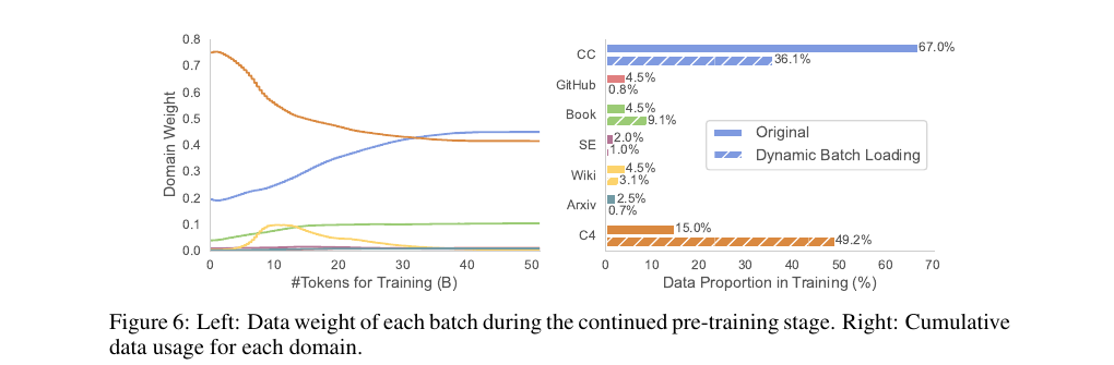
Source: Xia et al., Sheared LLaMA, Figure 6. Cropped from the official paper. The trajectories and percentages are source-reported for the paper’s RedPajama-domain experiment, not a recommended universal mixture.

Dynamic loading and mask learning are separate mechanisms:

gate optimizer
    changes which model substructures are likely to survive

dynamic loader
    changes which domains generate the next gradients

interaction
    changed data proportions change both ordinary weight gradients
    and the evidence received by pruning gates

The default reference losses in the paper are predicted per domain using a scaling-law fit:

$$\mathcal L(N,D) = E+\frac{A}{N^\alpha}+\frac{B}{D^\beta}.$$

The authors also study source-model validation losses as references. Both are source-scoped policy choices. The scaling-law fit is not ground truth for a hypothetical target architecture, especially when fitted from few model sizes.

0x08N The Full Sheared Training And Release State Machine

The complete method is easier to audit as a state machine:

# Stage 0: declare source and target architecture.
target = Shape(layers=L_T, hidden=d_T, heads=H_T, intermediate=m_T)
gates = make_gate_families(source_shape, target)

# Stage 1: targeted structured pruning.
for step, batch in pruning_stream:
    z = sample_hard_concrete(gates)
    lm_loss = source_model(batch, gates=z).loss
    lag_loss = target_shape_constraints(gates, target, step)
    backward_and_minmax_step(lm_loss + lag_loss)

    if step % eval_interval == 0:
        domain_losses = evaluate_each_domain(source_model, gates)
        pruning_stream.update_mixture(domain_losses, reference_losses)

# Stage 2: deterministic exact-count projection and conversion.
z_export = deterministic_target_masks(gates, target)
compact = absorb_soft_gates_and_slice(source_model, z_export, target)
remove_gate_modules(compact)
fresh_load_and_parity_check(compact)

# Stage 3: continued pretraining of the compact model.
for step, batch in continued_pretraining_stream:
    loss = compact(batch).loss
    loss.backward()
    optimizer.step()
    if step % eval_interval == 0:
        continued_pretraining_stream.update_mixture(
            evaluate_each_domain(compact), reference_losses
        )

# Stage 4: deployment proof.
measure_quality_before_and_after_cpt()
measure_prefill_decode_memory_and_throughput(compact)
ship_target_config_index_map_and_runtime_manifest()

The paper’s source-reported cost split is intentionally asymmetric:

Stage	Training budget	Weight LR	Gate/multiplier LR	Token batch	Steps	Reported throughput
targeted pruning	0.4B tokens	$10^{-4}$	1.0	131K	3,200	15K tokens/s
CPT, 1.3B target	50B tokens	$10^{-4}$	none	1M	51,200	145K tokens/s
CPT, 2.7B target	50B tokens	$10^{-4}$	none	1M	51,200	77K tokens/s

The paper reports pruning as roughly five times slower than ordinary LM training in its implementation because it carries source-model computation, stochastic gates, constraint state, and extra optimization. It allocates a small pruning budget because masks converge quickly, then spends most tokens recovering the compact model. These numbers are historical source-reported measurements on the paper’s hardware/software stack, not a capacity-planning estimate for a current cluster.

The accounting lesson is general:

$$C_{compression,total} = C_{search/prune} + C_{conversion} + C_{continued\ pretraining} + C_{evaluation}.$$

Reporting only the 0.4B pruning stage would hide the dominant 50B-token recovery budget. Reporting only final inference speed would hide the source model and gate-state training cost.

0x08O Movement Pruning And Sheared LLaMA By Contract

Contract	Movement Pruning	Sheared LLaMA
owner problem	task-adaptive sparse weight selection	source LLM to pre-specified compact dense architecture
original removal unit	scalar fully connected weight	layer, global residual coordinate, local head, local MLP coordinate
latent state	score $S_{ij}$	hard-concrete $\log\alpha$ per structure
gradient estimator	STE through top-$k$/threshold	reparameterized hard-concrete sample
budget	scheduled keep fraction or indirect threshold penalty	per-family target-shape constraints
schedule	warmup, cubic keep transition, cooldown	linear target-sparsity warmup plus ordinary LR schedule
exactness point	exact count when top-$k$ is freshly projected	deterministic lowest-score projection to target counts
regrowth	scores can cross selection boundary	gate probabilities can move before deterministic export
training model	masked source-shaped model	gated source-shaped model
initial artifact	dense weights multiplied by binary mask	full source checkpoint plus gates before conversion
release conversion	zero/pack according to sparse runtime	absorb residual gate values and slice coupled axes/layers
recovery	continued task fine-tuning; optional distillation in paper	dedicated continued pretraining stage
data adaptation	task dataset in paper	dynamic per-domain loading during pruning and CPT
default runtime shape	original dense shape unless packed operator changes it	smaller regular dense target shape after conversion
evidence boundary	BERT transfer tasks and studied sparsity regimes	LLaMA2-7B to paper target shapes and training stack

The common principle is only that removal decisions are learned jointly with model adaptation. Everything after that statement must remain method-specific.

The Loop 8 dependency-free fixture makes the distinctions executable. It does not train either paper model; it evaluates the exact equations on small fixed vectors and rejects one-field contract substitutions:

Contract	Deterministic fixture result	What the result prevents
Movement keep schedule	steps 0,2,4,6,8,10 retain 1,1,0.472222,0.277778,0.25,0.25	replacing warmup/cubic/cooldown with one linear ramp
masked backward	a masked weight has zero ordinary task gradient while its score receives a nonzero STE gradient	claiming score regrowth means masked weights train normally
local versus global top-k	two local groups retain [2,2]; global selection retains [4,0]	calling equal density and global competition equivalent
cached global threshold	exact count 4 at refresh drifts to 6; fresh top-k returns 4	claiming cached-threshold steps meet an exact integer budget
hard-concrete state	expected open count differs from deterministic export count; projection retains exactly 3 soft survivors	treating relaxed expectation as the exported architecture
multiplier optimizer	a minimizing optimizer with negative multiplier LR matches explicit ascent	silently descending every Sheared parameter group
conversion	five gated MLP coordinates slice to three with masked-versus-sliced maximum error below 1e-10	dropping surviving gate scales or slicing only one coupled tensor
dynamic loading	clamped paper deficits and released raw-difference-plus-floor updates produce different normalized mixtures	claiming paper and released callback equations are identical
lifecycle accounting	0.4B + 50B = 50.4B source-reported training tokens before conversion/evaluation costs	reporting only the mask-learning stage as compression cost

The fixture also round-trips domain proportions, used-domain IDs, and the evaluation cursor. That is a serialization invariant only. It does not prove the historical distributed loader, optimizer, model, or recovery run.

0x08P Training-Time Pruning Failure Lab

Failure	Silent cause	Observable consequence	Repair
call $S_T$ the final weight displacement	score trajectory confused with $W_T-W_0$	movement ranking cannot be reproduced	persist score state and derive $-\sum_t g_tW_t$ under the actual optimizer
schedule “90%” without saying keep or sparsity	top-$k$ threshold semantics inverted	retain 90% when intending to retain 10%	log both $\kappa(t)$ and $s(t)=1-\kappa(t)$
omit warmup/cooldown boundaries	cubic phase treated as complete schedule	reproduction prunes at different optimizer state	serialize exact $t_0,t_1$, total steps, and LR schedule
cache a global threshold and claim exact top-$k$ every step	scores move between threshold refreshes	achieved count drifts	log achieved count and recompute/project at required cadence
assume masked $W$ keeps learning normally	STE score gradient confused with weight gradient	regrown values are stale	distinguish task gradient to $W$ from score gradient to $S$
freeze the visible mask but retain score optimizer state	mask is recomputed on next forward	topology changes during recovery	freeze scores, remove optimizer group, persist exact indices
load a movement checkpoint and expect sparse speedup	dense linear(mask * W) remains	latency unchanged or worse	convert to supported packed format and prove kernel dispatch
call hard Movement, soft Movement, and $L_0$ equivalent	count projection and relaxed penalties conflated	final sparsity differs from request	state decision, gradient, and budget contracts separately
use total target parameters for Sheared LLaMA	architecture geometry omitted	irregular or unsupported runtime shapes	constrain layers, hidden width, heads, and MLP width explicitly
treat expected open count as exact export count	relaxed objective confused with discrete artifact	wrong target dimensions	run deterministic exact-count projection and validate config
discard nonbinary surviving gates before slicing	relaxed scale not absorbed	converter parity fails	multiply surviving scale into the correct adjacent weight first
slice only one tensor for a hidden/head/MLP gate	dependency closure ignored	shape mismatch or changed function	reuse Loops 5-7 coupled-axis closure and parity test
ship source-sized checkpoint plus gates as the target	training state confused with artifact	file and loader still instantiate source model	physically slice, remove gate module, and save target config
optimize all Sheared parameter groups with positive LR	max variables accidentally descend	constraints fail to enforce target	use explicit ascent or audited negative-LR multiplier group
cite paper $\beta=0.83$ while running code $2/3$ silently	paper/code drift hidden	gate distribution differs	pin and record the chosen implementation contract
implement paper dynamic loading but claim code parity	clamp and floor differences omitted	domain proportions diverge	test paper and released callback equations separately
reset data proportions at CPT	pruning-stage loader state discarded	recovery data trajectory changes	initialize CPT from final pruning proportions when reproducing paper
resume without sample-ID state	optimizer resumes but data stream repeats	token accounting and validation trajectory drift	checkpoint loader proportions and used-domain IDs
report only pruning tokens	CPT dominates but is hidden	compression cost understated	report prune, convert, CPT, evaluation, and deployment costs
transfer source-reported throughput to new hardware	implementation and cluster scope omitted	invalid capacity forecast	rerun end-to-end training and serving measurements

0x08Q Loop Boundary

Loop 8 has now followed training-time pruning from differentiable decision to release candidate:

Movement Pruning
    -> derive STE score gradient
    -> accumulate signed first-order trajectory
    -> warmup / cubic keep schedule / cooldown
    -> distinguish local, global, cached-threshold, and penalty budgets
    -> preserve score and optimizer state while regrowth is allowed
    -> freeze exact indices and choose a real sparse representation

Sheared LLaMA
    -> declare target layers, hidden width, heads, and MLP width
    -> sample hard-concrete structured gates
    -> minimize model/gate state and maximize constraint multipliers
    -> linearly warm target sparsity by gate family
    -> deterministically project exact target counts
    -> absorb soft survivors and slice every coupled tensor
    -> continue pretraining with checkpointed dynamic domain loading

release proof
    -> masked-versus-converted parity
    -> fresh-process target-config load
    -> quality before/after recovery
    -> measured artifact bytes, memory, prefill, decode, and throughput

Section 0x09 compares the complete LLM pruning pipelines by these contracts. It does not rank methods by one benchmark table. It owns the cross-paper matrix for LLM-Pruner, Sheared LLaMA, SliceGPT, Shortened LLaMA, ShortGPT, and Minitron: removal unit, evidence, target control, training/calibration data, conversion, recovery, artifact, and runtime claim.

0x09 A Pruning Paper Is A Pipeline Contract, Not A Method Label

The six LLM methods developed in Loops 5-8 are often placed in one benchmark table because every final model has fewer parameters. That shared endpoint is not enough to make the methods interchangeable. They begin from different source checkpoints, remove different graph objects, spend radically different amounts of data and training compute, export different runtime graphs, and measure speed under different workloads.

Owner question: what must be recorded, and what must be held constant, before two pruning papers can answer the same engineering question?

The answer is a pipeline contract. A score is one field in that contract, not the method itself. For this comparison, define

$$\mathcal P = (M_S,\mathcal U,\mathcal D_E,\mathcal S,\mathcal B, \mathcal F,\mathcal C,\mathcal R,\mathcal A,\mathcal V),$$

where:

Field	Question it fixes
$M_S$	Which exact source checkpoint and architecture are compressed?
$\mathcal U$	What graph object can be removed: block, head, MLP coordinate, residual direction, or a coupled group?
$\mathcal D_E$	Which examples, sequence lengths, masks, and reductions create pruning evidence?
$\mathcal S$	Is evidence magnitude, Taylor, ablation PPL, hidden geometry, activation energy, or a learned gate?
$\mathcal B$	Is the target a removed-parameter ratio, exact depth, exact per-axis shape, slicing schedule, or architecture search space?
$\mathcal F$	When and how is a discrete topology frozen?
$\mathcal C$	How are gates, indices, rotations, and source tensors converted into an executable graph?
$\mathcal R$	Is recovery absent, LoRA, full continued pretraining, distillation, or a staged combination?
$\mathcal A$	What is actually released: mutated source object, custom compressed module, or fresh standard target configuration?
$\mathcal V$	Which quality suite, hardware, runtime, dtype, batch, sequence shape, and serving phase support the claim?

Two papers are directly comparable only on fields that either match or are deliberately controlled. A matched final parameter count does not repair a mismatch in source model, recovery budget, or runtime workload.

The comparison record is therefore executable state, not an informal row in a spreadsheet:

@dataclass(frozen=True)
class PaperPipelineRecord:
    method_id: str
    paper_revision: str
    source_checkpoint: str
    source_geometry: dict[str, int]
    removable_unit: str
    evidence_manifest: dict[str, object]
    score_or_search: str
    target_contract: dict[str, object]
    freeze_rule: str
    conversion_contract: str
    immediate_artifact: str
    recovery_contract: dict[str, object]
    release_artifact: str
    evaluation_manifest: dict[str, object]
    workload_manifest: dict[str, object] | None

@dataclass(frozen=True)
class VectorBudget:
    evidence_tokens: int
    evidence_forwards: int
    evidence_backwards: int
    search_candidates: int
    recovery_tokens: int
    teacher_forwards: int
    trainable_parameters: int
    optimizer_state_bytes: int
    wall_time_seconds: float | None
    hardware_manifest: str | None

The nullable fields matter. An unavailable runtime measurement is None, not zero. A source-reported three-hour recovery run is not silently converted into a portable compute budget when sequence count, token count, kernel stack, and hardware utilization are missing. The record also separates the immediate post-conversion artifact from the recovered release, because those checkpoints answer different causal questions.

The comparison source surface is immutable. LLM-Pruner is consumed from the Loop 5 2305.11627v3 paper and commit-pinned code records; SliceGPT from the Loop 6 2401.15024v2 paper and 6b12cdee... code records; ShortGPT, Shortened LLaMA, and Minitron from the Loop 7 revision/code records; and Sheared LLaMA from the Loop 8 2310.06694v2 paper and b87218b... implementation records. Loop 9 compares those frozen contracts. It does not replace them with current repository heads, a new framework execution, or memory-based summaries of the papers.

0x09A Normalize Every Paper Into The Same State Machine

The common state machine is longer than score -> prune -> benchmark:

source checkpoint
    -> evidence acquisition
    -> candidate selection or topology search
    -> discrete topology freeze
    -> physical graph conversion
    -> optional recovery
    -> release packaging
    -> quality and runtime validation

Each arrow can change the model. Evidence acquisition may run only forwards, may require gradients, or may jointly train gates and weights. Topology search may choose coordinates inside a fixed target shape or compare several target architectures. Conversion may simply renumber surviving blocks, may slice a dependency closure, or may introduce executable shortcut matrices. Recovery may consume no data, 50K instruction examples, billions of language-modeling tokens, or teacher forwards over a large training run.

A reported number must attach to one state. For example, quality after pruning can mean the newly sliced graph before any update, the same graph after LoRA, or a compact model after 50B continued-pretraining tokens. Calling all three results pruned quality hides the causal difference.

0x09B The Six Complete Pipelines

The following table records the main paper path rather than every ablation. All data volumes, runtimes, and model names are source-reported and scoped to the corresponding paper.

Paper path	Evidence and target decision	Physical conversion	Recovery and released state	Evidence boundary
LLM-Pruner	discover coupled dependency groups; use 10 calibration samples of length 128 from BookCorpus for LLaMA/Vicuna or DailyDialog for ChatGLM; rank grouped structures with magnitude/Taylor variants under an approximate removed-parameter ratio	prune dependency-closed head/MLP or residual-channel groups; resulting widths can be heterogeneous; official paths include Python-object serialization and later architecture-specific support	optional LoRA on about 50K cleaned Alpaca examples for two epochs; paper reports about three hours on one GPU; merge adapters into the structurally smaller model	LLaMA-7B/13B, Vicuna-7B, ChatGLM-6B; paper Table 3 times a 64-token inference input on one A5000
Sheared LLaMA	jointly train hard-concrete layer, hidden, head, and MLP gates on RedPajama under exact target-family constraints; paper allocates 0.4B pruning tokens and chooses 1.3B/2.7B target shapes	deterministically retain exact counts, absorb surviving gate scales, slice every coupled tensor, remove gate modules, renumber layers, and load a fresh target configuration	full continued pretraining for 50B tokens with dynamic domain loading; released artifact is a regular smaller dense model at the declared target shape	LLaMA2-7B source; paper compares targeted and nonuniform pruning generation speed on one A100 80GB and reports downstream results for its data/training stack
SliceGPT	collect boundary activations, form uncentered Gram matrices, compute PCA bases, and apply a constant or configured residual-width slicing schedule; main experiments use WikiText-2 or Alpaca calibration, commonly 1,024 sequences of length 2,048 for LLaMA2	fuse normalization state, rotate each boundary, delete low-energy directions, and install dense square or rectangular residual shortcut transforms; custom compressed modules and a slicing config are executable architecture state	slicing can be evaluated without weight updates; optional LoRA recovery uses about 1K WikiText-2 or 5K Alpaca sequences; released state includes custom layer and shortcut parameters	OPT, LLaMA2, and Phi-2; paper reports batch-1, length-128 generation timing on A100/RTX6000 and max-throughput sweeps on H100, with explicit runtime caveats
ShortGPT	run an unlabeled PG19 calibration stream, collect block input/output hidden states, rank complete blocks by Block Influence, and remove the lowest scores to a requested depth ratio	direct path deletes entries from the layer stack; a distinct repository generation path performs phase-dependent skipping and is not the same shortened graph	no recovery is required by the core method; a separate paper experiment replaces removed blocks with lightweight gated MLPs and trains for 50B tokens, changing both architecture and budget	LLaMA2, Baichuan2, RWKV, and Mamba experiments; GPTQ throughput table and official phase-specific path must not be treated as one universal runtime artifact
Shortened LLaMA	use 10 BookCorpus calibration samples; rank whole blocks with magnitude, Taylor, protected-boundary variants, or one-block PPL; remove complete blocks once to meet a target parameter size	construct a fresh shorter configuration, copy surviving blocks, and remap old layer indices to consecutive target indices	compare no update, LoRA on 50K Alpaca examples, full CPT on SlimPajama, and CPT then LoRA; severe pruning conclusions depend strongly on the selected recovery path	LLaMA-7B and Vicuna-7B/13B; paper timing uses 12 input and 128 output tokens, batch 1, default Transformers, on H100 80GB and RTX3090 24GB
Minitron	use 1,024 calibration samples; rank width axes by activation evidence and depth by PPL or BI; enumerate feasible depth/width architecture tuples under a parameter budget; apply about 1.8B tokens of equal lightweight recovery to each candidate before final ranking	physically trim embedding, attention, MLP, and optional depth axes; an iterative family path prunes the already recovered 8B model to build the 4B model	full retraining is distillation-centered; the paper reports 94B training tokens for released Minitron models and recommends logits-only or added hidden/embedding targets according to depth change	Nemotron-4 15B source and Nemotron/Minitron family; paper reports quality and training evidence, but no direct end-to-end latency or throughput table for the released models

This matrix prevents six common substitutions:

ten calibration examples       != 50K recovery examples
50K instruction examples       != 50B pretraining tokens
one fixed target shape         != architecture search
deleting layer objects         != phase-specific layer skipping
custom dense shortcuts         != stock smaller Transformer
matched parameter count        != matched runtime graph

0x09C A Compression Ratio Does Not Identify The Compressed Graph

Let the source architecture geometry be

$$G_S=(L,d,H_q,H_{kv},d_h,m,\Gamma),$$

where $\Gamma$ contains per-layer overrides, endpoint policy, packed layouts, and custom shortcut state. The removed-parameter ratio is only

$$r_P=1-\frac{P(G_T)}{P(G_S)}.$$

It does not reveal which coordinate of $G$ changed. For a decoder with fixed embedding/head state $P_{fixed}$ and approximately uniform blocks,

$$P(G) \approx P_{fixed}(V,d) + L\left[ d^2 +2d(H_{kv}d_h) +d^2 +3dm \right].$$

The four attention terms correspond to Q, K, V, and O under a GQA-style layout; model-specific biases, norms, tied endpoints, and packings must be counted separately. The equation exposes why equal $r_P$ can create unlike systems:

• reducing $L$ removes complete sequential block calls and one persistent K/V cache layer per removed block while preserving surviving GEMM shapes;
• reducing $m$ shrinks three MLP matrix axes but leaves attention, layer count, and K/V layer count unchanged;
• reducing $H_q$ can shrink Q/O and query attention work without changing GQA K/V width;
• reducing shared residual width $d$ changes embeddings, projections, MLPs, endpoints, and possibly shortcut matrices with linear and quadratic terms;
• a hybrid target changes several terms and may preserve runtime alignment better than an arbitrary one-axis count.

Therefore a fair report includes the geometry delta, not only 20% pruned:

{
  "source": {"layers": 32, "hidden": 4096, "q_heads": 32, "kv_heads": 32, "mlp": 11008},
  "target": {"layers": 24, "hidden": 4096, "q_heads": 32, "kv_heads": 32, "mlp": 11008},
  "parameter_reduction": "measured from serialized tensors",
  "custom_shortcuts": false,
  "heterogeneous_layers": false
}

Replacing the target with hidden=3072, heterogeneous per-layer heads/MLPs, or per-boundary SliceGPT widths can reach a similar parameter count while changing kernel alignment, graph count, cache state, and loader requirements.

0x09D Coordinate Selection And Architecture Selection Are Different Searches

The methods solve three distinct search problems.

Fixed architecture, select surviving coordinates

Sheared LLaMA starts from a target tuple such as $(L_T,d_T,H_T,m_T)$ and learns which source structures fill it. SliceGPT receives a width schedule and chooses which rotated directions survive at each boundary. Shortened LLaMA receives a target depth or parameter size and chooses the surviving original blocks.

The target geometry is fixed before the final coordinate selection:

$$K^*(G_T) = \arg\min_{K\in\mathcal K(G_T)} \widehat{\Delta L}(M_S,K;\mathcal D_E).$$

Fixed unit family, choose a subset under an approximate budget

LLM-Pruner and ShortGPT rank dependency groups or blocks and remove low-scored units. Group sizes need not be equal, so a nominal parameter ratio can be an approximate stopping rule rather than an exact architecture equation.

Search architecture tuples, then select coordinates

Minitron enumerates feasible geometries first. Each candidate needs its own trimmed coordinates and equal lightweight recovery before comparison:

$$G_T^* = \arg\min_{G\in\mathcal G(P_{budget})} L_{val}\left( \operatorname{Recover}_{C_{light}} (\operatorname{Trim}(M_S,G)) \right).$$

Ranking unrecovered candidates instead would answer a different question: which topology suffers the smallest immediate damage. Minitron’s source- reported experiments show that candidate order can change during lightweight retraining, so post-pruning loss is not a reliable substitute for recovered architecture quality in that pipeline.

0x09E Recovery Is Part Of The Method Cost And Sometimes Part Of Selection

Use a full compression cost ledger:

$$C_{total} = C_{evidence} +C_{search} +C_{conversion} +C_{recovery} +C_{evaluation} +C_{release}.$$

For architecture search with $n$ candidates,

$$C_{search} = \sum_{a=1}^{n} \left(C_{evidence,a}+C_{light\ recover,a}+C_{validation,a}\right).$$

For distillation, training tokens alone also omits teacher work:

$$C_{KD} \approx C_{student\ train} +C_{teacher\ forward} +C_{state\ alignment} +C_{communication}.$$

The papers intentionally occupy different cost regimes:

Pipeline	Evidence/search update	Main recovery path in reported strong result	Accounting caveat
LLM-Pruner	gradients on 10 short public examples	LoRA, about 50K Alpaca examples, two epochs	three hours is a source-reported single-GPU experiment, not a hardware-independent budget
Sheared LLaMA	0.4B tokens of gated source-model pruning	50B tokens of full CPT with dynamic loading	pruning is reported around 5x slower than ordinary LM training; the 0.4B stage is not total cost
SliceGPT	activation collection and eigendecomposition; no base-weight update	optional LoRA on about 1K or 5K sequences	paper could not find beneficial RFT settings for OPT; slicing and RFT costs vary by model
ShortGPT	forward hidden-state collection	none in core path; separate 50B-token MLP-replacement experiment	replacement means the recovered artifact is no longer pure block deletion
Shortened LLaMA	forward or backward evidence on 10 examples	LoRA for moderate pruning; CPT or CPT then LoRA for severe pruning	paper reports CPT as far more expensive than LoRA and uses eight H100 GPUs for the studied runs
Minitron	1,024-example evidence plus about 1.8B tokens per searched candidate	large KD/retraining program; released tables report 94B training tokens	candidate warmups, family iterations, teacher forwards, and final training must not be collapsed into one token count

An equal-recovery comparison should snapshot every artifact immediately after conversion, then apply the same trainable-parameter policy, data, tokens, optimizer, and objective. A paper-faithful comparison is also valuable, but it answers which complete published pipeline performs best under each paper’s chosen cost, not which pruning decision is intrinsically best.

0x09F Runtime Evidence Is A Workload-Bound Contract

Define the deployment workload as

$$\mathcal W = (H,\mathcal R,\mathrm{dtype},\mathrm{quant},TP,PP,B,T_{in},T_{out},C,Q),$$

where $H$ is hardware, $\mathcal R$ is runtime/version, $B$ is batch or active sequence count, $T_{in}$ and $T_{out}$ are prompt and generation lengths, $C$ is concurrency/scheduler policy, and $Q$ is the quality checkpoint being timed. A speedup ratio is meaningful only relative to a baseline measured under the same $\mathcal W$.

Pipeline	Runtime evidence actually supplied	What it does not establish
LLM-Pruner	source-reported parameter, MAC, memory, and latency table for a 64-token input on one A5000	prefill/decode split, continuous batching, portable heterogeneous loading, or current-kernel speed
Sheared LLaMA	source-reported targeted-versus-nonuniform pruning generation throughput on one A100 80GB	universal advantage of one shape, or a matched modern serving-stack result
SliceGPT	batch-1 length-128 generation timing on A100/RTX6000 plus H100 maximum-throughput sweeps	same speedup at another batch/cache length; paper notes its HF test lacked continuous batching and optimized sharding
ShortGPT	source-reported GPTQ model throughput and separate official direct-delete/prefill-skip paths	that every reported number measures one physically shortened, full-generation graph
Shortened LLaMA	12-token prompt, 128 generated tokens, batch 1 on H100/RTX3090 with default Transformers	depth superiority at larger batches, different kernels, or matched quality/recovery budgets
Minitron	no direct end-to-end latency or throughput table in the inspected paper	deployment speed or memory gain for a particular runtime; these require separate measurement

Cross-paper speed ranking is therefore invalid. A new evaluation must export all candidates into the same runtime, dtype, sharding, and quality state, then measure at least:

artifact and resident bytes
fresh-load success and custom operator requirements
prefill latency by prompt length
decode inter-token latency by cache length
throughput by concurrency and scheduler policy
persistent KV bytes per token
peak temporary memory and workspace
selected kernels, graph breaks, and TP/PP imbalance

Depth pruning has a plausible advantage when sequential block calls and layer-local K/V state dominate. Width pruning has a plausible advantage when large dense projections dominate and the new dimensions remain kernel- friendly. Residual slicing also changes activation traffic but may execute shortcut transforms. These are hypotheses from graph shape, not conclusions until measured under $\mathcal W$.

0x09G The Paper Result And The Exported Product Need Separate Manifests

Use two manifests rather than one overloaded pruning_config.json.

The method manifest reproduces the decision:

{
  "source_checkpoint": "immutable-id",
  "unit_family": "block|head|mlp|residual|hybrid",
  "evidence": {"dataset": "...", "samples": 0, "sequence_length": 0},
  "score": {"name": "...", "reduction": "...", "implementation": "..."},
  "budget": {"kind": "target-shape|parameter|depth|schedule", "value": "..."},
  "selected_original_indices": {},
  "search_and_recovery_cost": {}
}

The artifact manifest proves what is shipped:

{
  "architecture": {},
  "old_to_new_indices": {},
  "custom_modules": [],
  "shortcut_shapes": [],
  "cache_schema": {},
  "dtype_and_quantization": {},
  "sharding": {},
  "recovery_lineage": {},
  "fresh_load_hash": "...",
  "runtime_measurements": []
}

This split handles all six methods. LLM-Pruner needs dependency groups and heterogeneous shape maps. Sheared LLaMA needs target-family gates and the final standard target config. SliceGPT needs bases, per-boundary widths, norm policy, and shortcut state. ShortGPT and Shortened LLaMA need old-to-new block maps. Minitron needs the candidate search record, selected architecture tuple, family parent, and distillation lineage.

0x09H A Fair Reproduction Needs Two Experimental Tracks

One track cannot isolate both paper fidelity and algorithmic causality.

Track A: paper-faithful pipeline

reproduce each source checkpoint, evidence data, selection rule,
conversion, recovery recipe, evaluation suite, and reported workload

This tests whether the published complete pipeline reproduces. It preserves the paper’s choices but does not make the methods directly comparable.

Track B: controlled deployment comparison

for target in matched_target_set:
    candidates = {}
    for method in applicable_methods(target):
        immediate = convert_and_fresh_reload(
            select(source, evidence_manifest, target, method)
        )
        candidates[(method, "no_recovery")] = evaluate(immediate)

        recovered = recover(
            immediate,
            data=shared_recovery_data,
            tokens=shared_token_budget,
            trainable_policy=shared_policy,
            objective=shared_objective,
        )
        candidates[(method, "equal_recovery")] = evaluate(recovered)

    benchmark_same_runtime_workloads(candidates)

The matched target set should expose architecture effects instead of hiding them:

same exact parameter bytes
same depth, where methods permit it
same width/head/MLP tuple, where methods permit it
same measured prefill FLOPs or MACs
same measured decode memory traffic
same deployment memory ceiling
same held-out quality floor

Not every method applies to every target. SliceGPT chooses rotated residual directions and cannot be reduced to ordinary head selection. ShortGPT does not search MLP width. Sheared LLaMA and Minitron can target hybrid shapes but pay training/search costs that a no-update baseline does not. Mark a cell not applicable; do not force an invalid adapter that changes the method.

The Loop 9 dependency-free fixture makes these comparison rules executable:

Check	Exact fixture result	Meaning
equal parameter count, different graph	depth target and MLP-width target both contain 60 parameters in the toy ledger, but execute 3 versus 4 sequential blocks and retain 3 versus 4 K/V layer slots	parameter equality is not graph or runtime equality
paper-faithful pairwise match	all 15 unordered pairs among the six paper records have at least one uncontrolled comparison coordinate	the source-reported rows cannot be ranked as one controlled experiment
controlled no-recovery track	llm_pruner, slicegpt, shortgpt, and shortened_llama are admitted only after source, target, evidence, immediate-artifact, evaluation, and workload controls are supplied	applicability and control are separate predicates
depth-only target	shortgpt, shortened_llama, sheared_llama, and minitron are applicable; slicegpt is not	unsupported method-target cells remain not_applicable
residual-width target	slicegpt, sheared_llama, and minitron are applicable	a method is not stretched into a different removal operator to complete a table
recovery budget	50,000 instruction examples, 50,000,000,000 LM tokens, and 94,000,000,000 KD tokens occupy different vector-budget coordinates	scalar labels such as small recovery are not admissible
workload identity	changing only hardware, runtime revision, dtype, batch, prompt length, output length, or phase rejects direct speed comparison	a published speed ratio remains local to its workload tuple
claim ceiling	paper reproduction, quality ordering, speed ordering, framework execution, GPU execution, and deployment are all false	the fixture audits contracts; it does not reproduce experiments

This fixture does not invent a universal scalar cost. A weighted sum $\sum_j \alpha_j C_j$ is meaningful only after the weights and units are fixed by a product constraint. Before that decision, the budget remains a vector and dominance is coordinate-wise:

$$C^{(a)} \preceq C^{(b)} \iff \forall j,\ C^{(a)}_j \le C^{(b)}_j.$$

Most paper-faithful pipelines are incomparable under this partial order: one may spend more evidence backward passes but fewer recovery tokens, while another pays for teacher forwards or multiple architecture candidates. Calling either pipeline cheaper without declaring the objective weights is a policy choice disguised as measurement.

0x09I What The Papers Jointly Establish, And What They Do Not

Together, the papers support several source-scoped engineering conclusions:

• structurally smaller dense graphs can produce real inference gains without general sparse kernels;
• the removal axis changes the runtime result even at similar parameter count;
• limited calibration can identify useful post-training subsets, but recovery becomes decisive as structural damage increases;
• selecting a standard target shape improves portability, while heterogeneous or custom graphs may preserve more local fit at higher integration cost;
• architecture rankings can change after equal lightweight recovery;
• creating a model family through pruning plus large-scale training is a different product objective from emergency post-training compression.

They do not jointly establish that one score, removal unit, or pipeline is best across architectures and workloads. In particular:

ShortGPT quality table cannot prove depth always beats SliceGPT width.
Shortened LLaMA latency cannot prove depth wins at every batch size.
Sheared LLaMA's 50B-token result cannot be compared to LLM-Pruner's
  pruning-only or 50K-example LoRA row as if recovery were matched.
Minitron's released family quality cannot isolate pruning from distillation.
SliceGPT's source-reported speedup cannot be transferred to a runtime that
  handles its shortcut graph or sharding differently.

The useful choice is conditional:

Product constraint	Pipeline family worth testing first	Reason to test, not a guarantee
minimal post-training data and a quick smaller graph	LLM-Pruner, ShortGPT, or SliceGPT without recovery	evidence and conversion can be relatively small compared with pretraining-scale recovery
regular target architecture with a declared shape	Sheared LLaMA or a uniform Shortened/Minitron target	target geometry and loader contract are explicit before release
low-batch decode dominated by repeated block and weight access	depth-pruned candidate	removes whole sequential calls and cache layers while retaining familiar matrix alignment
projection/activation width dominates and custom modules are acceptable	SliceGPT or internal-width candidate	reduces dense dimensions and activation traffic, subject to shortcut and kernel cost
reusable family of several model sizes	iterative Minitron-style prune and distill	amortizes one large source across recovered descendants, but includes teacher and search cost

0x09J Paper-Comparison Failure Lab

Failure	Hidden mismatch	False conclusion	Repair
compare every row called 20% pruning	depth, residual width, heads, and MLPs alter different graph terms	score method caused runtime difference	report full source/target geometry and physical artifact
compare quality after LLM-Pruner LoRA to Sheared pruning-only	recovery state differs	selector superiority	snapshot immediate artifacts and match recovery policy
treat 50K examples and 50B tokens as comparable data budgets	sample length, epochs, objective, and optimizer work omitted	one pipeline is intrinsically more data-efficient	report tokens, forward/backward FLOPs, teacher work, and trainable state
call SliceGPT a stock smaller Transformer	shortcut matrices, norm reference width, and custom dimensions omitted	ordinary loader/runtime support assumed	serialize custom architecture state and fresh-load it
call ShortGPT’s phase skip a shortened checkpoint	prefill and decode execute different graphs	layer and KV savings overclaimed	distinguish direct deletion, prefill skip, and post-trained replacement artifacts
compare Minitron candidate loss before recovery	architecture order can flip during equal warmup	wrong target tuple selected	recover every feasible candidate under the same light budget
attribute Minitron release quality only to pruning	distillation and large retraining program omitted	immediate trim appears stronger than it is	report no-recovery, light-recovery, and final-recovery checkpoints
transfer Shortened depth timings to a server workload	batch 1 and default Transformers treated as universal	depth always beats width	rerun matched prefill/decode/concurrency workloads
rank paper speedups directly	hardware, dtype, baseline, model, sequence, and runtime differ	largest published ratio is best method	compare only within one workload tuple $\mathcal W$
omit failed or unavailable method-target cells	methods forced outside their defined unit family	artificial completeness	declare not applicable and explain the contract mismatch
save only target weights	decision, original indices, recovery, and custom graph state lost	artifact cannot be audited or resumed	publish separate method and artifact manifests
cite a fresh-load pass as runtime proof	serialization correctness confused with performance	deployable means fast	profile actual kernels, cache, memory, scheduler, and end-to-end latency

0x09K Loop Boundary

Loop 9 has converted six paper narratives into one auditable schema:

paper claim
    -> exact source and evidence contract
    -> removal unit and target-control contract
    -> topology freeze and physical conversion
    -> immediate artifact checkpoint
    -> paper-faithful or equal-budget recovery
    -> fresh-load release manifest
    -> workload-bound quality and runtime evidence

The comparison deliberately stops before deriving every recovery objective. Loop 10 owns reconstruction, LoRA, continued pretraining, and knowledge- distillation recovery as cross-method contracts. It will account for which parameters train, which teacher states are required, how student and teacher layers align after structural deletion, and when recovery cost dominates the compression search itself.

0x0A Recovery Optimizes The Surviving Graph, Not The Deleted Model

Pruning changes the hypothesis class before recovery begins. A removed block cannot receive an optimizer update. A deleted residual coordinate is absent from every downstream projection. A removed K/V head has no cache slot to repair. Recovery can move the surviving graph to a better point, but it cannot pretend that the old graph still exists.

Owner question: after physical pruning, which state is trainable, which errors are reachable by that state, and what data, optimizer, teacher, and release costs are required to obtain the reported recovered checkpoint?

The common recovery contract is

$$\mathcal R = (G_T,\theta_0,\Theta_R,\mathcal D_R,\mathcal L_R, \mathcal O_R,\mathcal T_R,\mathcal F_R),$$

where $G_T$ is the frozen target graph, $\theta_0$ is the immediate converted artifact, $\Theta_R$ is the trainable parameter space, $\mathcal D_R$ is the recovery stream, $\mathcal L_R$ is the objective, $\mathcal O_R$ is optimizer and schedule state, $\mathcal T_R$ is optional teacher state, and $\mathcal F_R$ is the finalization operation. LoRA recovery is incomplete without all eight fields.

The serialized recovery identity must make those fields concrete:

@dataclass(frozen=True)
class RecoveryManifest:
    immediate_artifact_hash: str
    target_topology_hash: str
    keep_map_hash: str
    support_or_layout_hash: str | None
    trainable_parameter_names: tuple[str, ...]
    objective_and_coefficients: dict[str, float]
    recovery_data_manifest: str
    evaluation_data_manifest: str
    optimizer_and_scheduler: dict[str, object]
    adapter_or_projector_shapes: dict[str, tuple[int, ...]]
    teacher_checkpoint: str | None
    teacher_taps_and_layer_map: dict[str, object] | None
    loader_cursor_and_sample_ids: dict[str, object]
    finalization: str

None is different from an omitted field: it records that no teacher or support layout belongs to this arm. Every arm starts from the same immutable S1 hash. Any topology change, keep-map change, data overlap, or undeclared teacher path creates a different experiment rather than another recovery optimizer.

0x0AA The Immediate Artifact Is Recovery Step Zero

Every recovery comparison must begin from the same physical, fresh-loadable artifact. Let conversion produce

$$(G_T,\theta_0,K)=\operatorname{Convert}(G_S,\theta_S,z),$$

where $z$ is the frozen pruning decision and $K$ maps target tensors and axes back to source identities. Before any update, the artifact must pass the conversion oracle from Loops 5-8, serialize, load in a fresh process, and produce a baseline quality result. Clone this checkpoint for every recovery arm.

S0  source checkpoint
     -> prune, freeze, physically convert
S1  immediate target artifact: G_T, theta_0, keep map K
     -> clone independently into recovery arms
S2  local reconstruction | LoRA | full CPT | KD | staged recovery
     -> merge / project / freeze as required
S3  finalized recovered artifact
     -> fresh-load parity and workload evaluation
S4  release candidate

The topology invariant for an ordinary recovery experiment is

$$G(\theta_t)=G_T,\qquad K_t=K_0,$$

for every recovery step $t$. For fixed unstructured or N:M support $M$, also require

$$(1-M)\odot W_t=0.$$

If training inserts replacement MLPs, restores layers, or changes a target width, it creates another architecture rather than merely recovering the S1 artifact. ShortGPT’s separate post-trained replacement experiment therefore needs its own artifact row; it is not the direct-deletion checkpoint with a larger optimizer budget.

0x0AB Derive What A Fixed Graph Can Recover

Write $f_0(x)=f(x;G_T,\theta_0)$ for the immediate artifact and $f_R(x)$ for a reference response, such as the source model’s logits, hidden states, or a ground-truth training target. The response error at S1 is

$$r(x)=f_R(x)-f_0(x).$$

For a small permitted update $\delta\phi$ in recovery coordinates $\phi$, a first-order expansion gives

$$f(x;\phi_0+\delta\phi) \approx f_0(x)+J_R(x)\delta\phi, \qquad J_R(x)=\left.\frac{\partial f}{\partial\phi}\right|_{\phi_0}.$$

Stack examples and output coordinates. The local squared-response problem is

$$\delta\phi^* = \arg\min_{\delta\phi} \lVert r-J_R\delta\phi\rVert_2^2.$$

With the Moore-Penrose pseudoinverse, one minimum-norm solution is

$$\delta\phi^*=J_R^\dagger r,$$

and the best locally reachable response is the projection $P_Rr=J_RJ_R^\dagger r$. The residual decomposes orthogonally:

$$\lVert r\rVert_2^2 = \lVert P_Rr\rVert_2^2 + \lVert(I-P_R)r\rVert_2^2.$$

This derivation explains the recovery hierarchy. Local reconstruction exposes only one layer or block’s permitted coordinates. LoRA exposes low-rank update coordinates on selected surviving matrices. Full continued pretraining exposes all surviving parameters. KD changes the reference signal and can supervise outputs or aligned internal states, but its student Jacobian is still the Jacobian of $G_T$. A wider trainable space can reduce the projected component; none can directly span a deleted operator that is absent from $G_T$.

The result is a local diagnostic, not a global impossibility theorem. Nonlinear training can leave the initial tangent space and discover other functions. Capacity, data, and optimization can still limit the final result, and severe structural deletion can leave an irreducible approximation gap even after a long recovery run.

0x0AC Local Reconstruction And Global Recovery Solve Different Problems

SparseGPT-style reconstruction operates on one linear map and its calibration inputs. For $Y=WX$, fixed support $M$, and candidate $\widehat W$, the local problem is

$$\widehat W^* = \arg\min_{\widehat W} \lVert WX-\widehat W X\rVert_F^2 \quad \text{subject to} \quad (1-M)\odot\widehat W=0.$$

The target is the dense layer’s sampled output, not next-token likelihood or task accuracy. Sequential reconstruction should feed later layers with the already modified prefix so the input distribution reflects previous pruning decisions. Its state is the local activation matrix or Gram matrix, support, compensation update, and layer-order cursor.

Global recovery instead minimizes a model-level objective over a stream:

Define the model-level recovery risk

$$\mathcal J_R(\theta) = \mathbb E_{x\sim\mathcal D_R} \left[\mathcal L_R(x;G_T,\theta)\right].$$

The recovered parameters are then

$$\theta_R^* = \arg\min_{\theta\in\Theta(G_T,K)} \mathcal J_R(\theta).$$

The two operations can be composed, but they are not interchangeable:

Path	Trainable state	Target signal	Typical evidence scale	What it cannot establish alone
local reconstruction	one matrix/block under fixed support	dense local outputs	calibration batches	global language or task recovery
no-update structural export	none	conversion parity only	no recovery data	whether optimization could restore quality
LoRA	low-rank branches on selected survivors	LM, instruction, task, or KD loss	examples or tokens	optimum over all surviving weights
full CPT	all surviving weights	next-token data, optionally KD	often billions of tokens	recreation of deleted graph capacity
KD	student parameters plus optional projectors	teacher outputs/internal states	teacher-labeled stream	zero teacher cost during training

For SparseGPT, local reconstruction is part of the pruning/conversion path, so the S1 checkpoint already contains the update. Do not call S1 unrecovered and then compare it with a Wanda S1 checkpoint as if both selectors left weights untouched.

0x0AD LoRA Must Be Defined On Post-Surgery Shapes

For a surviving linear map $W\in\mathbb R^{d_{out}\times d_{in}}$, LoRA adds

$$W'x = Wx+sBAx, \qquad s=\frac{\alpha}{r},$$

with $A\in\mathbb R^{r\times d_{in}}$ and $B\in\mathbb R^{d_{out}\times r}$. The trainable count is

$$P_{LoRA}=r(d_{in}+d_{out}).$$

Those dimensions are the target dimensions after structural surgery. A source adapter for a removed block has nowhere to attach; a residual-width adapter must use the sliced input and output axes; heterogeneous head or MLP pruning can make nominally identical module names have different shapes by layer. Initializing $B=0$ makes the live adapter branch exactly reproduce S1 before the first optimizer step.

immediate = fresh_load(target_config, immediate_checkpoint)
assert topology_hash(immediate) == manifest["target_topology_hash"]

for name, linear in selected_surviving_linears(immediate):
    d_out, d_in = linear.weight.shape       # post-surgery dimensions
    A = Parameter(randn(rank, d_in) * init_scale)
    B = Parameter(zeros(d_out, rank))       # exact S1 function at step zero
    attach_lora(linear, A, B, alpha / rank)

freeze_base_parameters(immediate)
optimizer = AdamW(only_adapter_parameters(immediate), lr=lr)

prune then LoRA and LoRA then prune are not generally equal. Training the adapter first can alter pruning scores; structural conversion must slice or discard both $A$ and $B$ consistently; and a whole removed block discards its adapter. Even for a fixed decision $K$,

$$\operatorname{Convert}(W+sBA,K) \ne \operatorname{Convert}(W,K)+sBA$$

unless the target adapter is constructed with the exact coupled input/output keep maps and the converter is linear over that representation.

Unstructured and N:M artifacts add another constraint. Merging a dense low- rank update into a sparse $W$ can refill pruned positions:

$$(1-M)\odot(W+sBA)\ne0.$$

Valid release choices are different systems:

1. keep a sparse base plus a live dense low-rank branch and measure both paths;
2. apply the fixed mask in the forward and ensure optimizer/master state cannot regrow masked values;
3. merge, reproject to the required support, and optionally reconstruct again;
4. use a sparsity-aware adapter parameterization whose update obeys the support.

The third option can lose some LoRA recovery during reprojection. The first can erase the expected sparse-kernel speedup with an extra dense branch. Therefore adapter merged is not a sufficient release contract.

0x0AE Full Continued Pretraining Is A New Optimization Run

Full CPT exposes every surviving parameter to the language-modeling objective:

For one token, let $p_\theta(x_t)$ abbreviate the probability conditioned on $x_{<t}$ while executing the fixed graph $G_T$, and define

$$\ell_t^{CPT} = -\log p_\theta(x_t).$$

The sequence objective is

$$\mathcal L_{CPT} = \sum_{t=1}^{T}\ell_t^{CPT}.$$

It can update embeddings, norms, attention, MLPs, and the output head that remain in $G_T$, so its local reachable space is broader than a fixed-rank adapter’s. It also pays backward and optimizer cost for those parameters. Graph surgery invalidates ordinary parameter-object identity and often changes tensor shapes, so blindly loading the source optimizer by parameter ordinal is wrong.

model = fresh_load(target_config, immediate_checkpoint)
assert_exact_keep_map(model, recovery_manifest.keep_map)

# Safest default: initialize optimizer state for the target graph.
optimizer = AdamW(model.parameters(), **recovery_manifest.optimizer)
scheduler = build_schedule(
    optimizer,
    warmup_steps=recovery_manifest.warmup_steps,
    total_steps=recovery_manifest.total_steps,
)

loader = restore_loader_state(
    mixture=recovery_manifest.domain_proportions,
    sample_ids=recovery_manifest.used_sample_ids,
    cursor=recovery_manifest.data_cursor,
)
train_causal_lm(model, loader, optimizer, scheduler)

If optimizer moments are intentionally migrated, they must be transformed by the same tensor identity and slice map as the parameter:

for target_name, target_param in target_model.named_parameters():
    origin = keep_map[target_name]
    source_name, axis_slices = origin.source_name, origin.axis_slices
    target_state[target_param]["exp_avg"] = slice_tensor(
        source_state[source_name]["exp_avg"], axis_slices
    )
    target_state[target_param]["exp_avg_sq"] = slice_tensor(
        source_state[source_name]["exp_avg_sq"], axis_slices
    )

This is valid only when the target value really descends from that source coordinate. New shortcut matrices, KD projectors, adapters, or replacement modules need fresh state. A new learning-rate warmup is usually a deliberate recovery choice, not an automatic continuation of the source pretraining clock.

Sheared LLaMA is the clearest cost warning: the paper’s 0.4B-token pruning stage is followed by 50B tokens of full continued pretraining, with dynamic domain loading carried into recovery. Shortened LLaMA likewise reports that moderate depth deletion can use a small LoRA run, while aggressive targets use far larger SlimPajama CPT budgets. Pruning cost that omits CPT does not describe either final checkpoint.

0x0AF KD Adds A Reference Model, Not Missing Student Operators

M6.10 owns temperature, divergence direction, cached versus online teachers, relation targets, and the general KD runtime. Here the pruning-specific issue is alignment after graph surgery.

Let student block $j$ align to teacher block $\pi(j)$. If width differs, train or define a projector $P_j\in\mathbb R^{d_T\times d_S}$. A pruning-recovery objective may be written

$$\mathcal L_R = \mathcal L_{CLM} +\lambda_z\mathcal L_{logit} +\sum_{j\in\mathcal H} \lambda_j \left\lVert P_jh_j^S-h_{\pi(j)}^T \right\rVert_2^2.$$

The pruning manifest must define $\pi$, $P_j$, the tap point relative to normalization/residual addition, and whether each target is tokenwise, pooled, or relation-based. Typical choices expose different assumptions:

Student surgery	Low-assumption target	Additional design choice
width/heads/MLP changed, depth retained	logit KD	same-depth hidden targets need width projectors
blocks deleted	logit KD	map each student block to a surviving-origin or spaced teacher block
depth and width changed	logit KD	both layer map $\pi$ and width projection $P_j$
iterative family pruning	teacher can remain the large root	record pruning parent separately from supervising teacher

Minitron reports a source-scoped version of these choices. It uses the unpruned model as teacher, finds logit-based KD effective for its width-pruned models, and studies intermediate targets and learned width projections when depth differs. The paper’s hidden targets are post-LayerNorm. These empirical choices are not a theorem that one divergence or layer map is universally best.

The teacher usually disappears from the released student, but it is not free during recovery. Online KD adds teacher weight residency, teacher forwards, communication or placement, and possible hidden/logit buffers. Offline KD moves some of that cost into cache generation and storage. Neither enlarges the deployed student’s missing architecture.

0x0AG Recovery Operations Do Not Commute

The order of pruning and recovery is part of the method:

$$\operatorname{Prune}(\operatorname{Recover}(\theta)) \ne \operatorname{Recover}(\operatorname{Prune}(\theta)).$$

Recovery changes weights, activations, gradients, curvature, and block ablation loss, so it can change which subset a later selector chooses. Pruning changes tensor shapes and deletes optimization coordinates, so it changes the recovery problem. Other common order mismatches are equally material:

Order A	Order B	Why they differ
local reconstruction then CPT	CPT then prune/reconstruct	the first starts global training from compensated S1; the second selects on a different model
CPT then instruction LoRA	instruction LoRA then broad CPT	the first specializes the recovered base; the second may overwrite task behavior
merge LoRA then N:M project	enforce mask during live LoRA	projection is discontinuous and can remove learned update mass
KD from root teacher	KD from immediate pruning parent	teacher capacity, logits, layer map, and family lineage differ
rank candidate before recovery	rank after equal light recovery	optimization trajectories can reverse the ordering

Minitron explicitly motivates the final row: its candidate architecture ranking can change during an equal lightweight retraining budget. A single immediate loss is therefore insufficient when the release path includes substantial recovery.

0x0AH Optimizer And Memory State Are Part Of The Recovery Contract

For an Adam-like optimizer, a useful training-state ledger is

$$M_{train} \approx M_{model} +P_{train}(b_g+b_{m_1}+b_{m_2}+b_{master}) +M_{act}+M_{teacher}+M_{dist},$$

where $P_{train}$ is trainable parameters, $b_g$ is gradient bytes per parameter, $b_{m_1},b_{m_2}$ are moment bytes, $b_{master}$ is optional master- weight state, $M_{act}$ is retained activation state, $M_{teacher}$ is online teacher residency, and $M_{dist}$ covers distributed buffers. Sharding and offload change placement, not which state exists.

For LoRA,

$$P_{train}^{LoRA} = \sum_{i\in\mathcal A} r_i(d_{in,i}+d_{out,i}),$$

while full CPT uses approximately the surviving parameter count. LoRA reduces trainable optimizer state; it does not remove the frozen target weights, forward activations, K/V cache, or adapter branch compute. Online KD can make a LoRA run use less optimizer memory yet more total resident memory than plain CPT on the student alone.

Checkpoint at least:

{
  "target_topology_hash": "...",
  "keep_map_hash": "...",
  "support_or_nm_layout": "...",
  "trainable_parameter_names": ["..."],
  "optimizer_and_scheduler": {"...": "..."},
  "adapter_or_projector_shapes": {"...": "..."},
  "teacher_checkpoint_and_taps": {"...": "..."},
  "data_mixture_and_cursor": {"...": "..."},
  "tokens_seen": 0,
  "recovery_stage": "immediate|local|lora|cpt|kd|finalized"
}

For fixed masks, checkpointing only model values is insufficient: optimizer moments, master weights, and parameterizations must preserve the support after resume. For Sheared-style dynamic loading, the domain proportions and sample IDs are part of the recovery trajectory, not disposable dataloader metadata.

0x0AI Calibration, Recovery, And Evaluation Data Have Different Jobs

Use separate symbols:

$$\mathcal D_E\ne\mathcal D_R\ne\mathcal D_V$$

unless an overlap is intentional and disclosed. $\mathcal D_E$ estimates importance, activations, curvature, or architecture candidates. $\mathcal D_R$ supplies the optimization objective. $\mathcal D_V$ estimates generalization and deployment quality. Reusing validation tasks as recovery data turns evaluation into adaptation.

Recovery data also defines what is being repaired. A small instruction corpus can restore benchmark-following behavior without restoring broad base-model perplexity. A pretraining mixture can recover language modeling while leaving instruction alignment unaddressed. This is why Shortened LLaMA studies CPT followed by LoRA as a staged path, and why SliceGPT reports materially different RFT outcomes between WikiText-2 and Alpaca recovery data.

Record tokens rather than only examples, but do not stop there:

$$C_R \approx C_{student,fwd} +C_{student,bwd} +C_{teacher,fwd} +C_{cache/io} +C_{distributed}.$$

Equal tokens do not equalize LoRA and CPT backward work, or student-only and online-KD teacher work. Sequence length, packing, trainable modules, checkpoint recomputation, and hardware utilization remain part of the budget.

0x0AJ The Papers Use Radically Different Recovery Contracts

All numbers below are source-reported and describe the studied paper path, not recommended universal hyperparameters.

Pipeline	Recovery state and objective	Source-reported data/schedule	Contract lesson
SparseGPT	layer-local fixed-support reconstruction during pruning	calibration activations; no global post-pruning fine-tune in the core path	compensated S1 is not a no-update artifact
LLM-Pruner	LoRA over all linear modules in the reported recovery setup	about 50K cleaned Alpaca examples, rank 8, LR $10^{-4}$, 100 warmup steps, batch 64 or 128, AdamW, two epochs; appendix reports about 2.5 hours on one RTX 4090	small adapter state still depends on target-module surface and instruction data
SliceGPT	optional LoRA recovery fine-tuning	about 1K sequences after WikiText-2 slicing or 5K after Alpaca slicing, rank 32, alpha 10, sequence length 1024; source reports model/data-dependent recovery and no helpful tested RFT setting for OPT	LoRA works is not architecture- or data-independent
Shortened LLaMA	no update, LoRA, CPT, or CPT then LoRA	LoRA on refined 50K Alpaca: every projection, rank 8, LR $10^{-4}$, batch 64, two epochs; CPT on SlimPajama ranges from 37B to 271B tokens in reported targets	pruning severity changes whether adapter-only recovery is credible
Sheared LLaMA	all surviving weights continue LM pretraining with dynamic domain loading	0.4B-token pruning stage followed by 50B CPT tokens	final quality cannot be attributed to pruning alone
Minitron	equal light candidate retraining, then KD-centered family recovery	about 1.8B tokens per architecture candidate; released tables report 94B training tokens	architecture search and final recovery are separate costs
ShortGPT	no recovery in the direct-deletion core path; separate trained replacement modules	separate experiment reports 50B post-training tokens	inserting trainable replacements changes the artifact contract

Shortened LLaMA makes the scale difference concrete. Its source reports the 20%-pruned 7B LoRA run at about two hours and 22GB on one A100, while its CPT runs use eight H100 80GB GPUs and tens to hundreds of billions of tokens. The same paper name can therefore contain recovery paths separated by orders of magnitude in training work.

0x0AK When Recovery Dominates Compression Search

The complete compression bill is

$$C_{total} = C_{evidence}+C_{search}+C_{convert} +C_{recovery}+C_{evaluate}+C_{package}.$$

Define the recovery share

$$\rho_R=\frac{C_{recovery}}{C_{total}}.$$

If $N_c$ architecture candidates each receive a light budget $C_{light}$ before one candidate receives $C_{full}$, then

$$C_{recovery} = N_cC_{light}+C_{full}.$$

This exposes two different optimization questions. A deployment team may prefer a selector with slightly worse immediate quality if it reaches the target after much less recovery. A model-family program may accept expensive candidate warmups and KD because the recovered descendants are reused many times. Neither answer follows from parameter count alone.

Report at least four quality checkpoints:

Checkpoint	What it isolates
source	original capability and workload baseline
S1 immediate artifact	pruning plus conversion, including any in-loop reconstruction
equal-budget recovered	how candidate graphs respond to controlled recovery
paper-final recovered	quality of the complete published recipe

Without S1, recovery quality is falsely attributed to selection. Without an equal-budget checkpoint, unlike paper recipes cannot isolate method effects. Without the paper-final checkpoint, a controlled ablation does not reproduce the published system.

0x0AL Equal-Budget Recovery Harness

The harness must clone one immutable S1 checkpoint and prevent cross-arm state leakage:

immediate = validate_and_snapshot(converted_artifact)

results = {}
for contract in recovery_contracts:
    model = fresh_load(immediate.config, immediate.weights)
    assert topology_hash(model) == immediate.topology_hash
    assert output_hash(model, parity_batch) == immediate.output_hash

    trainer = build_recovery_trainer(
        model=model,
        trainable_space=contract.trainable_space,
        objective=contract.objective,
        teacher=contract.teacher,
        optimizer=contract.optimizer,
        data=shared_recovery_stream(contract.data_view),
    )
    trainer.run(token_budget=contract.token_budget)
    final = contract.finalize(model)

    assert topology_hash(final) == immediate.topology_hash
    assert_support_and_shape_contract(final, immediate.manifest)
    results[contract.name] = evaluate_and_profile(final, workload_suite)

The output row should include:

immediate quality
recovered quality trajectory versus tokens and wall time
trainable / resident / teacher parameters
student forward, backward, and teacher FLOPs
peak device and host memory
optimizer, adapter, projector, and cache bytes
finalization step: live, merge, project, or slice
fresh-load parity and topology/support hashes
artifact bytes, prefill, decode, throughput, and quality suite

Same token budget is one harness mode. Same wall-clock, same training FLOPs, and same peak-memory envelope answer other practical questions. A rigorous study labels the mode instead of calling all of them fair recovery.

The Loop 10 dependency-free fixture executes the recovery invariants on one small frozen graph:

Check	Exact fixture result	Contract
local reachable residual	$r=[3,4]$ and $J_R=\operatorname{diag}(1,0)$ produce reachable energy 9, irreducible energy 16, total 25	recovery coordinates cannot directly span a deleted direction
post-surgery LoRA	target weight shape is 2 x 3; rank-one factors are A: 1 x 3, B: 2 x 1	source-shape adapters are rejected
zero-$B$ initialization	live LoRA output equals S1 exactly; first-step $\nabla_A=0$ while $\nabla_B\ne0$	adapter attachment does not move the immediate baseline
sparse merge	dense low-rank merge refills two forbidden positions; mask projection restores zero support but changes the merged output	merge and sparse finalization are separate operations
operation order	prune(recover(W)) and recover(prune(W)) produce different selected values on the same toy objective	pruning and recovery do not commute
optimizer migration	moments migrate only for retained source coordinates; new adapter/projector state initializes fresh	parameter ordinal is not state identity
equal token budget	LoRA, CPT, and online KD each consume 8 student tokens but expose different trainable counts, student backward work, teacher forwards, and resident state	equal tokens do not equalize recovery cost
resume	optimizer step, scheduler step, loader cursor, sample IDs, dynamic mixture, teacher ID, and stage round-trip exactly	values-only checkpoints are insufficient
data firewall	evidence, recovery, and evaluation row identities are disjoint	evaluation is not silently adapted upon
claim ceiling	paper quality, training reproduction, framework/GPU execution, runtime, deployment, and publication remain false	deterministic recovery algebra is not an empirical result

The fixture compares four arms only where their graph and S1 identity match. Local reconstruction is recorded as part of conversion when the pruning method already performs it; LoRA updates selected surviving matrices; CPT updates all survivors; and KD changes targets and state cost without adding deleted student operators. Their loss values are teaching outputs, not cross-paper quality measurements.

0x0AM Recovery Failure Lab

Failure	Hidden state error	Consequence	Repair
start each recovery arm from a separately pruned model	selector/converter noise differs	recovery methods absorb architecture variance	clone one verified S1 artifact
compare SparseGPT S1 with Wanda as both no recovery	SparseGPT already compensated surviving weights	selector effect is confounded	record in-loop local reconstruction explicitly
attach adapters using source dimensions	target axes changed after surgery	shape errors or wrong coordinate mapping	construct LoRA from fresh target modules
initialize both LoRA factors randomly	S1 function changes before training	immediate baseline is lost	initialize one factor, usually $B$, to zero
merge dense LoRA into N:M weights	pruned positions refill	sparse eligibility or tactic selection fails	preserve support, reproject, or measure a live branch
assume LoRA recreates deleted blocks	adapter exists only on survivors	severe capacity loss remains	state the fixed-graph capacity boundary
load source Adam state by parameter order	identities and shapes changed	moments attach to wrong coordinates	rebuild optimizer or migrate by exact keep map
reset dynamic data proportions on CPT resume	data state differs from pruning endpoint	recovery trajectory no longer reproduces source	checkpoint mixture, sample IDs, and cursor
call instruction LoRA broad language recovery	recovery data is task-shaped	benchmarks improve while base perplexity/coverage regresses	evaluate both base and instruction capabilities
align student layer $j$ to teacher layer $j$ after depth deletion	old-to-new semantics ignored	hidden KD supervises mismatched stages	serialize and justify $\pi(j)$
compare KD and CPT by student tokens only	teacher forwards omitted	KD cost is understated	report teacher weights, FLOPs, buffers, and placement
merge or project without a post-finalization checkpoint	release function differs from trained function	measured quality cannot be reproduced	evaluate live and finalized states separately
rank architectures only at S1	recoverability differs by graph	wrong candidate may win final budget	apply equal light recovery before selection
treat paper-final quality as pruning quality	recovery may dominate the budget	pruning efficacy is overstated	report source, S1, equal-recovery, and paper-final states
insert replacement modules but retain the old method label	graph changed during recovery	runtime and capacity comparisons become invalid	assign a new artifact and topology contract

0x0AN Loop Boundary

Loop 10 closes the recovery state machine:

one fresh-load immediate artifact
    -> declare fixed topology and trainable recovery coordinates
    -> separate locally reachable from deleted-capacity residual
    -> choose local reconstruction, LoRA, CPT, KD, or staged objectives
    -> preserve optimizer, mask, teacher, data-mixture, and layer-map state
    -> account for student backward work and optional teacher work
    -> finalize adapters/support/projectors without changing the hidden contract
    -> fresh-load the recovered artifact and compare S1, equal-budget, and final states

Loop 11 owns final runtime and evaluation closure. It will connect recovered quality to physical artifact bytes, memory, prefill, decode, throughput, hardware/runtime support, release manifests, rollback, and the article-wide publish gate. It will not hide recovery cost inside the word pruning.

0x0B A Pruned Release Is An Artifact-Runtime-Workload Tuple

Owner question. How do we prove that a finalized pruned model loads as the intended graph, executes the intended operators, preserves the declared quality contract, improves a specified workload, and can be rolled back without mixing state from two incompatible releases?

The pruning algorithm is finished before this question begins. A mask, keep map, sliced checkpoint, or shorter ModuleList is an intermediate result. A release claim needs a physical artifact, a loader, a runtime plan, a workload, quality and resource gates, and a known-good rollback target. This section owns the pruning-specific joins among those objects and retains their local proof. When the pruned model is composed with low-bit W/A/KV or a native low-bit representation, M8.9 owns that quantized integration and M8.10 adds the composed tuple’s release gates. Neither replaces the pruning-specific graph, sparse dispatch, quality and rollback evidence below. Generic nonquantized production integration remains a separate, unassigned program boundary; shared measurement principles do not imply universal M8 ownership. M8.10’s release and rollback procedure is the closest material in this series; its low-bit parts do not apply.

0x0BA Freeze One Release Identity

A checkpoint hash cannot identify an executable pruned model by itself. Width, head, and layer surgery can move meaning from weights into configuration, keep maps, custom modules, shortcut matrices, sparse metadata, shard plans, and engine tactics. Define the candidate release as

$$\mathcal C_P = \left( G,\theta,Z,K,F,E,\mathcal W,\mathcal G \right),$$

where:

Field	Meaning	Examples
$G$	executable graph and schema	per-layer widths, kept layers, custom SliceGPT blocks, cache layout
$\theta$	finalized learned tensors	sliced weights, recovered weights, merged adapters
$Z$	support and storage state	dense mask, N:M pattern, compressed values and metadata
$K$	source-to-target coordinate map	retained heads, channels, residual coordinates, old-to-new layer IDs
$F$	finalization transform	merge, support projection, physical slicing, packing
$E$	execution environment	loader, compiler, engine, kernels, container, driver, TP/PP plan
$\mathcal W$	measured workload	hardware, requests, batch/concurrency, input/output/cache lengths
$\mathcal G$	release gates	parity, quality, runtime, resource, canary, rollback

The executable evidence uses one immutable record rather than reconstructing these coordinates from filenames or deployment labels:

@dataclass(frozen=True)
class PrunedReleaseRecord:
    graph_hash: str
    tensor_hash: str
    support_hash: str
    keep_map_hash: str
    finalization_hash: str
    environment_hash: str
    workload_hash: str
    gates_hash: str
    cache_namespace: str
    predecessor_release_hash: str

cache_namespace and predecessor_release_hash are operational references, not members of the candidate’s mathematical function. They are nevertheless identity-bearing release state: changing either can make a correct offline artifact unsafe to canary or roll back.

The identity relation follows from the execution path. Inference evaluates runtime(load(graph, tensors, layout, shards), request), not weights(request). Changing any executable input can change the function, memory layout, tactic, or latency while the weight bytes remain identical. The release identifier therefore hashes the full immutable closure:

$$H_{\text{release}} = \operatorname{hash}\left( H_G,H_\theta,H_Z,H_K,H_F,H_E,H_{\mathcal W},H_{\mathcal G} \right).$$

This is a provenance hash, not a quality proof. It says which candidate was measured. The parity report, quality samples, profiler trace, and canary report say what that candidate did.

0x0BB Artifact Classes Require Different Proofs

The physical representation determines what must be validated. Two artifacts with the same mathematical zero set can expose entirely different operators.

Artifact class	Serialized state	Correct first oracle	Runtime proof	Characteristic rollback state
source-sized dense mask	full dense values plus mask or baked zeros	masked dense module	prove that dense execution was intended; do not claim sparse speedup	mask convention and merge order
coordinate sparse	retained values, indices, row/column pointers, shape	dense reconstruction of the same sparse tensor	supported sparse operator and observed sparse kernel	index ABI and sparse library version
N:M packed	retained values plus backend-defined pattern metadata	same dense weight with the identical local support	prune check, compression check, eligible op, selected and observed tactic	packing ABI, reduction axis, dtype, shape
physically smaller dense	sliced tensors, target config, keep maps	same dense source graph with deleted gates fixed closed	ordinary dense kernels on target shapes	custom loader, axis maps, TP/PP migration
shorter graph	survivor tensors and old-to-new layer map	same graph with deleted complete-block gates fixed to identity	fewer executed blocks in both prefill and decode	cache layer IDs, PP stages, graph captures
custom transformed graph	transformed weights plus executable shortcuts/projectors	pre-serialization transformed reference graph	custom operator/graph path actually observed	custom code, norm convention, shortcut tensors

The conversion oracle is deliberately not always the original source model. Pruning is lossy, so a physical target should not equal the full source. The converter must first equal the mathematical target that conversion was meant to serialize. Quality comparison against the source comes later.

0x0BC The Equivalence Ladder Finds Where Meaning Changed

Use a ladder rather than one final benchmark:

1. Schema parity: every tensor axis, per-layer field, tie, shortcut, cache slot, sparse pattern, and keep-map entry satisfies the target manifest.
2. Immediate functional parity: the in-memory converted module matches the correct dense-masked, gate-closed, identity-skipped, or transformed oracle.
3. Finalization parity: adapter merge, support projection, packing, and serialization preserve the declared finalized function.
4. Fresh-load parity: a new process reconstructs the same graph and logits; no Python object left from pruning supplies hidden state.
5. Cached-decode parity: prefill plus repeated cache append agrees with the uncached or reference decode path over several cache lengths.
6. Distributed parity: TP/PP execution agrees with a single-rank target within the declared numerical tolerance.
7. Engine parity: the compiled engine agrees with the freshly loaded target before performance claims are collected.

For a deterministic output tensor $Y$, record both absolute and scale-aware error:

$$e_\infty=\max_i|Y_i^{\text{release}}-Y_i^{\text{reference}}|, \qquad e_{\text{rel}}= \frac{\lVert Y^{\text{release}}-Y^{\text{reference}}\rVert_2} {\lVert Y^{\text{reference}}\rVert_2+\varepsilon}.$$

The tolerance is dtype-, operator-, and reduction-order-specific. An FP16 TensorRT engine should not be required to match an eager FP32 path bit for bit. But a changed greedy token, a large logit-rank inversion, or a divergence that starts exactly at a deleted head/layer boundary deserves investigation rather than a wider tolerance.

The reference pairs are important:

N:M packed operator       <-> same masked dense target
physical head/MLP slice   <-> same source module with those gates fixed closed
physical layer deletion   <-> same source graph with those block gates at identity
recovery live state       <-> declared merged/projected final state
fresh serialized load     <-> pre-save finalized target
distributed/compiled run  <-> fresh-load target, not the unpruned source

0x0BD Bytes, Residency, And Peak Memory Are Different Ledgers

Start from serialized bytes. A compressed object contains more than surviving values:

$$B_{\text{artifact}} = B_{\text{values}} +B_{\text{indices/meta}} +B_{\text{config}} +B_{\text{adapters/projectors}} +B_{\text{auxiliary}}.$$

B_auxiliary includes keep maps, tokenizer/template files, sparse plans, and custom shortcut state required to reconstruct the graph. It need not be large, but omitting it makes the artifact non-reproducible. The packed N:M ledger in 0x04 gives one backend-specific value/metadata ratio; it must not be reused for coordinate sparsity or structural slicing.

Resident and peak memory add runtime state:

$$M_{\text{peak}} = M_{\text{resident weights}} +M_{\text{KV}} +M_{\text{activations}} +M_{\text{workspace}} +M_{\text{allocator}} +M_{\text{communication}}.$$

This decomposition explains several apparent contradictions. A shorter graph can reduce layer-local K/V while leaving weight dtype unchanged. Residual-width slicing can reduce matrix weights without reducing K/V head-space width. A packed sparse matrix can reduce value storage while requesting a temporary compression or matmul workspace. A physically smaller model can admit a larger batch, which lowers weight bytes but raises the measured peak through K/V and activations. Report at least:

artifact bytes on disk
host bytes after load
device resident bytes after load
engine/context/workspace bytes
prefill peak at declared input lengths
decode peak at declared cache lengths and concurrency
per-rank peak and aggregate cluster residency

0x0BE Eligibility, Selection, And Observation Are Three Gates

Let $\mathcal E$ be operators eligible for an optimized tactic, $\mathcal S$ the tactics selected by the engine builder, and $\mathcal O$ the operators observed in an execution trace. A release claim requires evidence across

$$\mathcal O_{\text{intended}} \subseteq \mathcal S \subseteq \mathcal E,$$

plus an explicit list of intended operators that fell out at each boundary. For TensorRT structured sparsity, current documentation states that an eligible layer may still receive a dense tactic when profiling predicts it is faster. Verbose build logs or the engine inspector establish selection; an Nsight Systems trace establishes what the measured process executed. PyTorch’s current semi-structured API remains a version-scoped prototype with device, dtype, shape, and operator constraints. Direct cuSPARSELt has an equally concrete pipeline: descriptors, prune/check, compression, algorithm plan, workspace, and execution.

def build_and_prove_runtime(candidate, workload):
    validate_schema(candidate.graph, candidate.manifest)
    validate_keep_maps(candidate.keep_maps)
    validate_support_and_layout(candidate.weights, candidate.sparsity)

    engine = build_engine(
        candidate,
        verbose_tactics=True,
        deterministic_build_environment=True,
    )
    selected = parse_selected_tactics(engine.build_log, engine.inspector)
    assert_required_operator_coverage(selected, candidate.runtime_contract)

    warm_until_compilation_and_caches_are_stable(engine, workload)
    trace = profile_kernel_execution(engine, workload.profile_slice)
    observed = classify_observed_operators(trace)
    assert_no_forbidden_dense_fallback(selected, observed)

    # Timings are collected separately, without profiler instrumentation.
    return benchmark_uninstrumented(engine, workload.measurement_slice)

Even an observed faster kernel does not imply the same model-level speedup. If fraction $f$ of baseline time is accelerated by factor $s_{op}$ and the new path adds normalized overhead $\delta$, then Amdahl’s decomposition gives

$$T'=(1-f)T+\frac{fT}{s_{op}}+\delta T,$$

and therefore

$$S_{\text{e2e}} =\frac{T}{T'} = \frac{1}{(1-f)+f/s_{op}+\delta}.$$

This derivation identifies the missing evidence behind a headline such as 2x sparse Tensor Core throughput: $f$ may be small, metadata/workspace and launch overhead raise $\delta$, and another operator may become the bottleneck. Measure prefill and decode separately because their shapes and memory pressure produce different $f$, $s_{op}$, and $\delta$.

0x0BF Structural Surgery Migrates Shards And Graph State

Physical pruning changes partition arithmetic. Under simple equal tensor parallelism, retained axes usually must satisfy divisibility and kernel tile constraints such as

$$H_q\bmod TP=0, \qquad H_{kv}\bmod TP=0, \qquad d_{ff}'\bmod a_{ff}=0.$$

If a retained width $d'$ violates hardware alignment $a$, padding produces

$$d_{pad}=\left\lceil\frac{d'}{a}\right\rceil a, \qquad \eta_{useful}=\frac{d'}{d_{pad}}.$$

The useful-width ratio $\eta_{useful}$ exposes when a nominal structural reduction mostly turns into padded compute. Alternatives are to choose an aligned pruning target, replicate a small axis, permit uneven shards, change TP degree, or use a kernel that supports the retained shape. Those alternatives change communication, memory, or device count and must be measured as different release tuples.

Depth surgery similarly invalidates the old pipeline split. A first-order stage model is

$$T_{PP} \approx \max_s\sum_{\ell\in\text{stage}_s}t_\ell +T_{\text{bubbles}} +T_{\text{communication}}.$$

Deleting layers from one stage can leave another stage dominant. Repartition survivors, regenerate shard files, renumber cache/graph layer IDs, and recapture compiled graphs. Custom SliceGPT shortcut matrices must be assigned to the stage that executes their boundary. Source shard files are not reusable merely because their surviving tensor names still exist.

0x0BG The Manifest Drives A Reproducible Build

One pruning-specific release manifest should make hidden state explicit:

{
  "release_id": "sha256:...",
  "lineage": {"source": "...", "s1": "...", "recovered": "..."},
  "artifact": {"weights": "...", "config": "...", "tokenizer": "..."},
  "topology": {"layers": [], "residual_widths": [], "heads": [], "mlp": []},
  "keep_map_hash": "sha256:...",
  "sparsity": {"kind": "2:4", "axis": "K", "metadata_abi": "..."},
  "finalization": {"adapter": "merged", "support_projection": "..."},
  "runtime": {"container": "...", "driver": "...", "hardware": "..."},
  "engine": {"plan_hash": "...", "tactic_report": "...", "graph_hash": "..."},
  "parallelism": {"tp": 0, "pp": 0, "shard_plan_hash": "..."},
  "workload": {"suite_hash": "...", "request_trace_hash": "..."},
  "gates": {"quality": "...", "runtime": "...", "resource": "..."},
  "rollback": {"target_release": "...", "cache_namespace": "..."}
}

The build pipeline consumes rather than reconstructs this state heuristically:

manifest = load_signed_manifest(path)
verify_all_hashes(manifest)

model = construct_target_graph(manifest.topology, manifest.sparsity)
load_exact_tensors(model, manifest.artifact)
assert_topology_and_support(model, manifest)

parity = run_equivalence_ladder(model, manifest.reference_suite)
engine = compile_with_pinned_environment(model, manifest.runtime)
tactics = export_tactic_report(engine)
profile = trace_required_workload(engine, manifest.workload)
measurements = benchmark_without_profiler(engine, manifest.workload)

sign_evidence_bundle(manifest, parity, tactics, profile, measurements)

0x0BH Artifact And Runtime Failure Lab

Failure	Hidden contract violation	Misleading conclusion	Required repair
dense zeros labeled sparse model	no compressed representation or sparse operator	zero count is reported as speedup	name the dense-masked artifact and measure its dense runtime
eligible operator labeled accelerated	builder may select a dense tactic	theoretical support is reported as execution	retain selected-tactic and observed-kernel evidence
profiler trace used as the latency run	instrumentation changes timing	observed latency is not production latency	use a separate uninstrumented benchmark run
physical target compared directly with source logits	pruning loss and converter error are mixed	converter bugs hide inside expected quality loss	compare first with gate-closed/identity-skipped target oracle
original shards loaded after width/layer surgery	partition coordinates no longer describe target graph	missing, duplicated, or imbalanced tensors	regenerate and hash the target shard plan
unaligned retained width silently padded	nominal width differs from executed width	expected FLOP saving disappears	report padded shape and $\eta_{useful}$
custom shortcut omitted from artifact	transformed graph is incomplete	fresh load changes the function	serialize custom executable graph state and test it
dense LoRA merge refills N:M slots	final support differs from trained sparse contract	sparse tactic becomes ineligible	constrain, reproject, or retain and measure the live branch
only checkpoint bytes reported	workspace, K/V, activations, and allocator state omitted	fits in memory claim fails at load	report phase-specific resident and peak ledgers
prefill-only block skip labeled shorter model	decode graph and cache can remain unchanged	end-to-end saving is overstated	inspect both prefill and decode execution traces

0x0C Evaluation Must Preserve Candidate Identity

Runtime evaluation is not the last row of the pruning paper’s quality table. It is a controlled comparison between immutable release tuples. The candidate must not change between parity, quality, profiling, benchmark, canary, and rollback rehearsal.

0x0CA Baselines Form A Ladder, Not One Number

Baseline	State	Question answered
B0 source	original full model	how much source capability and cost changed?
B1 S1	immediate physical target before recovery	how much did selection and conversion remove?
B2 recovered live	trained adapters/projectors/support before finalization	what did recovery optimize?
B3 finalized fresh load	exact release candidate	what function and artifact will ship?
B4 dense same-target artifact	same target shape/support interpreted densely	did sparse packing/kernel help beyond geometry?
B5 current production release	immutable control tuple	should traffic move in this environment?

A same-target-shape model trained from scratch can be informative, but it is a separate research baseline rather than a mandatory release gate. B1 and B3 separate pruning damage from recovery. B3 and B4 separate representation from geometry. B3 and B5 drive the release decision.

0x0CB Quality Gates Are Bucketed And Conjunctive

Use the same tokenizer, prompt template, attention-mask semantics, stopping policy, and scoring implementation for source and candidate. The suite should cover token loss/perplexity, task accuracy, language and domain slices, short/long contexts, structured output, safety-critical behavior, and long generation with cache reuse. Recovery data must remain separate from final evaluation data.

For paired example differences $d_i=Q_i^{cand}-Q_i^{base}$, a bucket-level non-inferiority gate can be written

$$G_{Q,b}= \mathbf 1\left[ \operatorname{LCB}_{1-\alpha}(\mathbb E[d_b])\ge-\epsilon_b \right],$$

and the release quality gate is

$$G_Q=\bigwedge_{b\in\mathcal B_{critical}}G_{Q,b}.$$

The lower confidence bound and tolerance belong to the evaluation design, not to pruning algebra. M8.10 derives paired comparison, uncertainty, and release policy in depth. The pruning-specific requirement is that buckets sensitive to the removed structure remain visible: long context after depth/head surgery, languages or domains absent from recovery, cache-backed generation, and any task used to choose the pruned architecture. A weighted average must not let an easy bucket compensate for failure on a critical one.

0x0CC Measure The Workload By Phase

Reuse the workload tuple from 0x09F:

$$\mathcal W=(H,\mathcal R,\mathrm{dtype},\mathrm{quant},TP,PP, B,T_{in},T_{out},C,Q).$$

The release report expands it into a matrix:

Phase	Sweep	Primary measures	Pruning-specific evidence
cold start	artifact and engine cache state	load/build time, host/device peak	decompression, engine rebuild, custom-loader cost
prefill	$B,T_{in}$	TTFT, tokens/s, HBM, workspace	retained dense shapes, sparse GEMM coverage, deleted blocks
decode	$B,C,T_{out}$	inter-token latency/TPOT, tokens/s	K/V width/layer count, one-token kernel selection
open-loop serving	arrival trace, concurrency, priorities	queue time, goodput, SLO attainment	changed batch capacity and scheduler fit
streaming E2E	real request distribution	TTFT, TPOT, completion latency	output-length and stopping-policy parity
resource	every phase	power/energy, device/host memory, network	sparse metadata/workspace, TP/PP communication

For one request,

$$T_{e2e} =T_{queue}+T_{prefill} +\sum_{t=1}^{T_{out}}T_{decode,t} +T_{post}.$$

A pruning method can improve $T_{prefill}$ while leaving queueing or decode dominant; it can lower decode compute but increase $T_{queue}$ if a changed shape fragments batching. Report distributions, not only means, and keep quality/output length controlled so a model is not called faster merely because it terminates early or emits different text.

0x0CD The Measurement Protocol Is Executable State

def compare_release(control, candidate, request_trace, protocol):
    assert control.workload_hash == candidate.workload_hash
    assert protocol.sampler_and_stop_policy_equal

    for release in (control, candidate):
        verify_manifest_and_fresh_load(release)
        warm_until_steady(release, protocol.warmup_rule)

    samples = []
    for request in randomized_interleaving(request_trace):
        # Pair the same request while avoiding a fixed control/candidate order.
        for release in randomized_order(control, candidate):
            samples.append(run_uninstrumented(release, request))

    trace = run_separate_profile_slice(candidate, protocol.profile_requests)
    return {
        "raw_samples": samples,
        "quantiles_and_intervals": summarize_paired(samples),
        "observed_operators": classify_observed_operators(trace),
    }

Pin hardware, clocks/power policy, driver, runtime, engine, dtype, quantization, parallelism, scheduler, request corpus, output cap, stop conditions, and random seeds. Warm until compilation, allocator, and engine caches are stable. Use randomized or interleaved control/candidate runs to reduce drift. Retain raw per-request samples and profiler exports; a table copied from a terminal is not a reproducible benchmark artifact.

0x0CE Acceptance Is A Conjunction Of Non-Substitutable Gates

Define

$$G_{release} =G_{schema}\land G_{parity}\land G_{quality}\land G_{runtime}\land G_{resource}\land G_{operational}.$$

Typical meanings are:

G_schema       exact graph, tensor, support, shard, and manifest checks
G_parity       fresh-load and compiled-engine equivalence within tolerance
G_quality      all critical bucket non-inferiority / absolute floors
G_runtime      phase-specific latency, throughput, and goodput targets
G_resource     memory, device count, energy, and startup constraints
G_operational  canary observability, capacity, rollback, and cache isolation

Do not combine these into one weighted score. A 20% latency gain cannot pay for wrong cache state, failed safety behavior, or a missing rollback artifact. Both absolute and relative gates matter: a candidate can beat a degraded control while both violate the service SLO.

0x0CF Canary The Exact Tuple That Passed Offline Gates

The canary is a time-bounded, attributable comparison between the immutable candidate and control, not a rebuild from the same source checkpoint. Start with offline and shadow checks, then use small sticky traffic partitions before larger stages. Exact percentages and dwell times depend on risk and traffic; they are policy, not pruning constants.

Monitor candidate and control labels for quality proxies, errors, TTFT, TPOT, queueing, goodput, memory, engine/tactic identity, dense fallback, cache events, and request-bucket mix. Check both absolute SLOs and relative differences, as recommended by the Google SRE canarying guidance. Sticky sessions matter because autoregressive K/V and prefix state belongs to one release namespace. Shadow traffic can compare outputs and some resource behavior, but it does not prove scheduler interference, user-visible streaming, or rollback under live state.

0x0CG Roll Back The Complete Executable Tuple

A rollback target includes the previous artifact, graph/config, loader, container, engine plan, shard plan, tokenizer/template, scheduler policy, and cache namespace. Keeping only old weights in object storage is not rollback readiness.

def rollback_pruned_release(candidate, known_good):
    stop_new_sessions(candidate.release_id)
    route_new_sessions(known_good.release_id)

    drain_or_cancel_candidate_sessions(policy=known_good.rollback_policy)
    invalidate_prefix_and_kv_namespace(candidate.cache_namespace)

    assert warm_capacity(known_good)
    assert manifest_hashes_match(known_good)
    assert smoke_and_parity_checks_pass(known_good)

    restore_release_routing(known_good.release_id)
    verify_slos_and_release_identity(known_good)

Never attach candidate K/V or prefix-cache blocks to the prior release unless an explicit compatibility proof covers graph topology, layer IDs, head-space dimensions, RoPE/tokenizer semantics, dtype/layout, and runtime interpretation. For structural pruning, incompatibility is the default: deleted layers remove cache slots, GQA/head changes alter cache geometry, and custom graphs can alter layer ownership.

Kubernetes Deployment rollback is only one control-plane step. Current Kubernetes documentation states that a Deployment revision rolls back its Pod template; external model files, ConfigMaps outside that revision, engine caches, traffic policy, and data services need their own versioned restoration. Rehearse rollback with warm known-good capacity and record detection, decision, routing, warmup, drain, and verification time using the recovery-ledger principles explained in M8.10. That methodological reuse alone does not assign this nonquantized pruning release to M8; low-bit composition adds its separate gate.

The Loop 11 dependency-free fixture exercises the release joins without pretending to benchmark an actual model or service:

Check	Exact fixture result	Contract
release identity	changing any of the eight closure hashes changes H_release	a checkpoint hash does not identify an executable release
artifact bytes	values 12, metadata 4, config 2, adapters 3, auxiliary 3 sum to 24 bytes	serialized values are only one artifact ledger
memory	resident 24, K/V 8, activations 6, workspace 4, allocator 2, communication 4 sum to peak 48	disk bytes, residency, and peak remain distinct
parity ladder	schema, immediate, finalization, fresh load, cached decode, distributed, and engine checks all pass their declared tolerance	parity is staged against the correct target oracle
runtime evidence	intended operators are eligible, selected, and observed; uninstrumented timing samples are separate from profiler samples	eligibility alone is not execution or latency evidence
Amdahl ledger	f=0.6, operator speedup 2, and overhead 0.05 give end-to-end speedup $4/3$	a 2x operator does not imply a 2x model
quality gates	every critical bucket passes its own lower-bound tolerance	broad average cannot rescue one failed critical bucket
release gates	schema, parity, quality, runtime, resource, and operational booleans are conjunctive	one gain cannot pay for a failed hard gate
canary	candidate and control see identical request buckets and absolute plus relative gates	a healthier relative result can still miss the SLO
rollback	new sessions route to the warm predecessor, candidate sessions drain, and the candidate cache namespace is invalidated	rollback restores a tuple, not weights only
fault closure	hash, parity, operator, bucket, workload, cache, and rollback mutations fail closed	hidden state cannot silently cross a release boundary
claim ceiling	real framework/GPU execution, measured speedup, quality preservation, canary, deployment, and publication remain false	synthetic release arithmetic is not production evidence

0x0CH Evaluation, Canary, And Rollback Failure Lab

Failure	What is actually compared	Consequence	Repair
quality source and runtime control are silently different	two baselines answer different questions	release decision cannot be reconstructed	label B0-B5 explicitly
only aggregate quality passes	critical slice can regress	broad average hides pruning damage	conjunctive bucket gates and absolute floors
baseline and candidate see different output caps	less generated work looks faster	latency gain is confounded	pair request, sampler, stop, and output policy
prefill benchmark stands for serving	decode, queue, and scheduler omitted	expected user latency does not appear	phase and open-loop workload matrix
profiler timing used as production timing	instrumentation overhead included	latency estimate is biased	separate trace and uninstrumented runs
canary receives an easier request mix	workload distribution differs	relative metrics look healthy	stratify and compare request buckets
canary beats a broken control but misses SLO	only relative gate checked	both versions are unhealthy	require absolute and relative gates
sessions move between versions	K/V belongs to incompatible graph	future tokens condition on wrong state	sticky routing and versioned cache namespaces
old weights restored under new engine/config	rollback tuple is incomplete	old model executes new semantics	restore and verify full release identity
rollback image exists but is cold	no warm capacity or engine plan	recovery exceeds incident budget	continuously test and prewarm known-good path
Deployment rollback assumed to restore external files	Pod template is only restored object	model/config remains candidate version	version and restore every external dependency
driver/runtime update changes tactics	selected kernel no longer stable	latency or dense fallback regresses	rebuild, trace, and gate a new release tuple

0x0D Evidence Bundle, Publish Gate, And Handoff

0x0DA The Evidence Bundle Is The Release Record

Store immutable, checksummed raw evidence beside the signed manifest:

method contract and source provenance
S1 immediate target manifest and keep maps
recovery state/cost ledger and finalization record
fresh-load schema/support/parity reports
artifact byte inventory and per-rank memory samples
engine build log, inspector export, selected-tactic report
kernel trace and classified observed-operator report
raw quality predictions/scores and bucket definitions
raw per-request latency/throughput/goodput samples
workload trace, hardware/runtime/container/shard identity
canary control/candidate observations and stop decision
rollback target manifest and rehearsal transcript
hashes and signatures tying every file to H_release

Derived charts and summary tables should be reproducible from these files. A paper citation supports the method lineage; it does not replace measurements for this artifact, runtime, and workload.

0x0DB Article-Wide Publish Gate

This is the article’s prose-completeness gate. It is not evidence-program closure: Loop 1 has frozen the immutable source, figure, code, owner, and artifact identities, while the mechanism oracles and final render/source audit remain owned by Loops 2 through 12.

• Pruning is separated from quantization, distillation, dynamic routing, and token pruning.
• Removal units and their full dependency closures are defined before importance scores.
• Magnitude, Taylor, curvature, Movement, Wanda, and reconstruction scores expose their evidence, reduction, and budget assumptions.
• Unstructured, N:M, head, MLP, residual-width, and depth conversion paths include tensor-axis and code-level traces.
• Dense masks, coordinate sparse tensors, N:M packed tensors, smaller dense graphs, shorter graphs, and transformed custom graphs remain distinct.
• Immediate conversion is checked against the correct gate-closed, identity-skipped, masked-dense, or transformed reference oracle.
• Recovery begins from one fixed fresh-load target and reports local reconstruction, LoRA, CPT, KD, optimizer, teacher, data, and finalization state separately.
• Paper variants are compared by complete pipeline contract rather than by method name, nominal sparsity, or reported speedup alone.
• Artifact bytes, resident memory, peak memory, K/V, workspace, and communication have separate ledgers.
• Runtime eligibility, builder selection, observed execution, and end-to-end improvement require separate evidence.
• Structural surgery regenerates graph, cache, TP/PP, shard, and alignment state rather than reusing source assumptions.
• Quality gates are bucketed and conjunctive; workload measurements split cold load, prefill, decode, open-loop serving, and streaming end to end.
• Canary and rollback operate on immutable release tuples with sticky sessions, versioned caches, warm known-good capacity, and rehearsed evidence.
• Empirical paper results remain source-scoped; current runtime behavior is explicitly version-scoped.
• M6.10 owns distillation; M8.9/M8.10 receive low-bit compositions for quantized integration and whole-tuple release. Pruning-specific proof remains here, and generic nonquantized production ownership is not silently reassigned.

0x0DC Final Owner Answer

Pruning becomes deployment compression only when the removal decision survives five boundaries:

scored removal contract
    -> physically correct target artifact
    -> fixed-graph recovery and finalization
    -> selected and observed executable runtime
    -> measured quality/resource release with rehearsed rollback

A zero, gate, or smaller parameter count proves only an internal property of one stage. The defensible claim names the final graph and representation, the actual engine and workload, the quality and resource gates, and the rollback tuple. That is the closure from pruning theory to executable sparsity.

0xFE Current Claim Status

Claim	Status
individual-weight and structured component pruning are distinct removal granularities	Source-local and externally verified
attention heads can sometimes be removed with limited degradation in the studied models	Externally verified, source-scoped; not a universal head-redundancy theorem
LayerDrop trains depth-robust subnetworks through structured layer dropout	Externally verified; expected-depth derivation and selector separation are in 0x07
2:4 compressed storage includes retained values and pattern metadata	Current official documentation; dtype/device/API details are version-scoped
satisfying TensorRT sparsity eligibility guarantees sparse tactic selection	False; the builder may choose a dense tactic
dense tensors become smaller merely because entries equal zero	False
physically sliced dense matrices can use ordinary dense kernels	Rewrite interpretation grounded in tensor shapes; realized speed depends on shape/hardware
the five-contract pruning signature is a paper theorem	No; rewrite interpretation and audit framework
a pruning score is an intrinsic, data-independent property of a unit	False in general; magnitude is data-free but still parameterization- and checkpoint-dependent
$\mathbb E[\lvert gw\rvert]$ and $\lvert\mathbb E[gw]\rvert$ define the same Taylor estimator	False; reduction order controls cancellation
shared-group Taylor equals the sum of absolute scalar Taylor scores	False in general; one shared gate yields the absolute of a signed sum
OBD and OBS use the same deletion counterfactual	False; OBD uses diagonal curvature while OBS permits inverse-curvature compensation
movement scores can be recovered from final weights alone	False; they depend on the fine-tuning trajectory and score updates
learned expected sparsity guarantees an exact exported budget	False unless an exact projection or constraint enforces it
one-at-a-time ablation effects add to the joint subset effect	False in general because units interact
the six-way toy disagreement is an empirical benchmark	No; constructed rewrite example used to expose assumptions
SparseGPT and Wanda optimize the same algorithm with different score names	False; Wanda applies a no-update per-output mask while SparseGPT performs adaptive reconstruction updates
the layerwise reconstruction objective decomposes across output rows	True for the stated linear squared-error objective; row masks can still differ
a masked submatrix of $H^{-1}$ equals the inverse of the masked $H$	False in general
SparseGPT’s indexed Hinv object in the inner code loop is always the raw inverse Hessian	False in the reference implementation; the inner loop uses an upper Cholesky factor of the damped inverse
Wanda’s activation statistic is one scalar per output row	False; it is one norm per input feature, broadcast across output rows
Wanda reference unstructured pruning ranks globally over a whole matrix	False; it removes a fixed fraction independently in each output row
one-shot pruning means no calibration data or weight updates	False; method contracts differ
lower local reconstruction error guarantees lower deployment latency	False; execution depends on artifact format and runtime support
N:M notation and an API argument named prunen always count the same object	False; this article counts selected positions while the SparseGPT/Wanda reference argument counts positions to zero
50% global density proves 2:4 eligibility	False; every local group on the declared reduction axis must satisfy the constraint
exactly two selected slots and at most two numerical nonzeros are identical invariants	False; a selected stored value may itself equal zero
the 3-bit information lower bound for six 2:4 patterns is the current hardware metadata ABI	False; PyTorch’s documented ledger uses 4 metadata bits per group and physical codes are backend-defined
half the FP16 values means half the compressed artifact bytes	False; the documented values-plus-metadata fraction is $9/16$ before other overhead
masking only the current gradient guarantees fixed N:M recovery	False when stale optimizer or master-weight state can regrow deleted positions
PyTorch semi-structured dtype, shape, operation, and backend support is a universal 2:4 contract	False; it is a version-scoped prototype API surface
a nominal 2x sparse arithmetic capability guarantees 2x layer or model latency speedup	False; shape, traffic, metadata, launch, workspace, fusion, selected tactic, and eligible-time fraction remain in the result
setting a head gate to zero produces a smaller checkpoint	False; the gate defines a functional counterfactual, while structural export must delete every coupled producer and consumer slice
classic MHA head deletion closes over Q/K/V output blocks and the matching O input block	True under the stated separate-projection layout; packed projections require a layout-specific physical index map
a physically sliced classic MHA head should match the original unpruned module	Wrong conversion oracle; it should first match the same dense module with the deleted head gates fixed to zero
pruning one GQA query head also removes one K/V head and its cache payload	False; query-only pruning leaves shared K/V projection and persistent cache width unchanged
full-head deletion and head-width reduction are the same transformation	False; head-width reduction changes coordinates inside every surviving head, including RoPE and kernel shape contracts
deleting one SwiGLU channel means slicing only gate_proj	False; one channel couples a gate_proj output row, an up_proj output row, and a down_proj input column
a state dictionary alone always describes a structurally pruned model	False for heterogeneous or nonstandard layouts; the loader also needs architecture, pack-order, original-to-new index, cache, and sharding metadata
heterogeneous per-layer head and MLP widths can always be reconstructed from ordinary scalar config fields	False; they require per-layer metadata or custom module construction
fewer structurally exported parameters guarantee lower end-to-end latency	False; dense shape alignment, kernel selection, TP balance, graph reuse, KV traffic, and the baseline eligible-time fraction remain in the result
head-removal ratios reported by one paper are universal redundancy budgets	False; sensitivity is checkpoint-, task-, data-, schedule-, and metric-dependent
deleting one residual coordinate is local to one Transformer block	False; every producer, consumer, normalization boundary, shortcut, and endpoint that shares that state belongs to the dependency closure
an orthogonal residual rotation and the later coordinate deletion are both exact	False; the full-width change of basis is exact up to numerical order, while slicing the retained subspace is lossy
bare fixed-denominator RMS normalization commutes with an orthogonal residual rotation	True under the stated row-vector algebra; learned affine state must first be handled separately
a learned elementwise RMSNorm scale commutes with every dense orthogonal matrix	False; a diagonal scale and a general dense rotation do not commute
independently rotated block boundaries can retain an identity residual shortcut	False; they require the explicit $Q_a^TQ_b$ map, or $D_a^TQ_a^TQ_bD_b$ after slicing
SliceGPT shortcut maps are free metadata or can always be folded into a branch weight	False; they are executable dense matrices on bypass paths around nonlinear branches
replacing the sliced artifact’s norm with ordinary RMSNorm(d') preserves the official computation	False; the reference implementation retains the original hidden width as the normalization denominator
residual-width slicing alone reduces persistent K/V-cache width	False; Q/K/V residual input axes shrink while their head-space output dimensions remain unchanged
residual-width reduction percentage equals whole-model parameter reduction	False; embeddings, head policy, unsliced inner axes, shortcut matrices, and tied/untied endpoints change the ledger
the official constant SliceGPT scheduler always slices the LM-head input	False; the current main path defaults to do_slice_head=False and returns the final boundary to the original head width
minimum calibration reconstruction error proves minimum language-model loss	False; PCA optimizes the stated sampled squared-reconstruction objective, not downstream task loss
a sliced SliceGPT state dictionary can be loaded correctly by changing only a stock model’s scalar hidden_size	False; boundary dimensions, shortcut matrices, norm reference width, endpoint policy, and custom layer classes are executable architecture state
a residual connection makes whole-block deletion function-preserving	False; it makes the identity bypass shape-valid, while $B_\ell(h)-h$ can still be important
the correct physical depth-export oracle is the original full model	False; first compare against the same dense model with deleted complete-block gates fixed to identity
removing $N-R$ uniform layers removes exactly $(N-R)/N$ of whole-model parameters	False when embeddings, final norm, head, or other fixed state remain
physical layer deletion can reduce persistent KV-cache bytes even when surviving head widths are unchanged	True for a standard layer-local cache; only kept blocks need cache slots
LayerDrop’s random mask automatically identifies the best fixed inference subnetwork	False; training-time robustness and inference-time layer selection are separate contracts
Block Influence proves that a layer output equals its input	False; it is an average cosine-distance proxy and is insensitive to positive rescaling
one-block PPL effects add to the effect of deleting the selected set	False in general; deletions change adjacency and can interact
ShortGPT’s official direct-deletion and generation paths execute the same shortened graph	False; the generation path can skip full prefill blocks while still projecting/writing K/V and executes all layers at one-token decode
deleting entries from an in-memory ModuleList is a portable compressed checkpoint	False; config, keys, runtime layer IDs, cache schema, and fresh-load construction must agree
depth pruning requires token-position or RoPE index compaction	False; sequence positions remain token positions, while layer-indexed graph state is renumbered
lower zero-shot loss identifies the best architecture after recovery	False in general; Minitron reports source-scoped candidate ranking changes during lightweight retraining
Shortened LLaMA proves depth pruning universally outperforms width pruning	False; its latency conclusions are scoped to the studied shapes, hardware, batches, software, and recovery
current NeMo pruning CLI behavior is part of the Minitron paper theorem	False; it is versioned official tooling with documented API limits
a Movement score is the final weight magnitude or final-minus-initial displacement	False; hard Movement accumulates a signed first-order score trajectory through the STE during fine-tuning
the scheduled Movement topK threshold in the official code denotes sparsity	False; it is passed as the fraction retained, so this article records keep fraction $\kappa$ and sparsity $1-\kappa$ separately
a cached global Movement threshold enforces an exact top-$k$ count at every intervening step	False; scores can cross a fixed numeric threshold until the global order statistic is recomputed
a masked Movement weight receives the same ordinary task gradient as an active weight	False in the stated masked-linear algebra; the weight gradient contains $M$, while the STE still lets its score move and potentially regrow
the official Movement masked-linear path proves sparse inference acceleration	False; it multiplies a dense weight by a mask and invokes dense F.linear, and the repository reports no significant speedup from that path
hard Movement, soft Movement, and hard-concrete $L_0$ use interchangeable budget controls	False; they use direct top-$k$, threshold-plus-penalty, and relaxed expected-gate objectives respectively
an expected hard-concrete open count is an exact exported architecture	False; Sheared LLaMA follows relaxed training with deterministic exact-count projection and physical conversion
Sheared LLaMA constrains only one total parameter sparsity ratio	False; its target-shape contract separately controls layer count, shared hidden width, per-layer heads, and per-layer intermediate width
the Sheared LLaMA paper and historical official code use the same hard-concrete temperature	False; the paper reports $\beta=0.83$ while the inspected official L0Module uses $2/3$
ordinary minimization with a positive learning rate implements ascent on Sheared constraint multipliers	False; the official optimizer assigns the multiplier group a negative gate learning rate
surviving deterministic Sheared gates are guaranteed to equal one	False in the official converter path; lowest scores are zeroed exactly, while surviving soft values may need to be absorbed into weights before slicing
the Sheared LLaMA paper algorithm and released dynamic-loading callback implement identical deficit updates	False; Algorithm 1 clamps deficits at zero, while the inspected callback uses the signed loss difference and adds a uniform probability floor
the 0.4B-token Sheared pruning stage is the complete compression-training budget	False; the paper separately reports 50B tokens of continued pretraining for the compact targets
a named pruning method is fully specified by its importance score	False; Loop 9 records source, unit, evidence, budget, freeze, conversion, recovery, artifact, and validation contracts
the same removed-parameter percentage identifies the same compressed graph	False; depth, residual width, heads, MLP width, and hybrid targets alter different parameter, operator, and cache terms
quality after pruning denotes the same pipeline state in all six papers	False; reported endpoints can be immediate conversion, LoRA recovery, full CPT, or distillation-centered family training
ten calibration examples, 50K instruction examples, and 50B pretraining tokens are comparable data budgets	False; sequence length, objective, epochs, trainable state, backward work, and teacher cost differ
equal immediate post-pruning loss is sufficient to select Minitron’s best architecture	False in the paper’s studied search; candidate order can change during equal lightweight recovery
ShortGPT direct deletion, phase-specific generation skipping, and MLP-replacement post-training are one artifact	False; they execute different graphs and have different recovery and cache contracts
paper-reported pruning speedups can be ranked across papers	False; source models, hardware, runtimes, dtypes, sharding, batches, sequence lengths, recovery states, and baselines differ
the inspected Minitron paper directly proves end-to-end deployment latency or throughput for its released models	Not reported in the inspected paper; its evidence centers on architecture search, training, distillation, and quality, so runtime requires separate measurement
a paper-faithful reproduction and an equal-budget comparison answer the same question	False; the first reproduces a complete recipe while the second controls recovery, artifact, and workload to isolate method effects
recovery can recreate a structurally deleted operator without changing the target graph	False; recovery optimizes functions representable by the surviving graph, while deleted layers, heads, coordinates, and cache slots remain absent
the tangent-space residual decomposition proves a global lower bound for nonlinear recovery	False; it is a local first-order diagnostic, while nonlinear training can leave the initial tangent space
local layer reconstruction and global CPT optimize the same objective at different scale	False; the former matches sampled local outputs under support constraints, while the latter optimizes a model-level data objective over surviving parameters
LoRA adapters should be constructed with the source model’s pre-pruning dimensions	False; post-surgery modules define the executable input/output axes and may be heterogeneous by layer
LoRA before structural pruning and LoRA after structural pruning generally commute	False; training can change pruning evidence, and conversion must slice or discard both adapter factors through the exact dependency closure
merging a dense LoRA update into an N:M tensor automatically preserves sparse eligibility	False; the low-rank update can refill masked positions unless support is constrained or the merged result is reprojected
reducing trainable LoRA parameters removes frozen target weights and forward activations from training memory	False; frozen weights remain resident and active, and the low-rank branch adds forward state
source optimizer state can be loaded into a structurally pruned graph by parameter ordinal	False; parameter identity and shape can change, so moments must be rebuilt or migrated through the exact keep map
calibration, recovery, and validation data are interchangeable datasets	False; they estimate pruning evidence, optimize the target graph, and measure generalization respectively
an online KD teacher is a required dependency of the released standalone student	False in the ordinary export contract; it is recovery-time state unless the deployed system intentionally retains teacher routing or ensembling
equal recovery-token counts imply equal LoRA, CPT, and KD compute	False; trainable state, backward work, teacher forwards, sequence packing, buffers, and hardware utilization differ
the best immediate pruned architecture must remain best after equal recovery	False in general; Minitron reports source-scoped candidate ranking changes during lightweight retraining
a recovered checkpoint and its merged or support-projected release artifact are necessarily functionally identical	False; finalization can change the function and requires a separate parity and quality checkpoint
a weight-file hash uniquely identifies an executable pruned release	False; graph, support metadata, keep maps, finalization, runtime, shards, workload, and gates are part of the release tuple
the unpruned source is the correct first conversion oracle for every physical target	False; conversion first matches the intended masked, gate-closed, identity-skipped, or transformed target, while source quality is measured separately
an operator eligible for a sparse tactic necessarily executes that tactic	False; builders can select a dense tactic, and selected tactics still require observed-execution evidence
observing one faster sparse kernel proves model-level speedup	False; eligible-time fraction, unaffected work, metadata/workspace, launch overhead, memory pressure, batching, and queueing remain in end-to-end latency
checkpoint bytes equal device peak memory	False; K/V, activations, workspace, allocator, communication, engine, and concurrency state contribute to peak residency
source TP/PP shards remain valid after width or layer surgery	False; target axes, layer IDs, alignment, stage balance, cache schema, and graph captures can all change
fewer retained coordinates always produce proportionally less executed work	False; alignment padding, kernel tiles, replicated axes, dense fallback, and fixed overhead can erase the nominal reduction
an aggregate quality average can compensate for a failed critical bucket	False under the stated release contract; critical quality gates are conjunctive and retain absolute floors
a paper-reported speedup transfers to a new release tuple	False; artifact, hardware, runtime, engine, workload, sharding, dtype, recovery state, and baseline must be remeasured
a canary is healthy whenever it outperforms the control relatively	False; candidate and control must also satisfy absolute service and quality gates
restoring a prior checkpoint alone completes rollback	False; graph/config, runtime/container, engine, shards, tokenizer/template, routing, cache namespace, and warm capacity also belong to the rollback tuple
K/V or prefix-cache state is portable across pruned releases by default	False; topology, layer IDs, head-space geometry, dtype/layout, tokenizer, RoPE, and runtime interpretation require explicit compatibility proof
Kubernetes Deployment rollback restores external model artifacts and configuration automatically	False under current Kubernetes documentation; Deployment revisions restore Pod templates, while external state needs separate versioning and restoration
a profiler-instrumented timing run is interchangeable with an uninstrumented latency benchmark	False; tracing changes execution and is retained as separate operator evidence
current PyTorch, TensorRT, cuSPARSELt, or Kubernetes behavior is a pruning-paper theorem	False; these are version-scoped official runtime and operations contracts

0xFF References

Local Sources

• book_i_wrote.pdf, Section 6.4.7, “Model Transfer and Pruning” - introductory structured/unstructured taxonomy; explanatory source, not final technical authority.
• Exploring the Transformer Series (12) - Multi-Head Self-Attention - head specialization, pruning, and gate source-local material.
• M6.8 - Conditional Compute Beyond FFN Experts - input-dependent token/depth routing boundary.
• M6.10 - Teacher-Student Distillation and Model Transfer - recovery-distillation boundary.
• M2.2 - Embeddings and Initial Model State - token, learned-position, type, and projector sources that can create the initial residual state.
• M3.7 - Residual Stream, Normalization, and Block Assembly - residual-add and normalization boundaries reused by the global closure.
• M3.8 - Output Head and Decoding Policy - final normalization and LM-head endpoint contract.
• M4.1 - Transformer Cost Model - parameter, persistent-state, activation, FLOP, and logical-traffic ledgers consumed by pruning-specific accounting.
• M4.2 - GPU Execution Model - logical graph, launch, memory, and observed-execution boundaries consumed by sparse-operator and smaller-dense runtime proof.
• M5.1 - Autoregressive Serving State - layer-local K/V-cache allocation, append, and lifecycle contract used by the depth-pruning cache ledger.
• M5.7 - MQA and GQA - head-space and persistent K/V-cache dimensions that residual slicing does not automatically reduce.
• M8.9 - Quantized Artifacts and Runtime Integration - quantized artifact manifests and loader/kernel admission when low-bit representation is composed with the pruning-specific artifact and local proof.
• M8.10 - Deployment Evaluation, Release, and Rollback - reusable paired-evaluation and recovery-ledger principles; whole-tuple release ownership for low-bit compositions, without replacing 0x0C’s pruning-specific graph, cache, runtime, quality and rollback evidence.

Primary And Official Sources Used Through Loop 12

• Paul Michel, Omer Levy, and Graham Neubig. Are Sixteen Heads Really Better than One?, NeurIPS 2019.
• Elena Voita et al. Analyzing Multi-Head Self-Attention: Specialized Heads Do the Heavy Lifting, the Rest Can Be Pruned, ACL 2019.
• Gongfan Fang et al. DepGraph: Towards Any Structural Pruning, CVPR 2023. Dependency-group discovery and coupled structural removal; evaluated architectures and empirical claims remain source-scoped.
• Xinyin Ma, Gongfan Fang, and Xinchao Wang. LLM-Pruner: On the Structural Pruning of Large Language Models, NeurIPS 2023. Discovery, grouped importance estimation, structural pruning, and recovery claims remain source-scoped.
• horseee. Official LLM-Pruner implementation - dependency roots, grouped channel indices, GQA/Llama-3 support, post-pruning head-count derivation, recovery paths, and heterogeneous-checkpoint loading caveats. [OFFICIAL CODE]
• Edward J. Hu et al. LoRA: Low-Rank Adaptation of Large Language Models, ICLR 2022. Frozen-base low-rank update parameterization, initialization, merge boundary, and trainable-state claims; pruning-specific shape, support, and ordering contracts in 0x0A are rewrite derivations.
• Hugging Face. Transformers v4.0.1 BERT head-pruning implementation - historical Q/K/V linear-output and attention-output linear-input slicing contract. This is versioned implementation evidence, not a current architecture-independent API. [HISTORICAL OFFICIAL CODE]
• NVIDIA. Megatron Core tensor-parallel layer documentation, accessed 2026-07-23. Column-parallel output partitioning and row-parallel input partitioning used to state the structural-export ownership boundary.
• Angela Fan, Edouard Grave, and Armand Joulin. Reducing Transformer Depth on Demand with Structured Dropout, 2019.
• Yann LeCun, John Denker, and Sara Solla. Optimal Brain Damage, NeurIPS 1989.
• Babak Hassibi and David G. Stork. Second Order Derivatives for Network Pruning: Optimal Brain Surgeon, NeurIPS 1992.
• Pavlo Molchanov et al. Pruning Convolutional Neural Networks for Resource Efficient Inference, ICLR 2017.
• Christos Louizos, Max Welling, and Diederik P. Kingma. Learning Sparse Neural Networks through L0 Regularization, ICLR 2018.
• Namhoon Lee, Thalaiyasingam Ajanthan, and Philip H. S. Torr. SNIP: Single-shot Network Pruning Based on Connection Sensitivity, ICLR 2019.
• Michael Zhu and Suyog Gupta. To Prune, or Not to Prune: Exploring the Efficacy of Pruning for Model Compression, 2017. Gradual cubic pruning schedule used as the schedule lineage for Movement Pruning.
• Victor Sanh, Thomas Wolf, and Alexander M. Rush. Movement Pruning: Adaptive Sparsity by Fine-Tuning, NeurIPS 2020. STE score derivation, hard/soft movement, cubic schedule, local/global selection, and all empirical outcomes remain source-scoped to the studied transfer setting.
• Hugging Face. Official block movement pruning implementation - score-specific optimizer group, top-$k$/threshold/hard-concrete mask paths, block-mask expansion, cached global threshold, cubic schedule, dense masked linear execution, zeroed export, and sparse-storage examples. [HISTORICAL OFFICIAL CODE]
• Mengzhou Xia et al. Sheared LLaMA: Accelerating Language Model Pre-training via Structured Pruning, ICLR 2024. Target-shape constraints, hard-concrete gates, deterministic architecture finalization, dynamic batch loading, continued pretraining, and all reported costs and outcomes remain source-scoped.
• Princeton NLP. Sheared LLaMA project page - official publication, model, data, and implementation entry point. [OFFICIAL PROJECT]
• Princeton NLP. Official LLM-Shearing implementation - stochastic and deterministic gate paths, per-family target warmup, min-max optimizer groups, physical tensor slicing, post-pruning conversion, dynamic-domain callback, and resume state. [HISTORICAL OFFICIAL CODE]
• Sang Michael Xie et al. DoReMi: Optimizing Data Mixtures Speeds Up Language Model Pretraining, NeurIPS 2023. Data-mixture optimization lineage used by Sheared LLaMA; method and outcomes remain source-scoped.
• Elias Frantar and Dan Alistarh. SparseGPT: Massive Language Models Can Be Accurately Pruned in One-Shot, ICML 2023. Algorithmic and benchmark claims remain source-scoped.
• IST-DASLab. Official SparseGPT implementation - input-Gram accumulation, damping, Cholesky factor, mask selection, lazy updates, and sequential model integration. [OFFICIAL CODE]
• Mingjie Sun, Zhuang Liu, Anna Bair, and J. Zico Kolter. A Simple and Effective Pruning Approach for Large Language Models, ICLR 2024. Method and empirical results remain source-scoped.
• locuslab. Official Wanda implementation - activation-norm accumulator, per-output stable sorting, exact-zero mask, and sequential calibration flow, including the local N:M mask path. [OFFICIAL CODE]
• PyTorch. Sparse and semi-structured tensor documentation, accessed 2026-08-12. Prototype tensor contract, values-plus-metadata ledger, current dtype/shape constraints, and supported operation surface.
• PyTorch. Semi-structured tensor implementation at v2.13.0 - backend-specific CUTLASS/cuSPARSELt state, validation, dispatch, and algorithm-selection boundary. [OFFICIAL CODE]
• NVIDIA. Accelerating Inference with Sparsity Using the NVIDIA Ampere Architecture and TensorRT - 2:4 compressed values/metadata and Sparse Tensor Core mechanism; hardware throughput statements remain architecture- and operator-scoped.
• NVIDIA. TensorRT structured sparsity and I/O formats, accessed 2026-08-12. Logical $K$-axis rule, builder flags, and explicit eligible-versus-selected tactic distinction.
• NVIDIA. cuSPARSELt, and Getting Started workflow, version 0.9.1 snapshot accessed 2026-08-12. Structured descriptors, prune/check, compression, workspace, plan, algorithm, and execution stages.
• NVIDIA. Official cuSPARSELt matmul sample at commit cf1f765a... - descriptor, plan, prune/check, compression, search, workspace, and matmul source order. [OFFICIAL CODE]
• Saleh Ashkboos et al. SliceGPT: Compress Large Language Models by Deleting Rows and Columns, ICLR 2024. Computational invariance, normalization fusion, activation-derived rotations, matrix slicing, shortcut transforms, recovery, and all empirical results remain source-scoped.
• Microsoft. Official TransformerCompression / SliceGPT implementation - model/layer adapters, normalization fusion, uncentered activation-Gram accumulation, double-precision eigendecomposition, interleaved rotation and slicing, per-boundary schedules, compressed shortcut execution, recovery, and serialized slicing configuration. [OFFICIAL CODE]
• Microsoft Research. SliceGPT project page - publication metadata and official paper/code entry point.
• Peiyu Men et al. ShortGPT: Layers in Large Language Models are More Redundant Than You Expect, EMNLP 2024. Block Influence, calibration-based layer ordering, direct deletion, metric comparisons, and all quality/runtime outcomes remain source-scoped.
• icip-cas. Official ShortGPT implementation - BI tensor reduction, hidden-state accumulation, reverse-index ModuleList deletion, survivor layer_idx rewrite, and the distinct prefill-skip generation path that retains K/V projection/cache work and executes all layers during one-token decode. [OFFICIAL CODE]
• Bo-Kyeong Kim et al. Shortened LLaMA: Depth Pruning for Large Language Models with Comparison of Retraining Methods, 2024. Magnitude/Taylor/PPL block evidence, protected endpoint heuristics, depth-versus-width runtime comparison, and LoRA/CPT recovery outcomes remain source-scoped.
• Nota-NetsPresso. Official Shortened LLaMA implementation - one-block PPL evaluation, parameter-gradient aggregation, consecutive shorter config construction, survivor weight remapping, checkpoint save, and LoRA recovery path. [OFFICIAL CODE]
• Saurav Muralidharan et al. Compact Language Models via Pruning and Knowledge Distillation, NeurIPS 2024. Activation-only width evidence, PPL/BI depth evidence, feasible architecture enumeration, lightweight candidate retraining, recovery-aware ranking, KD, and all model-quality/runtime outcomes remain source-scoped.
• NVlabs. Minitron - official paper, released-checkpoint, model-card, NeMo, and deployment entry points. The repository is not treated as the complete pruning algorithm implementation. [OFFICIAL PROJECT]
• NVIDIA. NeMo Framework pruning guide, accessed 2026-07-22; page last updated 2026-04-13. Versioned target_num_layers, explicit one-based drop_layers, combined depth/width, calibration, TP limitation, and distillation guidance. [CURRENT OFFICIAL DOCS]
• NVIDIA. TensorRT performance optimization, accessed 2026-07-23. Current engine-inspector, verbose logging, selected-tactic, profiling, and build-determinism guidance. [CURRENT OFFICIAL DOCS]
• NVIDIA. TensorRT benchmarking, accessed 2026-07-23. Versioned benchmark controls and sparsity configuration; results remain runtime-, hardware-, and workload-scoped. [CURRENT OFFICIAL DOCS]
• NVIDIA. Nsight Systems User Guide and Analysis Guide, accessed 2026-07-23. CUDA API, kernel, stream, and memory-operation tracing used as observed-execution evidence. [CURRENT OFFICIAL DOCS]
• Google. SRE Workbook: Canarying Releases, accessed 2026-07-23. Time-bounded partial rollout, candidate/control comparison, attributable monitoring, and combined absolute/relative gates.
• Kubernetes. Deployments, accessed 2026-07-23. Controlled rollout, revision history, and Pod-template rollback boundary; external artifact/configuration restoration remains a separate release responsibility. [CURRENT OFFICIAL DOCS]

Loop 8 has now added Movement Pruning’s STE derivation, signed score trajectory, complete warmup/cubic/cooldown keep schedule, local/global exact-budget timing, hard/soft/$L_0$ alternatives, code-level optimizer and regrowth state, and sparse-export boundary. It also follows Sheared LLaMA from structured hard-concrete gates and min-max target-shape constraints through deterministic projection, soft-gate absorption, physical tensor slicing, dynamic batch loading, continued pretraining, and fresh target-config release. Loop 9 now normalizes LLM-Pruner, Sheared LLaMA, SliceGPT, ShortGPT, Shortened LLaMA, and Minitron into source, evidence, target, conversion, recovery, artifact, and workload contracts. It separates paper-faithful reproduction from equal-budget comparison and rejects direct ranking of unlike paper endpoints. Loop 10 derives recovery on the fixed surviving graph, separates local reconstruction from global optimization, follows post-surgery LoRA through sparse finalization, specifies full-CPT optimizer/data resume state, and keeps pruning-specific KD layer/width alignment bounded by M6.10. It adds source- reported recovery schedules, equal-budget accounting, a recovery failure lab, and one responsive original recovery-state visual. Loop 11 closes the article with a full artifact-runtime-workload release tuple, conversion and fresh-load equivalence ladder, byte/residency ledgers, eligibility-selection-observation runtime proof, TP/PP and shard migration, immutable manifests, phase-specific evaluation, conjunctive gates, canary isolation, complete-tuple rollback, and a signed evidence bundle. One responsive original release-proof visual follows the candidate from artifact identity through observed execution and rollback. Loop 12 verifies the final source rather than adding another method: the build, all 982 MathJax expressions, desktop/mobile light/dark rendering, image alternatives, internal article links, external references, source-figure captions, and M5/M6/M8 ownership boundaries were audited together.