M4.2 - GPU Execution Model for Transformer Kernels: Launch Geometry, Memory Hierarchy, Tiling, and Profiling

0x00 One Tensor Equation Does Not Have One GPU Runtime

M4.1 converted a Transformer into several ledgers:

parameter elements
activation elements
FLOPs
logical HBM transfer bytes
persistent KV bytes

Those ledgers are necessary, but they do not execute themselves.

For a long time, operation count was the natural first approximation to machine cost. If one algorithm performed fewer operations than another, the first one looked cheaper. That approximation remains useful when both implementations use the same machine path and keep the same hardware busy. It breaks when an accelerator can execute arithmetic much faster than it can supply operands, or when a mathematically smaller problem exposes too little parallel work.

This is the historical pressure behind the Roofline model and, later, the IO-aware argument in FlashAttention. A18 correctly noticed that FLOP reductions alone do not predict wall-clock improvement. Its stronger claim that approximate attention methods cannot reduce memory traffic is too broad: changing an algorithm can change both arithmetic and storage. The durable point is narrower. Neither asymptotic FLOPs nor asymptotic memory alone specifies the physical schedule that ran.

Two programs can compute the same tensor equation, perform nearly the same floating-point operations, and have very different runtimes. The difference can come from where an intermediate is stored, how many thread blocks exist, how data is laid out for a warp, whether registers spill, whether a block consumes too much shared memory, whether edge tiles waste work, or whether one kernel writes an object that the next kernel immediately reads.

The local question of M4.2 is therefore:

How does a logical Transformer operation become work scheduled on a GPU, and which physical constraints decide whether the implementation is fast?

The original Transformer Series article A18 - FlashAttention correctly recognized that FlashAttention cannot be understood from the attention equation alone. It first introduced GPU memory, streaming multiprocessors, blocks, warps, tiling, arithmetic intensity, and fusion. That prerequisite move was valuable. Some details in that source are architecture-specific or too simplified, however, so this article rebuilds the execution model from current NVIDIA documentation before M4.3 opens the FlashAttention-1 algorithm.

The complete path studied here is:

tensor expression
    -> framework operator
    -> selected backend
    -> one or more kernel launches
    -> grid of thread blocks
    -> resident blocks and warps on SMs
    -> register/shared-memory/HBM traffic
    -> measured runtime and profiler trace

The critical distinction is between a logical object and a physical execution plan.

logical:
    Z = X @ W
    Y = activation(Z)

physical plan A:
    kernel 1 writes Z to HBM
    kernel 2 reads Z from HBM

physical plan B:
    one fused kernel keeps Z in registers or shared memory
    Z is never materialized in HBM

Both plans can return the same Y. Their launch count, byte traffic, register pressure, occupancy, and numerical order can differ.

They are not the only alternatives:

physical plan C - tiled library path:
    many CTAs each own one output tile
    A/B fragments are reused from shared memory and registers
    edge tiles and the last execution wave may be partly empty

physical plan D - persistent or split reduction:
    fewer long-lived CTAs revisit several tiles, or multiple CTAs split K
    launch/grid behavior changes
    partial results require an extra reduction or atomic protocol

The physical explanation must therefore answer five questions in order:

1. Which semantic operation and exact tensors were requested?
2. Which backend and kernel implementation were selected?
3. How did that kernel map tensor axes to blocks, warps, and lanes?
4. Which state lived in registers, shared memory, caches, and HBM?
5. Which synchronized timing and profiler evidence observed the result?

Skipping a level creates familiar category errors: an API name is treated as a kernel name, logical bytes are treated as DRAM transactions, occupancy is treated as utilization, or a Roofline ceiling is reported as measured runtime.

Background knowledge: GPUs optimize throughput, not one thread

A CPU core is designed to make a relatively small number of instruction streams fast. A GPU exposes many streaming multiprocessors and schedules large populations of lightweight threads. When one warp is waiting for data or a dependency, another eligible warp may issue work.

That does not mean “more threads automatically make a program faster.” Threads need work, data, registers, and a legal synchronization structure. The GPU can only schedule the parallelism the kernel exposes, and each resident block consumes finite SM resources.

The current CUDA Programming Guide describes the device as a set of graphics processing clusters containing SMs. Each SM owns a register file, a unified L1/shared-memory resource, and functional units. Device memory is visible across the GPU, while registers and shared memory have narrower ownership and lifetime.

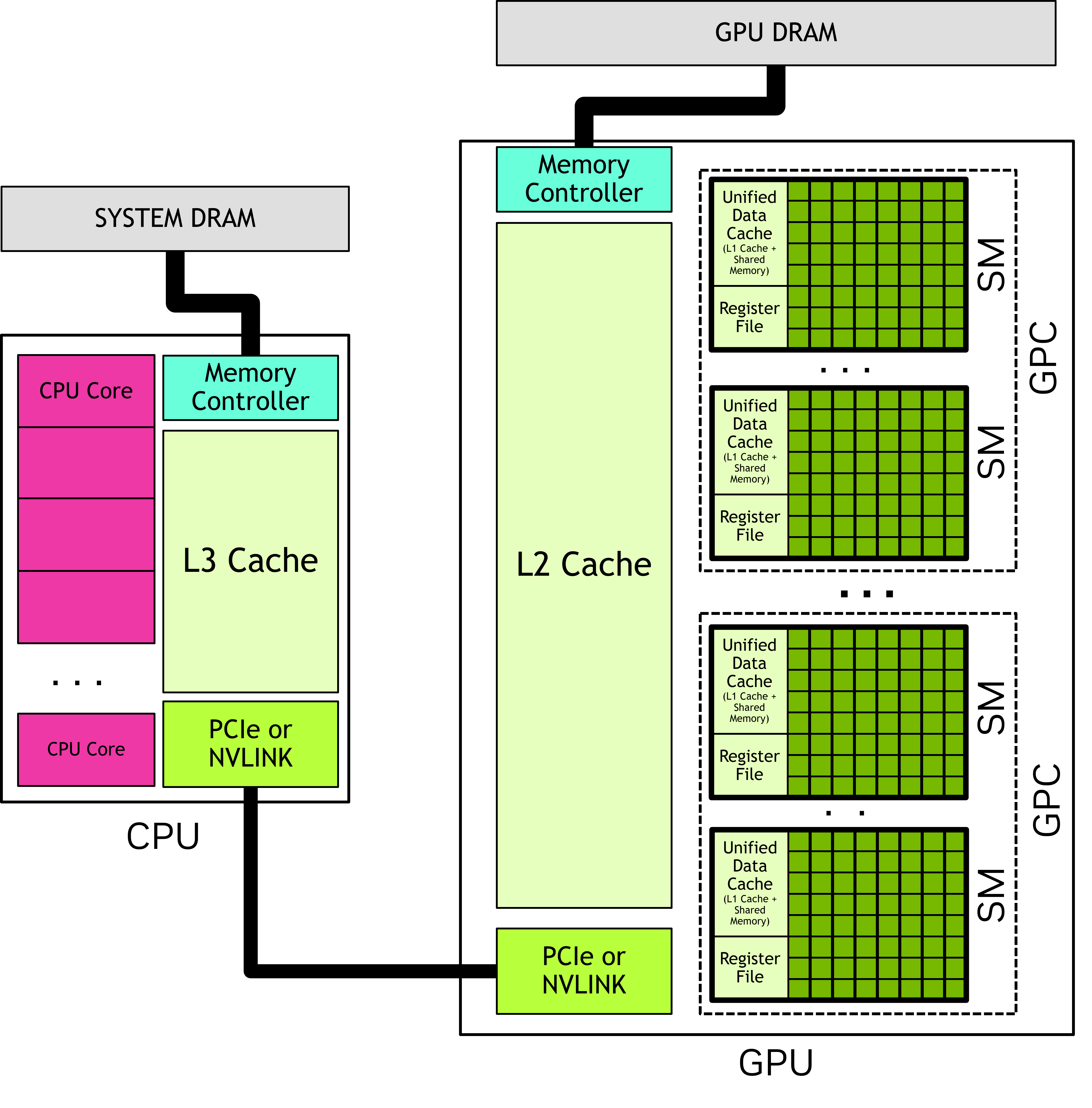
Source: NVIDIA, CUDA Programming Guide, Programming Model, Figure 2. The figure is a programming model, not a promise that every GPU generation has the same physical layout. Reproduced for technical commentary; rights remain with NVIDIA.

What this article owns

M4.2 owns:

host and device execution
kernel launch
grid, block, warp, and lane
SM residency and occupancy
register, shared-memory, cache, and HBM boundaries
global-memory coalescing
GEMM tiling
fusion and materialization
roofline reasoning
profiler evidence

It does not own:

online softmax and FlashAttention-1 exactness       -> M4.3
FlashAttention-2 work partitioning                  -> M4.4
split-KV decode, paged reads, and backend dispatch  -> M4.5
Hopper/Blackwell asynchronous attention pipelines  -> M4.6
KV allocation, reuse, scheduling, and placement     -> M5

The article is CUDA-facing because the local source and FlashAttention lineage are CUDA/GPU systems. The reasoning pattern still applies to other accelerators: identify the work hierarchy, local storage, global storage, movement path, synchronization model, and measured bottleneck.

0x01 Immutable Execution Contract And Source-To-Kernel Coordinates

The article keeps four claim classes separate.

Class	Meaning
Primary-source fact	Directly documented by NVIDIA or a cited paper.
Derived	Follows from an equation and stated assumptions in this article.
Illustrative	Uses hypothetical hardware numbers to expose the calculation.
Measured	Would require a named GPU, software stack, shape, dtype, and profiler output.

No local GPU benchmark is claimed in this article. Numerical roofline and occupancy examples are analytical illustrations unless a source and device are named.

Freeze the case before calculating it

M4.1 froze architecture, workload, numerical state, ownership, and accounting before deriving logical cost. M4.2 extends that manifest with the coordinates that turn logical cost into a physical execution hypothesis:

operation:
    semantic equation
    input/output shapes, strides, layouts, and aliases
    storage dtype and accumulation dtype
    training, prefill, or decode phase
    mask, dropout, causal, and numerical-reference contract

dispatch:
    framework and compiler versions
    eager, compiled, graph-captured, or library route
    requested and selected backend
    kernel symbol and fallback reason
    launch count, stream, and synchronization edges

machine:
    GPU model and compute capability
    SM count and warp size
    resident thread, warp, block, register, and shared-memory limits
    dtype/instruction-specific compute roof
    L1, L2, and DRAM bandwidth boundaries
    clocks, power policy, and concurrency

schedule:
    grid and block dimensions
    tile sizes, stage count, and warp roles
    tensor-axis ownership and address map
    registers per thread and shared memory per block
    materialized intermediates and synchronization protocol

observation:
    warmup and raw timing samples
    event/synchronization method
    backend diagnostic and kernel trace
    compiler resource report and profiler version
    exact metric names and replay mode
    output tolerance/error and raw artifact locator

Changing any coordinate creates a new case. In particular, an autotuner that selects a different tile or a compiler that emits a different kernel has not merely changed a footnote: it has changed the physical schedule being compared.

The manifest also separates three evidence labels:

analytical:
    equations evaluated from the declared operation, machine, and schedule

source-reported:
    a paper or official document result retained with its original conditions

locally measured:
    synchronized timing and profiler artifacts from the declared environment

unmeasured is a valid state. It is better than filling an observation record with analytical numbers and calling them measurements.

Corrections inherited from A18

The source article says that a block “occupies one SM.” The precise contract is:

one thread block executes on one SM at a time
one thread block does not span multiple SMs
one SM may host multiple resident blocks concurrently
the resident count is limited by threads, warps, registers,
shared memory, architectural block limits, and allocation granularity

The CUDA Programming Guide explicitly illustrates multiple active thread blocks on each SM.

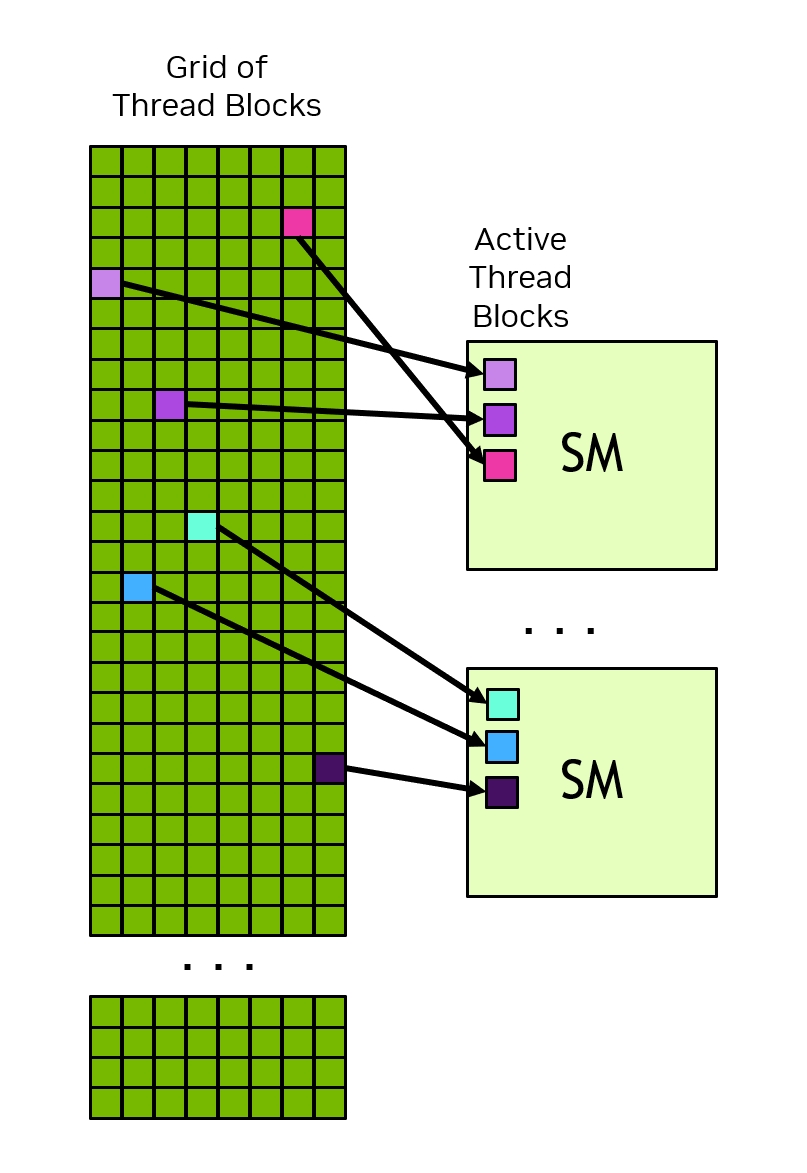
Source: NVIDIA, CUDA Programming Guide, Figure 4. A block remains on one SM, but a one-block-per-SM rule does not exist. Reproduced for technical commentary; rights remain with NVIDIA.

Other guardrails:

• “SRAM” is too broad for implementation reasoning. Registers, shared memory, and cache are different resources with different ownership and compiler control.
• High occupancy is not the same as high utilization or high performance.
• Peak tensor-core FLOP/s is not the throughput ceiling for every dtype, shape, instruction mix, or kernel.
• Theoretical HBM bandwidth is not the number of useful bytes delivered to a kernel.
• A tensor that exists in the mathematical graph need not be written to HBM.
• A fused kernel is not automatically faster if fusion causes spills, poor occupancy, redundant work, or an unfavorable schedule.

0x02 From A Framework Call To A Kernel Launch

Consider a PyTorch expression:

y = torch.nn.functional.silu(x @ weight)

The line is not a GPU execution specification. Depending on shape, dtype, device, compilation mode, library versions, and graph capture, it may produce:

one GEMM library kernel + one SiLU kernel
one GEMM kernel with an epilogue activation
a compiler-generated fused kernel
a fallback path
several setup, copy, or conversion kernels

The framework launches work from the host. A kernel launch supplies at least:

kernel function
grid dimensions
thread-block dimensions
dynamic shared-memory bytes
stream
kernel arguments

A simplified CUDA launch looks like:

dim3 grid(num_blocks_x, num_blocks_y, num_blocks_z);
dim3 block(threads_x, threads_y, threads_z);

kernel<<<grid, block, dynamic_smem_bytes, stream>>>(arguments...);

A source-to-kernel trace

The smallest publishable trace preserves every identity transition:

semantic source:
    y = silu(x @ W)

framework graph:
    aten::mm -> aten::silu

dispatch decision:
    eager library path, compiler fusion, or fallback

selected implementation:
    library algorithm / generated kernel / custom extension revision

kernel launch:
    symbol, grid, block, dynamic SMEM, stream, arguments

compiled resource record:
    registers/thread, static+dynamic SMEM, spill loads/stores, code target

runtime observation:
    ordered trace, synchronized duration, output error, profiler report

The middle of this chain is not stable across shapes. A large aligned GEMM may use a tensor-core library kernel; a small or irregular shape may select another algorithm; a compiler may fuse the activation into the epilogue; and an unsupported dtype or stride may fall back. The Python expression alone proves none of these outcomes.

The launch is asynchronous with respect to the host in the common case. The CPU can enqueue work and continue. Therefore this timing pattern is wrong:

start = time.perf_counter()
y = gpu_function(x)
elapsed = time.perf_counter() - start  # often measures enqueue time

A basic synchronized timing pattern is:

for _ in range(20):
    gpu_function(x)  # warm up compilation, caches, and allocations

torch.cuda.synchronize()

start = torch.cuda.Event(enable_timing=True)
end = torch.cuda.Event(enable_timing=True)

start.record()
for _ in range(100):
    gpu_function(x)
end.record()

torch.cuda.synchronize()
milliseconds = start.elapsed_time(end) / 100

This is still not a complete benchmark. The harness must also freeze:

GPU model and clocks
driver and CUDA versions
framework and backend versions
shape and stride
dtype and accumulation dtype
training/eval mode
causal/dropout/mask configuration
warmup and repetition policy
concurrency and stream state

Raw samples matter because one aggregate hides warmup, clock transitions, autotuning, interference, and tails. A minimal report keeps the samples and derives median, dispersion, and a tail quantile from the same immutable case.

Streams define order, not just concurrency

Operations enqueued in one CUDA stream execute in stream order. Different streams may overlap when dependencies and device resources permit; an event can make one stream wait for work in another. A host call returning only proves that work was enqueued, not completed.

host thread:  enqueue K0 ---- enqueue K1 ---- continue
stream 0:               [ K0 device work ][ K1 device work ]
event time:              ^ start                    end ^

CUDA Graph capture can reduce repeated host launch overhead by replaying a captured graph. It does not make an underfilled kernel compute-bound or repair bad memory access. It changes the launch path and therefore belongs in the dispatch manifest, not in a generic claim that graphs make kernels faster.

Launch count is a cost, but not the only cost

Launching many tiny kernels creates host/runtime overhead and intermediate materialization boundaries. Combining them can help. But one large kernel can become slower if it has too little parallel work or consumes too many registers and shared-memory bytes.

The optimization question is not:

Can these operators be fused?

It is:

Does the fused schedule reduce costly movement and launch overhead without creating a worse resource or parallelism bottleneck?

0x03 Grid, Block, Warp, And Lane Ownership

CUDA organizes a kernel launch into a grid of thread blocks. A block contains threads. Hardware groups the block’s threads into warps of 32 lanes.

Object	Scope	What it owns
grid	one kernel launch	all blocks for that launch
thread block / CTA	scheduled on one SM	a cooperating set of threads and block-local shared memory
warp	32 lanes from one block	an instruction-issue group under SIMT
thread / lane	one logical lane	indices, registers, and per-thread control state

Blocks may be scheduled in any order. Ordinary blocks cannot assume another block has run or can participate in a global barrier inside the kernel. Threads within one block can coordinate through block-scoped synchronization and shared memory.

Mapping data to work

A kernel usually maps block and thread indices to tensor coordinates:

int row = blockIdx.y * blockDim.y + threadIdx.y;
int col = blockIdx.x * blockDim.x + threadIdx.x;

For a matrix operation, a block may own an output tile rather than one scalar:

block (i, j)
    owns C[i : i+B_M, j : j+B_N]

warps inside the block
    own subtiles or pipeline roles

lanes inside each warp
    own fragments, loads, reductions, or stores

This ownership map is the bridge from tensor shape to parallel work. A shape can be large while the useful launch grid is small. During one-token decode, for example, the query-row axis may have length one, removing an axis that exposed many independent blocks during prefill.

Minimal tile and address trace

For C[M,N] = A[M,K] @ B[K,N], let a block own C[m0:m0+B_M, n0:n0+B_N]. The launch grid is:

$$G_M=\left\lceil\frac{M}{B_M}\right\rceil, \qquad G_N=\left\lceil\frac{N}{B_N}\right\rceil, \qquad G=G_MG_N$$

A flattened program id can be decoded as:

pid_m = pid // G_N
pid_n = pid % G_N
m0 = pid_m * B_M
n0 = pid_n * B_N

Inside one reduction stage k0, a lane does not load an abstract A tile. It computes an address from strides:

a_offset = (m0 + local_m) * stride_am + (k0 + local_k) * stride_ak
b_offset = (k0 + local_k) * stride_bk + (n0 + local_n) * stride_bn

a_valid = (m0 + local_m < M) and (k0 + local_k < K)
b_valid = (k0 + local_k < K) and (n0 + local_n < N)

The validity masks protect edge tiles. They do not remove all issued work: fixed-size tensor-core fragments or block-level schedules can still execute on partly empty tiles. The tiling analysis in 0x07 therefore accounts for useful versus issued tile work.

Triton expresses comparable ownership with program ids and block pointers; CUDA exposes blocks, threads, and explicit pointers; a vendor library hides most choices behind a selected algorithm. These are alternative programming surfaces over the same physical questions, not interchangeable source code.

Warps and divergence

All lanes in a warp execute the same instruction stream, with inactive lanes masked when control flow diverges. If half the lanes take one branch and half take another, the warp may execute both paths with different active masks.

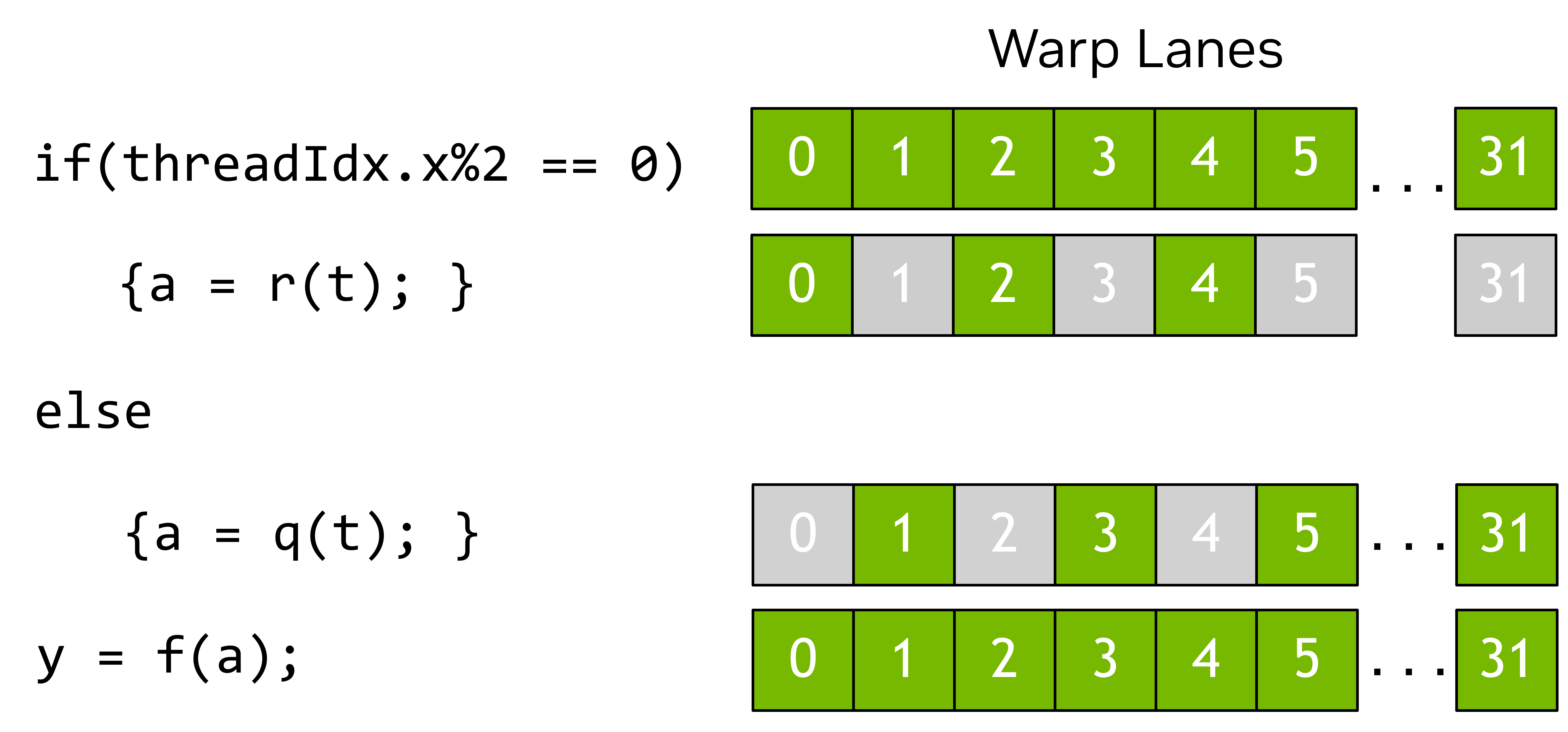
Source: NVIDIA, CUDA Programming Guide, Figure 7. Hardware details vary, but the SIMT contract explains why coherent control flow matters. Reproduced for technical commentary; rights remain with NVIDIA.

Divergence is not automatically the dominant bottleneck. A branch that skips a large amount of work may be valuable. The correct question is whether the branch creates enough inactive-lane execution to matter in the measured kernel.

0x04 SM Residency And Occupancy

An SM has finite resources. A block can become resident only if all required resources fit. A first-order resident-block model is:

$$N_{blocks}^{resident} = \min\left( N_{blocks}^{arch}, \left\lfloor\frac{T_{SM}}{T_{block}}\right\rfloor, \left\lfloor\frac{W_{SM}}{\lceil T_{block}/W_{size}\rceil}\right\rfloor, \left\lfloor\frac{R_{SM}}{R_{thread}T_{block}}\right\rfloor, \left\lfloor\frac{S_{SM}}{S_{block}}\right\rfloor \right)$$

where:

T_SM       maximum resident threads per SM
T_block    threads per block
W_SM       maximum resident warps per SM
W_size     hardware warp width
R_SM       32-bit registers available per SM
R_thread   registers allocated per thread
S_SM       shared-memory capacity available per SM
S_block    shared-memory bytes allocated per block
N_arch     architectural maximum resident blocks per SM

Real residency calculation rounds register and shared-memory allocations to architecture-specific granularities and can include named-barrier, cluster, or other generation-specific limits. Optional shared-memory/L1 partitioning can also change the available budget. The equation is a debugging model, not a replacement for the occupancy calculator and compiled-kernel report for the declared target.

The active-warp count is approximately:

$$W_{active} = N_{blocks}^{resident} \left\lceil\frac{T_{block}}{32}\right\rceil$$

and occupancy is:

$$\text{occupancy} = \frac{W_{active}}{W_{SM}^{max}}$$

Worked residency example

Use an illustrative SM budget:

maximum resident threads   T_SM   = 2048
maximum resident warps     W_SM   = 64
registers per SM           R_SM   = 65536
shared memory per SM       S_SM   = 164 KiB
architectural block limit          = 32

kernel block size          T_block  = 256 threads = 8 warps
registers per thread       R_thread = 64
shared memory per block    S_block  = 48 KiB

Each limit permits:

$$\begin{aligned} N_{threads} &= \left\lfloor\frac{2048}{256}\right\rfloor = 8 \\ N_{registers} &= \left\lfloor\frac{65536}{64\cdot256}\right\rfloor = 4 \\ N_{shared} &= \left\lfloor\frac{164}{48}\right\rfloor = 3 \\ N_{arch} &= 32 \end{aligned}$$

Shared memory is the first-order limiter, so three blocks may be resident:

$$W_{active} = 3\cdot8 = 24$$ $$\text{occupancy} = \frac{24}{64} = 37.5\%$$

If the block’s shared-memory allocation falls from 48 KiB to 32 KiB, the shared-memory ceiling rises to five blocks, but registers still limit the result to four:

$$N_{blocks}^{resident}=4, \qquad \text{occupancy}=\frac{4\cdot8}{64}=50\%$$

This does not prove the second kernel is faster. The shared-memory reduction may cause extra HBM traffic or recomputation. Conversely, the first kernel may have enough instruction-level parallelism and active warps to hide its important stalls.

Residency is a sensitivity surface

The same block can move between limiters when one schedule coordinate changes:

Change from the worked case	Thread ceiling	Register ceiling	Shared ceiling	First-order resident blocks
256 threads, 64 registers, 48 KiB	8	4	3	3
shared memory falls to 32 KiB	8	4	5	4
registers rise to 96/thread	8	2	3	2
block falls to 128 threads, same per-block SMEM	16	8	3	3

The last row shows why reducing threads per block need not increase residency: another fixed per-block resource can remain limiting. Conversely, accepting lower occupancy can be rational when it buys more accumulator state, reuse, or instruction-level parallelism.

Spills add a second failure path. If the compiler cannot allocate all live thread-local values in registers, some values can be addressed through local memory. “Local” describes per-thread addressability, not an on-chip residence guarantee; spill traffic can travel through cache and device-memory paths.

Occupancy is not utilization

Occupancy answers:

How many warps can be resident relative to the architectural maximum?

It does not answer:

how many cycles issue useful instructions
how busy tensor cores are
how much HBM bandwidth is achieved
how many lanes are active
whether warps are stalled on dependencies
whether the launch grid has enough blocks for all SMs

NVIDIA’s best-practices guidance is explicit: higher occupancy does not always produce higher performance, though low occupancy reduces the ability to hide latency. The useful profiler chain is:

theoretical residency
    -> achieved occupancy
    -> eligible warps
    -> issued warps
    -> stall reasons
    -> compute and memory throughput

Nsight’s scheduler vocabulary makes the causal gap explicit:

theoretical warps:
    allowed by the launch and resource model

active warps:
    resident and not yet completed

eligible warps:
    active and ready to issue an instruction now

issued warps:
    selected by a scheduler this cycle

High theoretical occupancy with few eligible warps points toward dependency or latency-hiding problems. High issued activity with low useful-lane work may instead indicate divergence or tail masks. Neither symptom is captured by one occupancy percentage.

0x05 Memory Hierarchy Means Ownership And Lifetime

A memory hierarchy diagram is useful only if it answers four questions:

who can access this state?
how long does it live?
who controls placement?
what traffic occurs when it is missed or spilled?

Resource	Typical scope	Typical role	Main failure mode
registers	thread/lane	accumulators, pointers, local state	pressure reduces residency or spills to local memory
shared memory	thread block	cooperative tiles, reductions, data exchange	capacity limit, bank conflicts, synchronization
L1/data cache	SM	cache for local/global traffic	cache behavior is not a programmer-owned tile contract
L2 cache	device	shared cache across SM traffic	working-set and access-pattern misses
HBM/global memory	device	model weights, activations, K/V, outputs	bandwidth, latency, transaction waste, materialization
host memory	CPU/system	input, output, offload, staging	interconnect transfer and synchronization

The FlashAttention paper’s motivating memory figure made the capacity/bandwidth asymmetry visible using A100-era values:

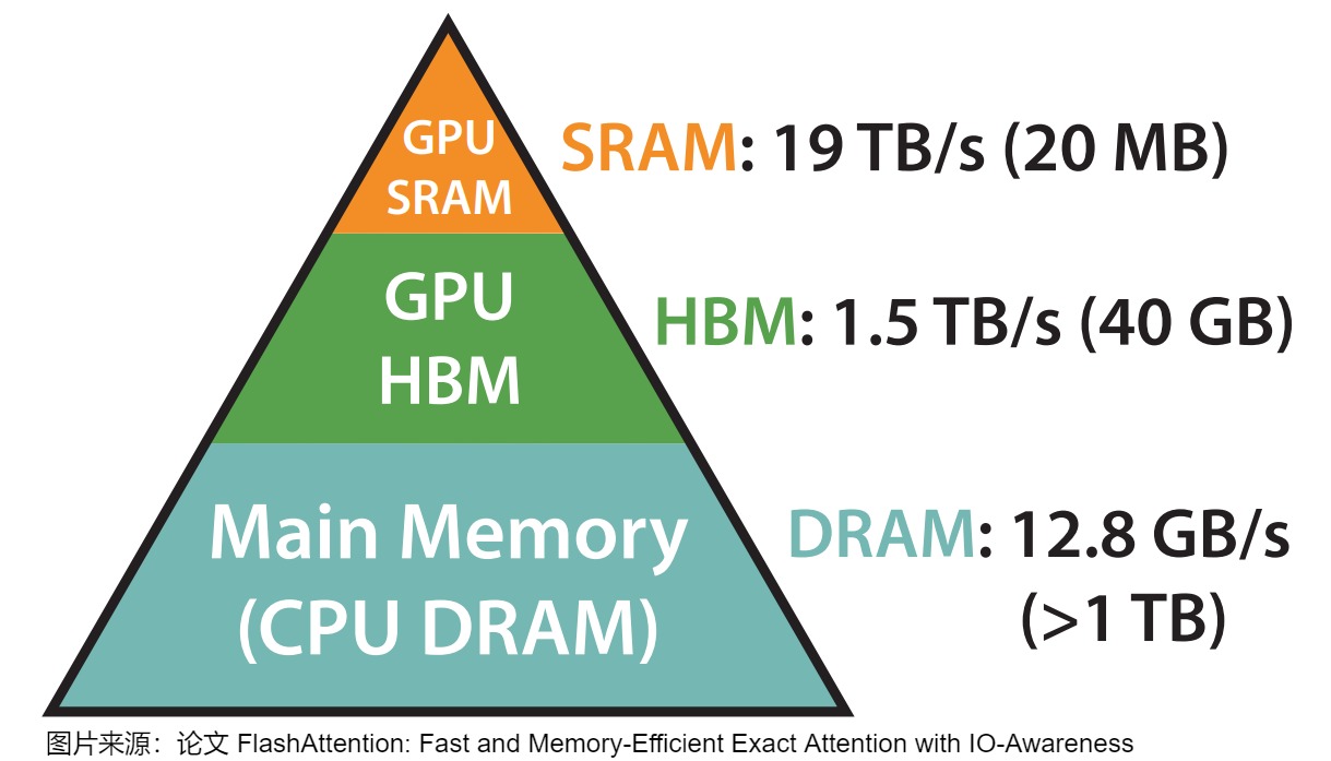
Source: FlashAttention, Figure 1, reused from A18. The numbers are hardware-specific; the durable claim is the large capacity/bandwidth difference between off-chip and on-chip storage. Reproduced for technical commentary; rights remain with the authors or publisher.

Registers are not a free private cache

Registers are low-latency thread state allocated by the compiler. A large accumulator or many live pointers can increase registers per thread. Since all resident threads share the finite register file, register use can reduce resident blocks.

If the compiler cannot keep required local state in registers, it may use local memory. Despite the name, local memory is off-chip addressable storage and can incur traffic through the cache/global-memory path. Compiler output and profiler evidence are needed to detect spills.

Shared memory is explicit but block-scoped

Shared memory is allocated per block. It is useful when threads cooperate on a tile, reuse data, transpose a layout, or perform a reduction. Its benefits come with constraints:

capacity limits resident blocks
loads and stores must avoid harmful bank conflicts
producer and consumer threads need correct synchronization
the lifetime ends with the block

Shared memory does not let ordinary independent blocks communicate. That would violate the block scheduling model.

Cache hits change measured traffic, not the logical ledger

M4.1 can calculate requested bytes. Actual DRAM traffic may be lower because data hits in L2, or higher because transactions fetch unused sectors, writebacks occur, or an implementation materializes additional workspaces.

Keep three byte ledgers separate:

logical bytes:
    elements required by the tensor algorithm

requested/effective bytes:
    useful bytes requested or produced by the kernel

actual traffic:
    sectors and bytes moved through L1/L2/DRAM interfaces

For profiling and Roofline reconciliation, use the full boundary chain:

logical tensor bytes
    -> requested useful bytes from active lanes
    -> sectors/transactions at the requesting cache
    -> L1-to-L2 traffic after L1 hits and evictions
    -> L2-to-DRAM traffic after L2 hits and evictions
    -> writebacks, atomics, and implementation workspaces

0x06 Coalescing: Layout Becomes Transactions

A warp does not issue 32 unrelated ideal scalar memory transfers. Hardware combines lane requests into memory transactions. On current CUDA guidance for compute capability 6.0 or higher, concurrent accesses are serviced by the number of 32-byte transactions needed to cover the requested addresses.

For 32 lanes loading adjacent FP32 values:

$$32\text{ lanes}\cdot4\text{ bytes}=128\text{ useful bytes}$$

With proper alignment, those addresses occupy four 32-byte sectors.

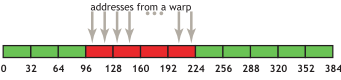
Source: NVIDIA, CUDA C++ Best Practices Guide, Coalesced Access, Figure 3. The exact transaction rules depend on compute capability. Reproduced for technical commentary; rights remain with NVIDIA.

For adjacent BF16 values:

$$32\cdot2=64\text{ useful bytes}$$

so an aligned access can fit in two 32-byte sectors.

Now suppose adjacent lanes load FP32 elements with stride two. The warp still requests 128 useful bytes, but the address span covers 256 bytes. A first-order sector count is eight, so only half of each fetched region is useful:

$$\text{load efficiency} \approx \frac{128}{8\cdot32} =50\%$$

Caches and reuse can modify measured DRAM traffic, but they do not make the access pattern coalesced.

The first-order sector calculation can be made executable. For addresses a_0,...,a_31, element width b, and sector width s, count the unique sectors touched by every byte interval:

$$N_{sector} = \left| \bigcup_{i=0}^{31} \left\{ \left\lfloor\frac{x}{s}\right\rfloor: x\in[a_i,a_i+b-1] \right\} \right|$$

Then the requested-to-sector efficiency is:

$$\eta_{sector} = \frac{N_{active}b}{N_{sector}s}$$

For 32 adjacent FP32 values aligned to a 32-byte sector boundary, N_sector=4 and eta_sector=1. Moving the first address by four bytes spans five sectors, so the same 128 useful bytes have a first-order efficiency of 128/160=80%. A neighboring warp may reuse the over-fetched sector from cache, which is why this is a request-boundary result rather than a DRAM-byte claim.

Transformer layout example

Suppose K is stored as:

K: [B, H_kv, T, d_h]

with d_h contiguous. Mapping neighboring lanes to neighboring head dimensions gives unit-stride loads inside one token/head row.

lane 0  -> K[b,h,t,0]
lane 1  -> K[b,h,t,1]
...
lane 31 -> K[b,h,t,31]

Mapping neighboring lanes across tokens instead can create a stride of d_h elements:

lane 0  -> K[b,h,t+0,d]
lane 1  -> K[b,h,t+1,d]
...

Whether that is harmful depends on the full layout and vectorization strategy. The point is that a shape such as [B,H,T,d_h] is insufficient. A kernel contract needs:

strides
alignment
vector width
lane-to-index mapping
page/block layout if K/V is non-contiguous

This becomes central in M4.5 and M5 when decode kernels traverse paged KV state.

Shared-memory banks are a second address map

Coalescing global loads does not guarantee conflict-free shared-memory access. For a common 32-bank, 32-bit-word model, a word address maps approximately as:

$$bank(word)=word\bmod32$$

Suppose a 32 x 32 FP32 tile is stored row-major. A warp reading one row touches successive banks. A warp reading one column at fixed column c touches word addresses 32r+c; every lane maps to bank c, creating a 32-way conflict in the simple model. Padding the row to 33 words changes the column addresses to 33r+c, distributing successive lanes across banks.

unpadded column: bank((32*r)+c) = c
padded column:   bank((33*r)+c) = (r+c) mod 32

The exact bank width, multicast behavior, and instruction mapping are architecture-specific. The invariant is that global layout, shared layout, and lane ownership must be audited separately.

0x07 Tiling: Reuse Data Before Eviction

Matrix multiplication is the canonical tiling example:

$$C_{M\times N}=A_{M\times K}B_{K\times N}$$

A block can own an output tile C_tile: [B_M,B_N], then iterate across the reduction dimension in chunks B_K:

for k0 in range(0, K, B_K):
    load A[M tile, K tile]
    load B[K tile, N tile]
    accumulate C tile
store C tile

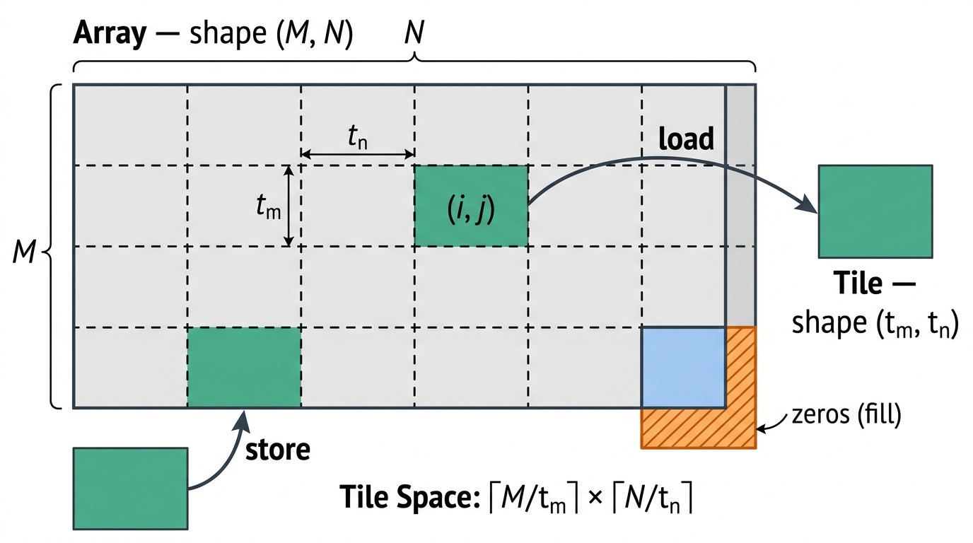
Source: NVIDIA, CUDA Programming Guide, Tile Space and Data Movement, Figure 9. A block is an execution unit; a tile is a data unit. They are related by the implementation, not identical by definition. Reproduced for technical commentary; rights remain with NVIDIA.

Per-stage arithmetic intensity

For one reduction stage, the block loads approximately:

$$E_{load}=B_MB_K+B_KB_N$$

elements and performs:

$$F_{stage}=2B_MB_NB_K$$

FLOPs under the multiply-add-equals-two convention.

If each input element occupies b bytes, the input-side stage intensity is:

$$I_{stage} \approx \frac{2B_MB_NB_K} {b(B_MB_K+B_KB_N)} = \frac{2B_MB_N}{b(B_M+B_N)}$$

For square 128 x 128 output tiles and BF16 inputs (b=2):

$$I_{stage} = \frac{2\cdot128\cdot128}{2(128+128)} =64\text{ FLOP/byte}$$

For 64 x 64 tiles:

$$I_{stage}=32\text{ FLOP/byte}$$

Larger tiles can increase reuse, but they also increase accumulator state, shared-memory demand, register pressure, edge waste, and sometimes synchronization.

Tile capacity example

Assume:

B_M = 128
B_N = 128
B_K = 32
input bytes b = 2
two shared-memory stages for double buffering

Staging A and B tiles requires approximately:

$$S_{staging} = 2\cdot b\cdot B_K(B_M+B_N)$$ $$=2\cdot2\cdot32(128+128) =32768\text{ bytes} =32\text{ KiB}$$

The FP32 accumulator tile contains:

$$128\cdot128\cdot4=65536\text{ bytes}=64\text{ KiB}$$

distributed across thread registers or other architecture-specific fragments. It is not one contiguous block-local array that can be assigned freely without resource consequences.

Tile-edge quantization

The grid rounds M and N up to whole output tiles:

$$M_{issued}=\left\lceil\frac{M}{B_M}\right\rceil B_M, \qquad N_{issued}=\left\lceil\frac{N}{B_N}\right\rceil B_N$$

A first-order output-tile utilization is:

$$\eta_{tile}=\frac{MN}{M_{issued}N_{issued}}$$

For M=N=129 with 128 x 128 tiles, the logical output has 16,641 elements, but the four-tile rectangle covers 65,536 positions:

$$\eta_{tile}=\frac{129^2}{256^2}\approx25.39\%$$

Masks prevent invalid memory accesses. They do not imply that all fixed tile instructions disappear. Library heuristics may choose a narrower tile to trade reuse for less edge waste.

Wave quantization

Let G be the number of launched blocks and let the first-order concurrent block slots be:

$$G_{wave}=N_{SM}N_{blocks}^{resident}$$

Then:

$$N_{waves}=\left\lceil\frac{G}{G_{wave}}\right\rceil$$

and, when the last wave is non-empty, its slot fill is:

$$\eta_{tail} = \frac{G-(N_{waves}-1)G_{wave}}{G_{wave}}$$

For 1,024 blocks, 108 SMs, and three resident blocks per SM, one wave has 324 slots. Four waves are needed, and the final wave contains only 52 blocks:

$$\eta_{tail}=\frac{52}{324}\approx16.05\%$$

This does not say the last wave lasts exactly as long as a full wave; block durations and overlap vary. It exposes a parallelism cliff that FLOP count does not contain.

Double buffering trades capacity for overlap

With one stage:

load tile
wait
compute tile
load next tile
wait
compute next tile

With a legal asynchronous pipeline:

compute stage 0 while loading stage 1
compute stage 1 while loading stage 0 for the next iteration

This can hide movement latency, but the extra stage consumes storage. The CUDA Best Practices Guide notes that asynchronous global-to-shared copies can avoid an intermediate register and overlap copy with computation on supported hardware. M4.6 revisits this idea with Hopper TMA/WGMMA pipelines, Blackwell TMEM/2-CTA execution, and explicit register/shared-memory tradeoffs.

0x08 Fusion: Remove A Materialization Boundary

Suppose two operators are executed separately:

kernel A:
    read X
    compute Z
    write Z to HBM

kernel B:
    read Z from HBM
    compute Y
    write Y

If one fused kernel can consume Z on chip, it can remove at least one HBM write and one HBM read of the intermediate:

$$Q_{saved}\approx2\cdot|Z|\cdot b_Z$$

Worked fusion lower bound

Let:

Z shape = [4096, 4096]
dtype   = BF16 = 2 bytes

Then:

$$|Z|\cdot b_Z =4096^2\cdot2 =33{,}554{,}432\text{ bytes} =32\text{ MiB}$$

The eliminated write-read round trip is 64 MiB. On an illustrative 1.5 TB/s memory interface, even the ideal bandwidth-only lower bound is:

$$t_{saved}^{ideal} = \frac{67{,}108{,}864}{1.5\cdot10^{12}} \approx44.7\ \mu s$$

This is not a runtime prediction. It ignores cache behavior, launch overhead, overlap, transaction waste, the rest of both kernels, and the fused kernel’s resource changes. It only shows that a logical intermediate can represent a meaningful physical round trip.

Why fusion can lose

Fusion may increase:

register live ranges
shared-memory allocation
instruction-cache pressure
synchronization
recomputation
compile time
tail waste for irregular shapes

If extra register pressure reduces residency or spills to local memory, the fused plan can lose the traffic it intended to save. Fusion is an execution hypothesis that needs measurement.

Alternative schedules move different bottlenecks

One operation can admit several legal schedules:

Schedule	Main gain	New cost or risk	Evidence required
larger output tile	more A/B reuse	fewer blocks, larger accumulator, edge waste	selected tile, registers, SMEM, waves
smaller output tile	more blocks and less edge waste	less reuse and repeated loads	traffic and achieved throughput
grouped tile order	better L2 reuse between neighboring CTAs	shape-dependent ordering and tails	L2 traffic/hit evidence
split-K	parallelism when M/N are small and K is large	partial-output reduction, workspace, atomics	reduction kernel and extra bytes
persistent CTAs	amortized setup and controlled reuse	fewer CTAs, load balance, long live state	waves, tile queue, registers, SMEM
extra pipeline stage	movement/compute overlap	more SMEM/registers, lower residency	async-copy and scheduler evidence
operator fusion	removes launch and materialization	longer live ranges, spills, less parallelism	kernel identity, spills, bytes, timing

Vendor libraries and Triton autotuners explore parts of this schedule space. The winning configuration is conditional on shape, dtype, layout, hardware, compiler, and concurrent workload. Autotuning results are therefore part of the dispatch/schedule manifest, not timeless properties of an operator.

0x09 Roofline: A Bound, Not A Runtime Oracle

Let:

F       useful floating-point operations
Q       bytes moved through the chosen memory boundary
C_peak  peak compute throughput
B_peak  peak bandwidth through that boundary
I       arithmetic intensity = F / Q

The simple roofline bound is:

Start from two independent lower bounds for a chosen work convention and memory boundary:

$$t_{compute}\ge\frac{F}{C_{peak}}, \qquad t_{memory}\ge\frac{Q}{B_{peak}}$$

If arithmetic and movement can overlap ideally, neither lower bound can be violated, so:

$$t\ge\max(t_{compute},t_{memory})$$

Since achieved performance is P=F/t and intensity is I=F/Q:

$$P \le \min\left( C_{peak}, B_{peak}\frac{F}{Q} \right)$$ $$P\le\min(C_{peak}, B_{peak}I)$$

The ridge point is:

$$I_{ridge}=\frac{C_{peak}}{B_{peak}}$$

A related lower bound on time is:

$$t\ge\max\left( \frac{F}{C_{peak}}, \frac{Q}{B_{peak}} \right)$$

The max is a lower-bound assumption, not a statement that every kernel perfectly overlaps all movement and computation. A strictly serialized schedule can approach a sum instead. Dependencies, barriers, issue limits, launch latency, and insufficient parallelism add constraints that the simple two-roof model does not represent.

Use an illustrative accelerator:

C_peak = 300 TFLOP/s
B_peak = 1.5 TB/s

Then:

$$I_{ridge} = \frac{300\cdot10^{12}}{1.5\cdot10^{12}} =200\text{ FLOP/byte}$$

A kernel with I=40 FLOP/byte has a bandwidth roof of:

$$B_{peak}I =1.5\cdot10^{12}\cdot40 =60\text{ TFLOP/s}$$

even though the compute peak is 300 TFLOP/s.

A kernel with I=400 FLOP/byte has a nominal bandwidth roof of 600 TFLOP/s, so the compute roof of 300 TFLOP/s becomes lower.

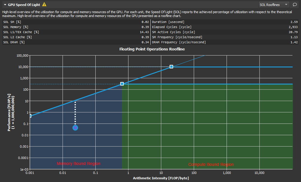
Source: NVIDIA, Nsight Compute Profiling Guide, Roofline Analysis. Hierarchical rooflines can expose L1, L2, and device-memory ceilings rather than treating “memory” as one level. Reproduced for technical commentary; rights remain with NVIDIA.

Worked time bound

Suppose a kernel performs:

F = 120 GFLOP
Q = 3 GB through HBM

On the illustrative accelerator:

$$t_{compute}^{min} = \frac{120\cdot10^9}{300\cdot10^{12}} =0.4\text{ ms}$$ $$t_{memory}^{min} = \frac{3\cdot10^9}{1.5\cdot10^{12}} =2.0\text{ ms}$$

The simple lower bound is 2.0 ms. A measured runtime of 3.2 ms would not prove that HBM alone is responsible. The gap can include limited parallelism, instruction throughput, dependency stalls, synchronization, launch overhead, cache behavior, or lower achieved bandwidth.

Choose the memory boundary explicitly

Arithmetic intensity changes depending on whether Q counts:

HBM traffic
L2 traffic
L1/shared-memory traffic
requested useful bytes
actual sectors transferred

This is why hierarchical rooflines are valuable. A kernel can be below the HBM roof but limited by shared-memory throughput or instruction issue.

For levels j in a memory hierarchy, use a separate measured or modeled byte count and bandwidth:

$$I_j=\frac{F}{Q_j}, \qquad t\ge \max\left( \frac{F}{C_{peak}}, \frac{Q_{L1}}{B_{L1}}, \frac{Q_{L2}}{B_{L2}}, \frac{Q_{DRAM}}{B_{DRAM}} \right)$$

One kernel therefore has several horizontal coordinates, not one context-free arithmetic intensity. The compulsory operand bytes from M4.1 may be a useful starting point, but an Nsight point needs counter-defined traffic at the same boundary as its bandwidth ceiling.

Peak, empirical, and achieved ceilings

C_peak must match the executed dtype, accumulation, and instruction path. Marketing tensor-core throughput is not the correct roof for an FP32 CUDA-core kernel or a kernel dominated by reductions and exponentials. Likewise, theoretical DRAM pin bandwidth and a sustained copy benchmark answer different questions.

Use three labels:

theoretical peak:
    architecture/vendor limit under stated clocks and instruction path

empirical machine ceiling:
    sustained result from a versioned characterization benchmark

achieved application point:
    work, traffic, and elapsed time measured for the target kernel

The distance from an achieved point to a roof is optimization headroom under that model. It is not causal proof. A high-intensity point far below the compute roof can be underfilled, instruction-latency limited, synchronization limited, or using a different instruction mix than the chosen roof.

0x0A Transformer Operations Under The Execution Model

M4.2 does not claim one bottleneck for every Transformer operation.

Operation	Typical physical pressure	Shape change that matters
large prefill GEMM	tensor-core work, tile reuse, staging	large M/N/K expose many blocks and reuse
one-row decode projection	weight reads, launch overhead, small-M schedule	M collapses toward active-token count
RMSNorm / LayerNorm	reductions and low arithmetic intensity	row width and number of rows
activation / elementwise	memory traffic and launch boundaries	total element count
prefill attention	score/probability materialization, softmax state, query tiles	both query and key lengths are large
decode attention	persistent K/V reads and limited query parallelism	q_len is one or small; k_len grows
output head	vocabulary-width GEMM and selection path	number of projected rows and vocabulary size

GEMM compulsory-byte contract

For C[M,N] = A[M,K] @ B[K,N], the useful arithmetic under the FMA-equals-two convention is:

$$F_{gemm}=2MKN$$

If each operand is read once and the output is written once at a chosen boundary, a compulsory-byte lower bound is:

$$Q_{gemm}^{min} = b_A MK+b_B KN+b_C MN$$

and:

$$I_{gemm}^{min-boundary} = \frac{2MKN}{b_A MK+b_B KN+b_C MN}$$

This is not a transaction prediction. It assumes perfect reuse inside the chosen boundary and excludes epilogues, partial-output reductions, workspaces, write-allocate effects, and cache refetches.

For BF16 inputs/output and a square projection with K=N=4096:

Row count M	Useful FLOPs	Compulsory bytes	First-order intensity
1	33,554,432	33,570,816	0.9995 FLOP/byte
128	4,294,967,296	35,651,584	120.47 FLOP/byte
4096	137,438,953,472	100,663,296	1,365.33 FLOP/byte

The weights dominate the one-row case and are amortized across many rows in prefill. The formulas do not guarantee those bytes come from DRAM: cache state, batching, and implementation decide the physical boundary.

Elementwise and reduction contracts

For a pointwise map y_i=f(x_i) with c_f useful operations per element and one input read plus one output write of b bytes:

$$I_{pointwise}^{min-boundary} = \frac{c_f}{2b}$$

Fusion can remove the input read or output materialization at one boundary, but may lengthen live ranges. A normalization also reduces across a row, usually requiring row statistics, synchronization, and more than one logical pass unless fused or reorganized. Quoting one universal FLOP/byte value for RMSNorm or LayerNorm would silently choose an implementation.

Example: prefill and decode can select different kernels

prefill Q: [B, H_q, S, d_h]
prefill K: [B, H_kv, S, d_h]

decode Q:  [B, H_q, 1, d_h]
cache K:   [B, H_kv, T, d_h]

The mathematical attention contract still contains QK^T, softmax, and PV. The work grid is not the same:

prefill:
    many independent query tiles
    substantial matrix-multiply work

decode:
    query-row axis collapses
    long cache must be read
    parallelism may move to heads, requests, or KV splits

M4.4 and M4.5 will use this execution model to distinguish FA2 query-block parallelism from split-KV decode.

Example: logical GQA savings require a physical grouped path

GQA reduces stored K/V heads:

Q heads:  H_q
KV heads: H_kv < H_q

The cache-byte ledger improves only if the runtime preserves the smaller K/V object. Materializing repeated K/V heads can reintroduce traffic. A grouped kernel can map multiple query-head groups to shared K/V loads without physically expanding the cache.

This is an execution boundary, not merely a shape annotation.

The operation atlas is a hypothesis table

The table and formulas justify candidate bottlenecks, not universal labels. “Transformer inference is memory-bound” is too coarse: a large prefill GEMM, a one-row projection, a fused normalization, and long-context decode attention can occupy different regions of the same GPU during one request.

0x0B Profiler Evidence: From Hypothesis To Trace

A performance explanation should move through an evidence ladder.

Level 1: tensor contract

Record:

shape
stride
dtype
device
mask/dropout/causal flags
training or inference

Level 2: analytical ledger

Estimate:

FLOPs
useful bytes
materialized intermediates
launch count
expected work-grid axes
first-order residency limits

Level 3: backend and kernel identity

Verify:

which framework backend was selected
which kernels launched
whether fallback occurred
whether a logical fusion actually became one kernel

Level 4: measured runtime

Use warmup, device events, synchronization, repeated shapes, and distribution statistics. Report median and a tail statistic rather than one timing.

Level 5: hardware counters

Inspect at least:

Question	Profiler evidence
Is the launch grid large enough?	grid dimensions, waves per SM, tail effects
What limits residency?	registers, shared memory, blocks, warps
Are warps issuing?	active, eligible, and issued warps; skipped issue slots
Is memory busy?	DRAM/L2/L1 throughput and transaction efficiency
Is compute busy?	tensor/core pipeline throughput and instruction mix
Are loads useful?	requested versus actual bytes, sectors, cache hit rates
Did registers spill?	local-memory loads/stores and compiler resource report
Is control flow coherent?	branch efficiency and active-lane behavior

NVIDIA Nsight Compute defines occupancy as active warps divided by possible active warps and warns that higher occupancy does not always mean higher performance. Its scheduler statistics distinguish active, eligible, and issued warps. That is more informative than quoting occupancy alone.

A broad collection command is:

ncu --set full -o m4_2_report python benchmark.py

The exact sections and metric names vary by Nsight Compute release and GPU architecture. A publishable experiment records both.

Profiler sections answer different questions. LaunchStats establishes launch shape and static resources; Occupancy compares theoretical and achieved residency; SchedulerStats distinguishes active, eligible, and issued warps; MemoryWorkloadAnalysis exposes cache and DRAM traffic; and ComputeWorkloadAnalysis reports pipeline activity. A high percentage in one section is not a complete bottleneck diagnosis.

Metric collection can require replay and can perturb cache state or elapsed time. The report must record profiler version, section set, replay mode, kernel filter, and whether timing came from the unprofiled benchmark or the profiled run. Timing and counters are related evidence, not automatically the same run.

Minimal result schema

hardware:
    GPU model
    compute capability
    clock policy
    memory capacity/bandwidth reference

software:
    driver
    CUDA
    framework
    compiler/backend

input:
    shapes
    strides
    dtype
    flags

launch:
    kernel name
    grid
    block
    registers/thread
    shared memory/block

result:
    median runtime
    achieved compute throughput
    achieved memory throughput
    achieved occupancy
    limiting residency resource
    dominant stall evidence
    numerical error against reference

Without this schema, “the kernel is memory-bound” is often an untested interpretation.

Executable Evidence Bundle: Empty Is Different From Measured

The repository now contains a machine-checked version of this schema:

docs/numinens-evidence/m4-m5-p1/kernel_bundle_template.json
docs/numinens-evidence/m4-m5-p1/validate_kernel_bundle.py

The checked-in bundle is deliberately labeled unmeasured. The validator allows an empty template, but a locally_measured result is rejected unless it contains at least 20 raw timing samples, the exact dispatch key, selected backend, kernel symbol, reference tolerances and errors, profiler command, profiler report, and hardware counters. This prevents two common evidence failures:

timing without kernel identity
    -> a fast fallback can be mistaken for the intended implementation

profiler counters without a numerical reference
    -> a fast but incorrect kernel can be presented as an optimization

Run the schema check with:

python3 docs/numinens-evidence/m4-m5-p1/validate_kernel_bundle.py \
  docs/numinens-evidence/m4-m5-p1/kernel_bundle_template.json

The current artifact validates as an empty evidence record, not as a GPU result. No CUDA measurement was produced during this content pass. NVIDIA’s Nsight Compute CLI supports saved reports, kernel filters, selected metric sets, and CSV output; the exact command and metric names must therefore remain inside the result bundle rather than being implied by prose.

0x0C Executable Estimator And Predicted-Observed Reconciliation

The article’s analytical path is executable in:

docs/numinens-evidence/m4-2-gpu-execution-model/
    execution_manifest.json
    gpu_execution_estimator.py
    observation_unmeasured.json
    test_gpu_execution_estimator.py

The manifest freezes the operation, illustrative machine, schedule, warp request, fusion boundary, and hierarchical Roofline case. It deliberately does not name a real GPU. The estimator derives the same quantities as the prose:

grid and issued tile extent
resource-limited resident blocks and occupancy
concurrent block slots, wave count, and tail fill
requested bytes, sector count, and sector efficiency
stage FLOPs, bytes, and arithmetic intensity
compulsory GEMM bytes and fusion round-trip bytes
L1, L2, and DRAM Roofline lower bounds

Run it with:

python3 docs/numinens-evidence/m4-2-gpu-execution-model/gpu_execution_estimator.py \
  docs/numinens-evidence/m4-2-gpu-execution-model/execution_manifest.json \
  --observation docs/numinens-evidence/m4-2-gpu-execution-model/observation_unmeasured.json \
  --fail-on-mismatch

The exact checked fixture closes at:

Derived object	Exact result
32 x 32 output-tile grid	1,024 blocks
resident blocks per SM	3, limited by shared memory
active warps and occupancy	24, 37.5%
concurrent block slots	324
waves and final-wave blocks	4, 52
final-wave slot fill	16.049382716049383%
aligned FP32 warp request	128 useful bytes, 4 sectors, 100% efficiency
128 x 128 x 32 tile stage	1,048,576 FLOPs, 16,384 bytes, 64 FLOP/byte
fused 4096 x 4096 BF16 round trip	67,108,864 bytes removed
hierarchical Roofline lower bound	0.002 seconds

The observation file returns:

status: unmeasured
observed median: absent
predicted lower bound: 0.002 seconds
residual: absent

This distinction is part of the result, not missing paperwork. When a valid measurement exists, reconciliation is:

$$r_t=t_{observed,median}-t_{predicted,lower-bound}$$

A nonnegative residual is expected because the analytical number is a lower bound. It must be explained with observed launch, issue, traffic, occupancy, spill, synchronization, or dispatch evidence. The code rejects an incomplete locally_measured label, fewer than 20 raw samples, a case-id mismatch, or a kernel whose numerical error exceeds its declared tolerance.

Run the rejection and sensitivity suite with:

python3 docs/numinens-evidence/m4-2-gpu-execution-model/test_gpu_execution_estimator.py

0x0D Failure Lab

Execution-model failures

1. Treating one framework call as one kernel. Compilation and dispatch may fuse, split, or fall back.

2. Treating a block as an SM. A block stays on one SM, but an SM can host multiple blocks and execute many blocks over time.

3. Assuming blocks execute in grid order. Ordinary blocks cannot depend on that schedule.

4. Confusing block and tile. A block is an execution unit; a tile is a data unit chosen by the implementation.

5. Assuming every thread maps to one CUDA core permanently. Threads are scheduled in warps over functional pipelines; the mapping is not a dedicated-core ownership contract.

Resource failures

6. Using too many registers. Residency falls or state spills to local memory.

7. Calling local memory on-chip. CUDA local memory is thread-scoped in address semantics but physically off-chip/cache-backed.

8. Increasing shared memory without recalculating residency. Better reuse can reduce the number of resident blocks.

9. Equating occupancy with utilization. Resident warps can still be stalled or inactive.

10. Maximizing occupancy at any cost. Forcing fewer registers can create spills or destroy useful instruction-level parallelism.

11. Ignoring allocation granularity. The simple floor equations can overestimate real residency.

Memory and layout failures

12. Counting useful elements as actual transactions. Misalignment, stride, and sector fetches can move extra bytes.

13. Assuming cache hits from one benchmark generalize. Batch, sequence, concurrency, and cache state change reuse.

14. Using a coalesced global layout that creates shared-memory bank conflicts. Optimization at one memory level can expose another bottleneck.

15. Materializing a logical broadcast. expand-style semantics can become a physical copy through reshape, fallback, or kernel choice.

16. Ignoring page/block layout in decode. Logical K/V continuity does not imply contiguous physical addresses.

Tiling and fusion failures

17. Choosing the largest tile that fits. It may leave too few blocks, waste edges, or create excessive accumulator pressure.

18. Double buffering without including both stages in the shared-memory ledger.

19. Missing synchronization between shared-memory producers and consumers. Results can be nondeterministically wrong.

20. Assuming fusion always reduces runtime. Fusion can spill, reduce parallelism, or duplicate work.

21. Confusing no HBM materialization with no intermediate state. The state still exists logically and may occupy registers/shared memory.

Roofline and measurement failures

22. Using peak FLOP/s for the wrong dtype or instruction path.

23. Using theoretical bandwidth as achieved useful bandwidth.

24. Computing arithmetic intensity without naming the memory boundary.

25. Timing asynchronous enqueue work with a CPU timer.

26. Benchmarking the first invocation. Compilation, autotuning, allocation, and cold caches contaminate the result.

27. Profiling one shape and generalizing to all Transformer phases.

28. Reading one high-level utilization number without work-grid and stall evidence.

29. Ignoring profiler replay overhead or clock variability.

30. Claiming a backend from the API name. Dispatch must be observed.

31. Treating masked edge positions as zero issued work. Predication protects correctness but fixed tile instructions and tail CTAs can remain.

32. Ignoring wave quantization. A small tail wave can leave most concurrent block slots empty.

33. Using one arithmetic intensity for every cache level. L1, L2, and DRAM traffic are different denominators.

34. Treating a Roofline distance as causal proof. The point can be below a roof because of issue, parallelism, synchronization, or a mismatched ceiling.

35. Calling an analytical fixture measured. A measured label requires raw timing, dispatch, profiler, and numerical artifacts.

0x0E Publish-Gate Checks

The article-level gate records where each requirement is established. It does not claim that a local GPU benchmark was run; measured claims remain explicitly out of scope unless a versioned result artifact is attached.

Gate	Status
the physical runtime problem appears before CUDA taxonomy	0x00
operation, dispatch, machine, schedule, and observation are immutable coordinates	0x01
logical tensor objects are separated from physical allocations	0x02, 0x05
host launch and asynchronous timing semantics are explicit	0x02
API, backend, and kernel identities remain separate	0x02, 0x0B
grid, block, warp, and lane ownership are correct	0x03
one tile and lane-address trace is executable from strides	0x03
one-block-per-SM language has been removed	0x04
registers, shared memory, L1, L2, and HBM are not collapsed into “SRAM”	0x05
occupancy includes its limiting resource and is not called utilization	0x04
active, eligible, and issued warps are distinct	0x04, 0x0B
tile sizes include register/shared-memory consequences	0x07
tile-edge and wave quantization are derived	0x07
coalescing claims name dtype, alignment, stride, and hardware scope	0x06
shared-memory banks have a separate address audit	0x06
fusion claims include removed bytes and new resource cost	0x08
split-K, persistent, buffering, and tile alternatives are compared	0x08
roofline equations name the counted memory boundary	0x09
theoretical, empirical, and achieved ceilings are distinguished	0x09
Transformer bottlenecks are operation- and phase-specific	0x0A
measured-claim schema names hardware, software, shape, dtype, and flags	0x0B
kernel/backend identity has an evidence procedure	0x0B
numerical parity against a reference is required	0x0B
exact synthetic estimator fixtures close without becoming measurements	0x0C
predicted lower bound, observation, and residual are separate	0x0C

0x0F Handoff To M4.3

M4.2 has established the physical vocabulary needed for IO-aware attention:

HBM materialization is an execution choice
tiles create local reuse
blocks own work tiles
warps execute and cooperate inside blocks
register/shared-memory demand limits residency
layout determines transactions
fusion trades movement for resource pressure
roofline gives a bound
profilers decide which hypothesis survived execution

The next article can now ask a narrower algorithmic question:

Softmax couples every key in a query row through one denominator. How can an attention kernel stream K/V tiles, keep only compact row state on chip, and still return exactly the same normalized result?

M4.3 - IO-Aware Attention and FlashAttention-1 owns that proof and algorithm.

The boundary is strict:

M4.1 owns:
    logical work, state, and compulsory-byte schedules

M4.2 owns:
    generic GPU schedule realization, machine ceilings, and profiler evidence

M4.3 owns:
    online-softmax state, exact FA1 recurrence, tile loop, and IO proof

M4.4-M4.6 own:
    attention-version work partition, decode reduction, and new hardware pipelines

M5 owns:
    request-level K/V lifecycle, paging, scheduling, reuse, and placement

M8 owns:
    numerical formats, quantizer metadata, packing, and quantized release

0xFE Claim Status And Scope

Claim family	Status	Scope
CUDA hierarchy, streams, coalescing, shared-memory banks	externally anchored	current official CUDA documentation; architecture qualifications retained
occupancy and Nsight evidence ladder	externally anchored	current Nsight Compute concepts; metric names remain version-specific
tile/wave quantization alternatives	externally anchored and derived	NVIDIA GEMM guide plus article formulas
Roofline and hierarchical boundaries	externally anchored and derived	original and hierarchical Roofline sources
exact fixture numbers	rewrite interpretation, synthetic-contract tested	illustrative manifest; no named hardware result
A18 motivation and A100 hierarchy	source-local, corrected and scoped	historical context, not a current hardware specification
kernel timing or profiler conclusion	unmeasured	no local CUDA artifact was produced

0xFF References

Local series

• M4.1 - Transformer Cost Model
• A18 - Exploring the Transformer Series: FlashAttention
• M4.3 - IO-Aware Attention and FlashAttention-1
• M4.4 - FlashAttention-2 And Decoding Kernel Boundary
• M4.5 - Decode Kernels And Backend Boundaries
• M4.6 - FlashAttention Hardware Pipelines
• M5.1 - Autoregressive Serving State
• M8.1 - Quantized Numbers

Primary and official sources

• NVIDIA, CUDA Programming Guide, Programming Model
• NVIDIA, CUDA Programming Guide, Writing SIMT Kernels
• NVIDIA, CUDA Programming Guide, Writing Tile Kernels
• NVIDIA, CUDA C++ Best Practices Guide
• NVIDIA, Matrix Multiplication Background User’s Guide
• NVIDIA, GPU Performance Background User’s Guide
• NVIDIA, Nsight Compute Profiling Guide
• Williams, Waterman, and Patterson, Roofline: An Insightful Visual Performance Model for Multicore Architectures
• Yang et al., Hierarchical Roofline Performance Analysis for Deep Learning Applications
• PyTorch, CUDA Semantics
• Triton, Fused Softmax Tutorial
• Triton, Matrix Multiplication Tutorial
• Dao et al., FlashAttention: Fast and Memory-Efficient Exact Attention with IO-Awareness
• Dao, FlashAttention-2: Faster Attention with Better Parallelism and Work Partitioning