M3.7 — Residual Stream, Normalization, and Block Assembly

0x00 Overview And Background

M3.1 opened one attention call. M3.2 added projection, head layout, concatenation, and the output projection. M3.6 reconstructed the dense and gated MLP.

Those sublayers share an important output contract:

attention output: [B, S, d_model]
MLP output:       [B, S, d_model]

But a Transformer block is not merely:

attention -> MLP

Each sublayer updates a persistent state tensor through a residual branch, normalization, and sometimes dropout:

X_l: [B, S, d_model]
    -> attention branch update
    -> MLP branch update
X_{l+1}: [B, S, d_model]

M3.7 owns that block update. Its local questions are:

Which tensor is the residual state?
Where is normalization applied?
Which axis does normalization reduce?
Where does dropout sit relative to the residual add?
Does the checkpoint use Pre-LN, Post-LN, LayerNorm, or RMSNorm?
Is there a final normalization after the layer stack?

These choices often preserve every visible tensor shape. A shape-correct implementation can still be a different model.

Owner question

How can hundreds of nonlinear sublayers update one persistent state without erasing its identity or destabilizing scale, and exactly where do residual addition, normalization, dropout, and depth-dependent scaling sit?

M3.7 owns the derivation from residual learning to a full Transformer block, not only the final diagram. That includes identity and gradient paths across depth, LayerNorm/RMSNorm forward and backward geometry, normalization axes, Pre-LN/Post-LN optimization differences, final normalization, residual scaling, DeepNorm-style variants, and training/runtime fusion.

It defers the internal score and MLP functions to M3.1–M3.6, whole-model performance to M4, persistent request state to M5.1, multi-request scheduling to M5.2, and physical cache state to M5.3.

---

Background knowledge: deep stacks need an identity path and controlled scale

Residual connections came from deep vision networks as a way to let a layer learn a change to an existing representation rather than reconstruct the whole representation. Normalization controls activation scale and optimization behavior. Transformers combine both ideas around attention and MLP sublayers.

residual path:
    preserves a direct state and gradient route across depth

normalization:
    controls row-wise channel scale before or after a sublayer

dropout:
    regularizes the learned update branch during training

block assembly:
    fixes the exact order in which these operations interact

Pre-LN, Post-LN, LayerNorm, and RMSNorm are not interchangeable labels. Their placement and parameterization affect checkpoint compatibility, training stability, and the final normalization required before the output head.

Residual learning was introduced to solve degradation, not only vanishing gradients

The original ResNet observation was that making a network deeper could increase training error even when the added layers could, in principle, learn identity. This degradation is not the same claim as gradients numerically underflowing. Residual parameterization asks the branch to learn a correction:

$$y=x+F(x;\theta)$$

instead of asking a stack to reconstruct the full target mapping $H(x)$ directly. If the desired mapping is near identity, the branch can approach $F(x)=0$.

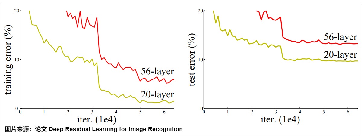
The vision result motivates the parameterization; it does not prove that every Transformer instability is solved by an unscaled skip connection. Transformer branches contain normalization, attention, MLPs, dropout, and depth-dependent initialization, so their combined dynamics need a separate contract.

The block did not arrive as one indivisible invention

The modern Transformer wrapper is easier to understand when its ingredients are kept in historical order.

1. Highway Networks learned gates that mixed a transformed path with a carry path. The carry route helped information cross depth, but its learned gate was itself part of the optimization problem.
2. Deep Residual Learning made the default shortcut an exact identity when shapes matched. Its key empirical problem was degradation: deeper plain networks could have higher training error, even though extra layers should be able to represent identity.
3. Identity Mappings in Deep Residual Networks separated the shortcut from branch and post-add transformations. This made the conditions for a clean forward and backward identity route explicit.
4. Layer Normalization introduced example-local normalization whose statistics do not depend on the other examples in a mini-batch. The exact reduction axes still depend on the tensor contract; Transformer LayerNorm later standardized each token row’s feature coordinates.
5. The original Transformer wrapped every attention and MLP sublayer with a residual add followed by LayerNorm. This is Post-LN, even though many pedagogical implementations later adopted Pre-LN wrappers.
6. Later systems changed different parts independently: Pre-LN moved the norm, RMSNorm removed mean subtraction, DeepNorm coupled residual scaling with initialization, and decoder-only families such as LLaMA used Pre-RMSNorm plus a final RMSNorm.

This chronology prevents a common category error. A residual connection is not a normalization method, and a normalization formula does not determine where it is placed. A complete block is the product of several independent choices:

block identity
    = branch graph
    + residual equation
    + normalizer family and axes
    + normalizer placement
    + branch stochasticity
    + depth parameterization
    + final-stack normalization

Two checkpoints can therefore contain tensors with the same shapes while implementing different functions.

Claim-status and terminology firewall

This article uses four evidence labels:

Label	Meaning here
Source-local	stated or illustrated in A2, A4, or A12-A14; not automatically treated as externally established
Primary-paper verified	supported by the named original paper under that paper’s architecture and experiment
Implementation verified	checked against a version- or commit-pinned official implementation
Derived contract	algebra, tensor ownership, or engineering consequence derived here and covered by a local oracle where practical

The vocabulary is fixed before the derivations begin:

Term	Exact meaning in M3.7	Not implied
residual state / stream	the persistent [B,S,d_model] state read and updated by block branches	a claim that semantic features occupy disjoint channels
shortcut / identity path	the route carrying a branch input to its residual add	that every architecture leaves this route unscaled or ungated
branch update	an attention, cross-attention, or MLP result after its declared scaling/dropout	a standalone new sequence state
normalization family	LayerNorm, RMSNorm, ScaleNorm, or another declared transform	its placement relative to branch and add
topology	the ordered operator graph, including final norm	merely the list of module class names
row	one x[b,s,:] feature vector unless another reduction group is stated	a whole sentence or a batch statistic

The term residual stream is an explanatory name for the state shared across depth. The original Transformer paper describes residual connections; it does not require this later interpretability vocabulary. M3.7 uses the term because it makes read/write ownership visible, not to claim that the stream is an architecturally separate memory tensor.

Article route and ownership firewall

The derivation proceeds from the persistent state outward:

identity and update algebra
    -> LayerNorm and RMSNorm geometry
    -> normalization placement and local Jacobians
    -> encoder / decoder / decoder-only block assembly
    -> dropout, saved state, recomputation, and dtype
    -> depth parameterization and paper variants
    -> fused and distributed runtime integration
    -> evaluation, release, and rollback

M3.1-M3.2 remain the owners of attention scores, masks, heads, and output projection. M3.6 remains the owner of dense and gated MLP internals. M3.7 may show those sublayers as black-box branch functions, but it owns only the wrapper that reads and updates the persistent model-width state.

0x01 The residual-stream shape contract

Let the input to layer l be:

X_l: [B, S, d_model]

A residual update has the form:

$$X_{l+1}=X_l+F_l(X_l)$$

The addition is elementwise, so both operands must have identical shapes:

identity path:  X_l       [B, S, d_model]
branch output:  F_l(X_l)  [B, S, d_model]
updated state:  X_{l+1}   [B, S, d_model]

The residual operation does not concatenate features, append rows, or average layers. It adds a branch update to the state already flowing through the stack.

For one block with attention and MLP branches:

X_l
  -> attention residual update -> X_attn
  -> MLP residual update       -> X_{l+1}

This model-width contract explains why M3.2 ends attention with an output projection and why M3.6 contracts d_ff back to d_model.

Residual is not automatic compatibility

Matching rank is insufficient:

[B,S,d_model] + [B,S,d_ff]       invalid width
[B,S,d_model] + [B,h,S,d_head]   unmerged heads
[B,T,d_model] + [B,S,d_model]    wrong row ownership

The branch must return the same semantic axes as the state it updates.

Unrolling the residual stream across depth

For a simplified stack

$$x_{l+1}=x_l+F_l(x_l),$$

repeated substitution gives

$$x_L=x_l+\sum_{i=l}^{L-1}F_i(x_i).$$

The state at depth $L$ is the earlier state plus accumulated updates. This additive expression is why the term residual stream is useful: branches read a common-width state and write corrections back into it.

The loss gradient with respect to $x_l$ is

$$\frac{\partial\mathcal L}{\partial x_l} =\frac{\partial\mathcal L}{\partial x_L} \left(I+\frac{\partial}{\partial x_l} \sum_{i=l}^{L-1}F_i(x_i) \right).$$

Equivalently, in local Jacobian product form,

$$\frac{\partial x_L}{\partial x_l} =\prod_{i=l}^{L-1}(I+J_{F_i}).$$

The identity term creates a direct additive route, but the product can still amplify or attenuate directions according to the branch Jacobians. “Residuals prevent vanishing gradients” is therefore an intuition, not an unconditional theorem.

Exact state expansion and ordered Jacobian product

Introduce explicit shortcut and branch coefficients:

$$x_{i+1}=a_i x_i+b_i u_i(x_i),$$

where u_i includes the branch’s declared norm, sublayer, and deterministic scale but excludes the shortcut. For ordinary Pre-LN, $a_i=b_i=1$ and $u_i(x_i)=F_i(N_i(x_i))$.

When every shortcut is identity, repeated substitution gives the exact finite-state telescoping equation already shown:

$$x_L=x_l+\sum_{i=l}^{L-1}u_i(x_i).$$

The branch values are evaluated at different states, so this is not a linear superposition of fixed functions of $x_l$. It supports an accounting statement — each layer writes an additive update — but not the claim that the network is linear.

With scaled shortcuts, the exact expansion becomes:

$$x_L=\left(\prod_{j=l}^{L-1}a_j\right)x_l +\sum_{i=l}^{L-1} \left(\prod_{j=i+1}^{L-1}a_j\right)b_i u_i(x_i).$$

Every update is multiplied by the shortcuts after it. Empty products equal one. This formula makes the clean identity contract concrete: when all $a_j=1$, neither the original state nor an earlier update is exponentially scaled merely by traversing later shortcuts.

The infinitesimal contract is different. Define $J_i=\partial u_i/\partial x_i$. With column-vector convention:

$$\frac{\partial x_L}{\partial x_l} =\left(a_{L-1}I+b_{L-1}J_{L-1}\right) \cdots \left(a_lI+b_lJ_l\right).$$

The order matters because Jacobians generally do not commute. One cannot multiply a list of per-layer eigenvalues unless the matrices share the necessary eigenvectors. Singular values provide norm bounds,

$$\left\|\frac{\partial x_L}{\partial x_l}\right\|_2 \le \prod_{i=l}^{L-1}\left\|a_iI+b_iJ_i\right\|_2,$$

but this upper bound can be loose. Stable training is a property of the full parameterization, data, optimizer, and evolving Jacobians, not the visible + operator alone.

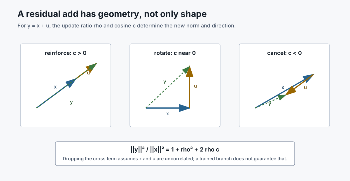
Update geometry: magnitude and alignment both matter

For one token row, write $y=x+u$. A useful local ledger records:

$$\rho=\frac{\|u\|_2}{\|x\|_2}, \qquad c=\frac{x^\top u}{\|x\|_2\|u\|_2}.$$

Then:

$$\frac{\|y\|_2^2}{\|x\|_2^2} =1+\rho^2+2\rho c.$$

The same update ratio can have different effects:

c near +1: update reinforces the current direction
c near  0: update adds an approximately orthogonal component
c near -1: update cancels part of the current state

Across a population of token rows, the second-moment identity is:

$$\mathbb E\|x+u\|_2^2 =\mathbb E\|x\|_2^2 +\mathbb E\|u\|_2^2 +2\mathbb E[x^\top u].$$

The cross term is why “variance grows by one branch variance per layer” is not generally valid. Attention/MLP updates are functions of the current state and can be strongly correlated with it. An independence assumption must be stated before dropping covariance.

What Pre-LN controls and what it leaves free

In Pre-LN,

$$x_{i+1}=x_i+F_i(N_i(x_i)),$$

the branch reads a normalized row, but the persistent stream after the add is not itself constrained to unit variance or fixed RMS. Its magnitude can grow, shrink, or rotate according to the accumulated, correlated updates. The next branch again receives a normalized view, and the stack-final norm reconciles the last residual state with the output-head input contract.

In Post-LN,

$$x_{i+1}=N_i(x_i+F_i(x_i)),$$

each stored layer output is normalized, but the local gradient to the previous state passes through $J_{N_i}$. “Normalized activations” and “clean identity gradient route” are therefore separate properties.

Residual hypotheses are evidence with scope

Residual connections have several non-exclusive explanations: easier identity parameterization, direct gradient terms, ensemble/path interpretations, and changes to optimization-landscape singularities. For example, Orhan and Pitkow’s Skip Connections Eliminate Singularities studies elimination, overlap, and linear-dependence singularities in simplified models and deep-network experiments. It is evidence for one optimization mechanism, not a proof that these are the only reason Transformer residuals work.

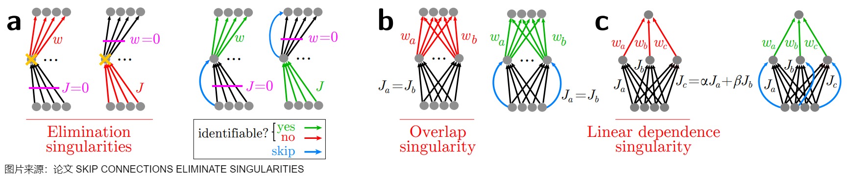
The practical M3.7 rule is narrower: preserve the declared identity/update graph, measure state and update geometry, and test the actual end-to-end Jacobian or gradients under the intended training recipe.

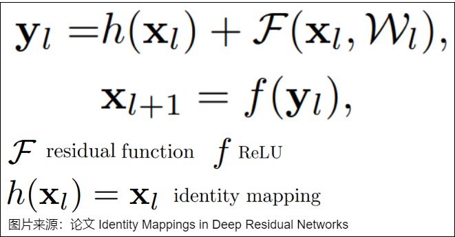
Why a clean identity shortcut matters

Consider a generalized update

$$x_{l+1}=h_l(x_l)+F_l(x_l).$$

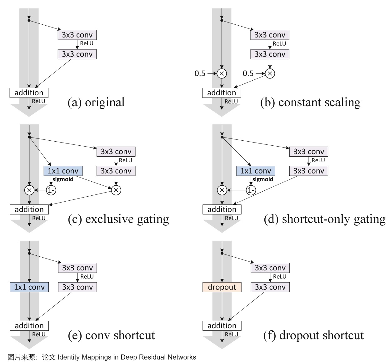
If $h_l(x)=\lambda_lx$, the direct path across depth is scaled by $\prod_l\lambda_l$. Values below one attenuate it; values above one amplify it. If $h_l$ is a learned projection or gate, the direct route also inherits its Jacobian and parameters.

The ResNet v2 analysis compares constant scaling, gates, projections, and dropout on shortcuts. For a Transformer whose branch already returns d_model, the ordinary shortcut is normally exact addition. A projection belongs only where state width or ownership genuinely changes.

Residual state is not a free semantic partition

Because every branch writes into the same vector space, one cannot generally point to disjoint slices and declare one “attention memory” and another “MLP memory.” The learned projections can rotate and superpose features across all channels. Residual-stream analysis should track directions, causal effects, and update magnitudes rather than assuming named modules own permanent channel ranges.

Immutable block identity: shape is only the first field

A runnable model needs a block manifest, not the label “Transformer layer.” M3.7 treats the following fields as architecture identity:

architecture_id: llama_style_pre_rmsnorm_decoder
state_layout: [batch, sequence, model]
branch_order: [causal_self_attention, gated_mlp]
norm:
  family: rmsnorm
  placement: pre_branch
  reduction_axes: [-1]
  epsilon: 1.0e-6
  center: false
  scale: per_channel
  bias: false
residual:
  shortcut_scale: 1.0
  attention_branch_scale: 1.0
  mlp_branch_scale: 1.0
dropout:
  attention_output: 0.0
  mlp_output: 0.0
final_norm: rmsnorm

That architectural record is joined to four more manifests:

Manifest	Fields that cannot be guessed from tensor rank
tensor	axis names, valid rows, dtype, device, stride/contiguity, branch owner
checkpoint	exact key, shape, transpose convention, tied/aliased state, norm bias presence, final norm
training	dropout probabilities and RNG identity, saved/recomputed tensors, initialization gains, optimizer state
runtime	eager/fused backend, accumulation dtype, residual dtype, parallel ownership, deterministic policy

Changing any architecture field changes the model function. Changing a runtime field may preserve the intended function but alter numerical error, saved state, or reproducibility. The distinction must be recorded rather than assumed.

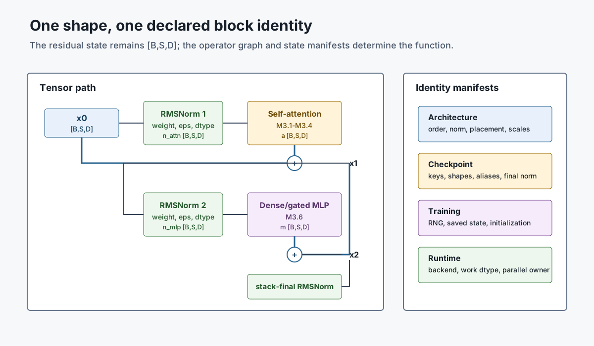
Source-to-tensor trace: one decoder block

For a LLaMA-style layer, let the source object be a contiguous hidden-state tensor and its validity/position metadata:

hidden_states x0: [B,S,D]
attention_mask:   broadcastable to the selected attention backend
position state:   coordinates or precomputed rotary embeddings owned by M3.4

M3.7 begins after those objects have been validated. The exact wrapper trace is:

Step	Tensor	Shape	State owner	Checkpoint/runtime dependency
0	x0	[B,S,D]	persistent residual state	input dtype/device/layout
1	r_attn = x0	[B,S,D]	identity route	alias or explicit handle, not a mathematical copy requirement
2	n_attn = norm_1(x0)	[B,S,D]	attention branch input	input_layernorm.weight, epsilon, accumulation dtype
3	a = attention(n_attn, ...)	[B,S,D]	branch update	M3.1-M3.4 plus output projection/backend
4	x1 = r_attn + scale_a * dropout_a(a)	[B,S,D]	new persistent state	residual/branch scale, dropout RNG
5	r_mlp = x1	[B,S,D]	identity route	alias/liveness policy
6	n_mlp = norm_2(x1)	[B,S,D]	MLP branch input	post_attention_layernorm.weight, epsilon, dtype
7	m = mlp(n_mlp)	[B,S,D]	branch update	M3.6 topology and weights
8	x2 = r_mlp + scale_m * dropout_m(m)	[B,S,D]	layer output state	branch scale, dropout RNG
9	z = final_norm(x_L)	[B,S,D]	stack output	final norm.weight, epsilon, output-head contract

The residual handles at steps 1 and 5 denote value ownership, not an instruction to allocate full copies. An eager implementation may keep Python references; a fused kernel may retain the residual in registers or a separate accumulation buffer. Any in-place update is legal only if backward and recomputation no longer need the overwritten value.

Checkpoint reconciliation is topology reconciliation

For a decoder layer numbered l, a common LLaMA checkpoint includes:

model.layers.l.input_layernorm.weight          [D]
model.layers.l.self_attn.*                     attention state
model.layers.l.post_attention_layernorm.weight [D]
model.layers.l.mlp.*                           MLP state
model.norm.weight                              [D]  # stack-final norm

The two per-layer norm keys do not identify Post-LN operations. Their meaning comes from call order in the model class. Likewise, absence of norm bias is an RMSNorm checkpoint fact, not permission to synthesize a zero bias and silently change the declared module family.

An import must reconcile:

expected key set == loaded key set after an explicit migration map
expected tensor shape == loaded tensor shape after a declared transpose only
expected norm family/epsilon/topology == architecture configuration
expected final norm == output-head input contract

strict=False is not architecture inference. It can hide a missing final norm, an accidentally shared LayerNorm, or a Post-LN checkpoint loaded into a Pre-LN graph while every remaining matrix still has a plausible shape.

---

0x02 LayerNorm normalizes channels inside each row

For Transformer states:

x: [B, S, d_model]

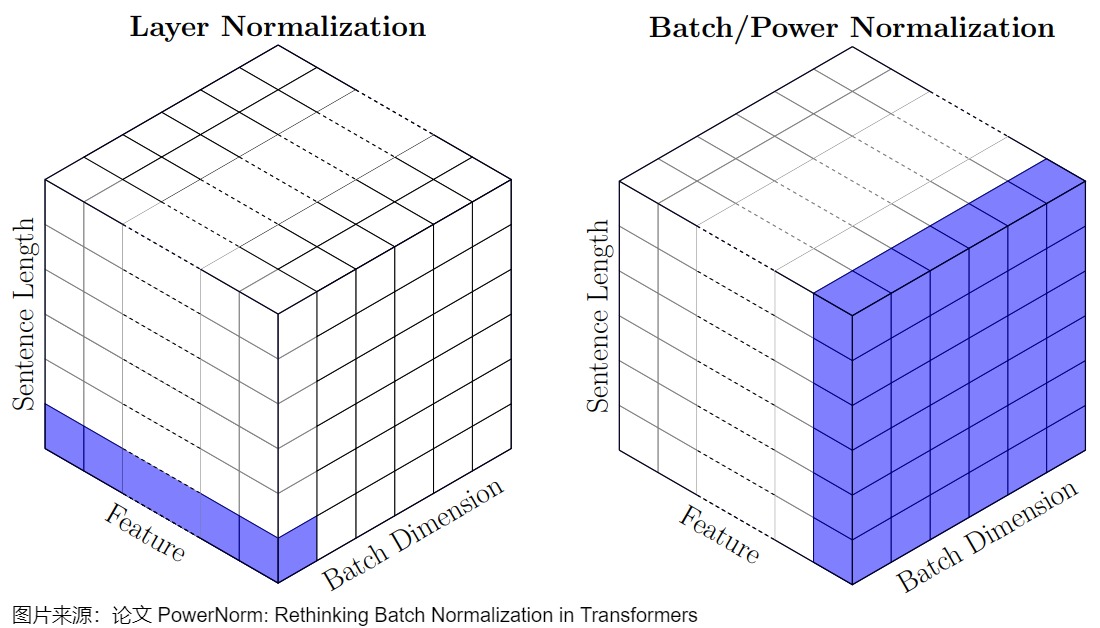
LayerNorm(d_model) computes statistics over the final feature axis independently for every (batch, sequence) row.

For row x[b,s,:]:

$$\mu_{b,s}=\frac{1}{d}\sum_{r=1}^{d}x_{b,s,r}$$ $$\sigma^2_{b,s}=\frac{1}{d}\sum_{r=1}^{d}(x_{b,s,r}-\mu_{b,s})^2$$ $$y_{b,s,r}=\gamma_r\frac{x_{b,s,r}-\mu_{b,s}} {\sqrt{\sigma^2_{b,s}+\epsilon}}+\beta_r$$

The shape trace is:

x:             [B, S, d_model]
mean:          [B, S, 1]
variance:      [B, S, 1]
gamma / beta:  [d_model]
y:             [B, S, d_model]

This is not normalization over the batch axis and not normalization over the sentence as one S * d_model vector. Each token row receives its own feature mean and variance.

An exact PyTorch-shaped reconstruction is:

def layer_norm_last_dim(x, weight, bias, eps=1e-5):
    # x: [B, S, d_model]
    mean = x.mean(dim=-1, keepdim=True)
    var = x.var(dim=-1, keepdim=True, correction=0)
    x_hat = (x - mean) * torch.rsqrt(var + eps)
    return x_hat * weight + bias

The PyTorch 2.13 torch.nn.LayerNorm contract uses the last dimensions named by normalized_shape, places epsilon inside the square root, and uses the biased variance estimator (correction=0).

Source-audit correction: the A14 educational class is approximate

A14 imports this educational implementation:

def forward(self, x):
    mean = x.mean(-1, keepdim=True)
    std = x.std(-1, keepdim=True)
    return self.a_2 * (x - mean) / (std + self.eps) + self.b_2

It correctly points at the last axis and preserves shape, but it is not numerically identical to nn.LayerNorm:

educational code:
    denominator = std + eps
    torch.std default correction may differ

PyTorch LayerNorm:
    denominator = sqrt(var(correction=0) + eps)

That distinction is technically small in prose and operationally important in checkpoint-compatible code. M3.7 uses the official formula as the implementation contract.

LayerNorm also does not perform the same operation as BatchNorm. BatchNorm derives statistics over batch-related axes and commonly tracks running statistics; Transformer LayerNorm operates per state row and uses current-row statistics in both training and evaluation.

LayerNorm geometry and invariances

Ignoring epsilon and affine parameters for the moment, define

$$\hat x=\frac{x-\mu\mathbf1}{\sigma}.$$

Its normalized row satisfies

$$\mathbf1^\top\hat x=0, \qquad \frac{1}{d}\|\hat x\|_2^2=1.$$

LayerNorm removes a component along the all-ones direction and rescales the centered vector to a fixed root-mean-square magnitude. For any positive scalar $a$ and scalar shift $c$,

$$\operatorname{LN}_0(ax+c\mathbf1)=\operatorname{LN}_0(x),$$

where LN_0 omits epsilon and learned affine parameters. Negative $a$ flips the normalized direction. Finite epsilon makes scale invariance approximate near very small variance.

The learned $\gamma$ and $\beta$ then restore per-channel scale and shift capacity:

$$y=\gamma\odot\hat x+\beta.$$

Deriving LayerNorm with a centering projector

For one row $x\in\mathbb R^d$, define the centering matrix:

$$C=I-\frac1d\mathbf1\mathbf1^\top.$$

It is symmetric and idempotent:

$$C^\top=C, \qquad C^2=C, \qquad C\mathbf1=0.$$

The centered row is $z=Cx=x-\mu\mathbf1$. The biased population variance used by the PyTorch LayerNorm contract is:

$$v=\frac1d z^\top z,$$

not the sample estimate with denominator $d-1$. Define $r=\sqrt{v+\epsilon}$. The non-affine transform is then:

$$\hat x=\frac{Cx}{\sqrt{\frac1d\|Cx\|_2^2+\epsilon}}.$$

This decomposition explains the geometry:

1. C projects away the all-ones shift direction.
2. division by r projects the centered row toward a sphere;
3. gamma scales coordinates and beta translates them again.

With $\epsilon=0$ and nonzero variance, $\hat x$ lies in a (d-1)-dimensional zero-mean hyperplane and has norm $\sqrt d$. The radial rescaling removes one additional local degree of freedom, so the non-affine Jacobian has rank at most d-2. Epsilon makes the radial direction weakly nonzero near the origin, while the constant-shift direction remains exactly null before affine parameters.

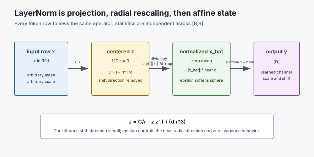
The exact non-affine Jacobian is:

$$J_{\hat x} =\frac1r C-\frac1{d r^3}zz^\top.$$

Multiplying on the left by $\operatorname{Diag}(\gamma)$ gives the Jacobian of the affine LayerNorm output. This form is also a direct route to the compact backward equation below.

Epsilon, variance, and accumulation dtype are architecture/runtime state

Four superficially small choices produce different functions:

Field	Required contract	Consequence of changing it
variance denominator	d / correction=0 for the cited PyTorch contract	d-1 rescales every normalized row, especially at small d
epsilon location	sqrt(variance + eps)	sqrt(variance) + eps has different units and behavior near zero variance
reduction axes	last dimensions named by normalized_shape	changing axes couples different tokens, samples, or feature groups
work dtype	backend-declared accumulation dtype	low precision can erase small deviations or corrupt moment subtraction

The one-pass identity

$$v=\mathbb E[x^2]-\mathbb E[x]^2$$

is exact over real numbers but can subtract two large, nearly equal floating-point values. A two-pass centered reduction or Welford-style online state avoids that specific cancellation pattern. Which algorithm is fastest and sufficiently accurate is a backend decision; M3.7’s correctness contract requires finite statistics and parity within a declared tolerance, not one mandatory kernel schedule.

For a constant row $x=c\mathbf1$:

$$z=0, \qquad \hat x=0, \qquad y=\beta.$$

The epsilon makes the denominator finite. The non-affine input Jacobian becomes $C/\sqrt\epsilon$; it is not an identity map, and for d=1, C=0, so the normalized output contains no input-dependent information. These edge cases belong in tests because production shapes usually hide them.

The official PyTorch 2.13 LayerNorm documentation fixes correction=0, places epsilon under the square root, uses input statistics in both training and evaluation, and gives learned affine state the full normalized_shape. Those are framework facts, not universal requirements for every normalization paper.

LayerNorm backward derivation

Let upstream gradient be $g_y=\partial\mathcal L/\partial y$ and define $g_{\hat x}=g_y\odot\gamma$. For one row with $r=\sqrt{\sigma^2+\epsilon}$, the input gradient is

$$g_x =\frac{1}{r}\left[ g_{\hat x} -\operatorname{mean}(g_{\hat x})\mathbf1 -\hat x\operatorname{mean}(g_{\hat x}\odot\hat x) \right].$$

The three terms have distinct roles:

g_hat:
    incoming channel gradient

- mean(g_hat):
    removes the component created through the row mean

- x_hat * mean(g_hat * x_hat):
    removes the component created through the row scale

Affine-parameter gradients reduce over all rows that share the norm parameters:

$$g_\gamma=\sum_{b,s}g_y[b,s,:]\odot\hat x[b,s,:], \qquad g_\beta=\sum_{b,s}g_y[b,s,:].$$

This backward equation is why a normalization kernel needs row-wise reductions in both directions, not just an elementwise divide.

An implementation-level backward trace for one [B,S,D] tensor is:

forward saved or recomputed:
    x or centered row z       [B,S,D]
    reciprocal std rstd      [B,S,1]
    gamma                     [D]

upstream:
    g_y                       [B,S,D]

row reductions:
    sum(g_y * gamma)          [B,S,1]
    sum(g_y * gamma * x_hat)  [B,S,1]

outputs:
    g_x                       [B,S,D]
    g_gamma                   [D]  reduction over B,S
    g_beta                    [D]  reduction over B,S

Saving mean and rstd is cheaper than saving another full activation, but the backward still needs either x, x_hat, or enough upstream state to recompute the centered row. Activation checkpointing may recompute those values; it must use the same epsilon, reduction axes, weights, and work-dtype policy.

Why BatchNorm is a different training and serving contract

For a feature channel, BatchNorm estimates moments across a mini-batch and possibly spatial/sequence axes:

$$\mu_B=\frac1m\sum_{i=1}^{m}x_i, \qquad \sigma_B^2=\frac1m\sum_{i=1}^{m}(x_i-\mu_B)^2.$$

Training outputs therefore depend on which examples and valid positions share the statistic. Variable sequence lengths require careful masking, microbatch size changes the estimate, and distributed training may need synchronized statistics. Inference commonly switches to running moments accumulated during training.

LayerNorm has none of those batch-state transitions: each token row carries all coordinates needed for its statistic. This makes it naturally compatible with batch size one and incremental decode. It does not mean BatchNorm is mathematically impossible in sequence models; PowerNorm, PRepBN, and related work explicitly explore alternatives, but they introduce different state and optimization assumptions.

Normalization axes are the method

For an activation tensor [B,S,D], saying only “normalize” is incomplete:

Method	Typical reduction group on [B,S,D]	Couples examples?	Couples token positions?	Inference state
LayerNorm	each (b,s,:) row	no	no	none beyond learned affine state
RMSNorm	each (b,s,:) row’s squared magnitude	no	no	none beyond learned scale
BatchNorm-style channel norm	selected (b,s) entries for each feature	yes	often yes	running moments in common designs
InstanceNorm adaptation	positions/features within one example, definition-dependent	no	often yes	usually no running batch moments
GroupNorm adaptation	groups of channels, possibly per row	no if row-local	depends on layout	learned affine state

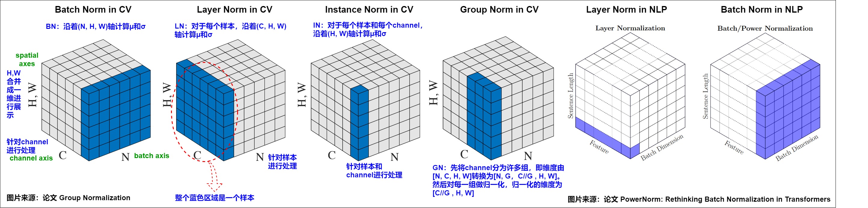
Padding makes coupled statistics especially delicate. If padded rows participate in a BatchNorm-like estimate, changing the batch’s sequence-length distribution changes valid-token outputs. Row-wise LayerNorm/RMSNorm still normalizes a padded row independently; a later attention or loss mask determines whether that row affects other computation.

Normalization is also distinct from masking:

mask:
    controls visibility, participation, or loss ownership

normalization:
    transforms values using a declared reduction group

A causal mask does not change LayerNorm’s feature-axis statistics, and LayerNorm does not prevent attention to future tokens.

---

0x03 RMSNorm keeps rescaling and removes re-centering

RMSNorm uses the root mean square without subtracting a row mean:

$$\operatorname{RMS}(x_{b,s})= \sqrt{\frac{1}{d}\sum_{r=1}^{d}x_{b,s,r}^{2}+\epsilon}$$ $$y_{b,s,r}=\gamma_r\frac{x_{b,s,r}} {\operatorname{RMS}(x_{b,s})}$$

The shape contract remains:

x:        [B, S, d_model]
mean(x²): [B, S, 1]
weight:   [d_model]
y:        [B, S, d_model]

Transformers v5.13.1 computes LLaMA RMSNorm in float32 and casts back to the input dtype:

class LlamaRMSNorm(nn.Module):
    def __init__(self, hidden_size, eps=1e-6):
        super().__init__()
        self.weight = nn.Parameter(torch.ones(hidden_size))
        self.variance_epsilon = eps

    def forward(self, hidden_states):
        input_dtype = hidden_states.dtype
        hidden_states = hidden_states.to(torch.float32)
        variance = hidden_states.pow(2).mean(-1, keepdim=True)
        hidden_states = hidden_states * torch.rsqrt(
            variance + self.variance_epsilon
        )
        return self.weight * hidden_states.to(input_dtype)

The RMSNorm paper argues that LayerNorm’s re-centering component is dispensable in the studied settings and proposes a computationally simpler rescaling operation. That supports a narrow statement:

LayerNorm:
    subtract mean, divide by standard deviation, apply affine parameters

RMSNorm:
    divide by root mean square, apply scale

It does not justify a universal claim that RMSNorm is always more stable or always produces better models.

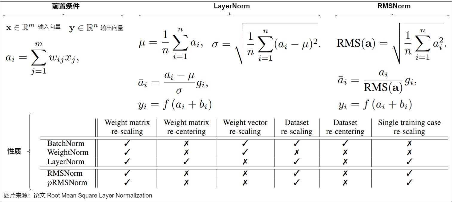
RMSNorm geometry and backward path

Let

$$r=\sqrt{\frac1d x^\top x+\epsilon}, \qquad \hat x=\frac{x}{r}.$$

Ignoring epsilon, $\|\hat x\|_2^2=d$. RMSNorm is invariant to positive scalar rescaling but not to adding a constant offset:

$$\operatorname{RMSNorm}_0(ax)=\operatorname{RMSNorm}_0(x), \qquad a>0,$$ $$\operatorname{RMSNorm}_0(x+c\mathbf1) \ne\operatorname{RMSNorm}_0(x) \quad\text{in general}.$$

With $g_{\hat x}=g_y\odot\gamma$, the row gradient is

$$g_x =\frac1r\left[ g_{\hat x} -\frac{\hat x}{d} (g_{\hat x}^\top\hat x) \right].$$

The second term removes the radial component induced by normalization. RMSNorm avoids the mean-related reduction in LayerNorm, but still requires a sum of squares and a dot-product-like backward reduction.

RMSNorm Jacobian and its exact relationship to LayerNorm

For one row, let:

$$q=\frac1d x^\top x, \qquad r=\sqrt{q+\epsilon}, \qquad \hat x=\frac{x}{r}.$$

The non-affine Jacobian is:

$$J_{\mathrm{RMS}} =\frac1r I-\frac1{d r^3}xx^\top.$$

This is the LayerNorm Jacobian without the centering projector. With $\epsilon=0$, the radial direction is null, while the all-ones shift direction is not generally null. RMSNorm therefore keeps positive rescaling invariance but not recentering invariance.

The two denominators satisfy:

$$\operatorname{RMS}(x)^2 =\operatorname{Var}(x)+\epsilon+\mu(x)^2.$$

For an exactly zero-mean row, non-affine LayerNorm and RMSNorm have the same denominator and output. For a nonzero-mean row they differ even if their weight, epsilon, and shape match. A useful diagnostic is therefore the ratio:

$$\frac{\operatorname{RMS}(x)}{\sqrt{\operatorname{Var}(x)+\epsilon}} =\sqrt{1+\frac{\mu(x)^2}{\operatorname{Var}(x)+\epsilon}}.$$

Large row means increase that divergence. It cannot be repaired by copying a LayerNorm scale vector into an RMSNorm module.

Partial RMSNorm is an estimator contract, not ordinary RMSNorm

The original RMSNorm paper also proposes partial RMSNorm (pRMSNorm). For a declared subset $\mathcal S$ of m coordinates:

$$\widehat{\operatorname{RMS}}_{\mathcal S}(x) =\sqrt{\frac1m\sum_{j\in\mathcal S}x_j^2+\epsilon},$$

and the whole row is divided by that estimate. With the full set, it recovers RMSNorm. With a strict subset, it preserves common positive rescaling but adds estimation error and makes subset selection part of the architecture/runtime contract:

subset coordinates or sampling rule
subset size / p value
whether the subset is fixed or resampled
distributed ownership of sampled coordinates
epsilon and accumulation dtype

The paper reports task- and model-specific runtime results for pRMSNorm. That does not make partial statistics the contract of LLaMA or of the cited Transformers implementation; those compute the mean square over the complete last dimension.

Normalization families differ by reduction and persistent state

The A14 comparison figure is useful only after every axis is named. For a Transformer tensor [B,S,D]:

Family	Statistic/reduction	Learned state	Training-only persistent state	Block owner
LayerNorm	mean and variance over each row’s declared normalized dimensions	usually per-coordinate scale and bias	none	M3.7
RMSNorm	mean square over each row’s feature axis	usually per-channel scale	none	M3.7
ScaleNorm	one row L2 norm	one shared scalar g in the paper’s form	none	M3.7 variant
GroupNorm adaptation	moments inside declared channel groups	group/channel affine state	none in standard form	comparison only
BatchNorm	moments over declared batch/spatial population	channel affine state	commonly running mean/variance	comparison only
PowerNorm	running quadratic mean, no recentering, paper-specific approximate backward	scale plus running statistic	running quadratic state	paper-contract comparison
QK-Norm	per-head Q/K vector normalization before score dot product	method-specific	usually none	M3.1-M3.2, not the block residual norm

PowerNorm illustrates why “replace LayerNorm” can mean more than changing one formula. Its primary paper attributes naive Transformer BatchNorm difficulty to fluctuating batch statistics, removes zero-mean normalization, uses a running quadratic mean, and defines an approximate backward around that running state. Consequently:

training forward != stateless row-local RMSNorm
checkpoint includes running normalization state
distributed replicas must define statistic/update ownership
evaluation must restore the paper's train/eval transition

Its source-reported BLEU and perplexity improvements belong to the paper’s tested architectures and datasets; they are not evidence that any arbitrary decoder checkpoint can swap RMSNorm for PowerNorm.

Official LLaMA-style RMSNorm trace

The pinned Transformers v5.13.1 implementation performs:

input hidden_states                         input dtype
cast hidden_states to float32               reduction work dtype
variance = mean(hidden_states ** 2, -1)     [B,S,1]
normalized = hidden_states * rsqrt(var+eps) float32 work result
cast normalized to original input dtype
multiply by learned weight                  [D]

This source trace fixes the full last-axis reduction and the explicit float32 moment path for that implementation. A fused kernel may accumulate differently while meeting a numerical tolerance, but a pure low-precision sum of squares is not source-equivalent merely because the output dtype matches.

LayerNorm and RMSNorm are checkpoint contracts

They can both map [B,S,d_model] to [B,S,d_model], but they are not interchangeable:

LayerNorm centers the row; RMSNorm does not.
LayerNorm usually has scale and bias; LLaMA RMSNorm has scale only.
epsilon values can differ.
parameter names and state-dict layouts can differ.

Identical shapes do not make the functions equivalent.

---

0x04 Post-LN and Pre-LN are different block equations

The position of normalization relative to the branch and residual addition defines two common block contracts.

Post-LN

The original Transformer applies the sublayer, drops out its output, adds the residual, and then normalizes:

$$y=\operatorname{Norm}\left(x+\operatorname{Dropout}(F(x))\right)$$

Local path:

x -> sublayer -> dropout -> add x -> norm -> y

Pre-LN

The Harvard code imported by A14 normalizes before the sublayer:

$$y=x+\operatorname{Dropout}(F(\operatorname{Norm}(x)))$$

Local path:

x -> norm -> sublayer -> dropout -> add x -> y

One branch formula is not yet a complete layer

For a two-branch encoder or decoder-only layer, sequential Pre-LN expands to:

$$h=x+A(N_A(x)),$$ $$y=h+M(N_M(h)),$$

where A is attention and M is the MLP. The MLP reads the state after the attention update. Sequential Post-LN is:

$$h=N_A(x+A(x)),$$ $$y=N_M(h+M(h)).$$

The norm modules are separate unless the checkpoint explicitly ties them. A decoder layer with cross-attention inserts a third branch and a third norm at a declared point. Consequently, norm_first=True or the phrase “Pre-LN” is not a complete architecture manifest; branch count, branch order, norm identity, and stack-final norm remain necessary.

Peri-LN normalizes both sides of the branch, not the residual sum

Peri-LN names the form:

$$y=x+N_{\mathrm{out}}\!\left(F(N_{\mathrm{in}}(x))\right).$$

The input norm gives the module a normalized view while the output norm constrains the branch update before it joins the persistent state. The residual shortcut still bypasses both normalizers. This differs from Post-LN:

$$N_{\mathrm{out}}(x+F(x)) \ne x+N_{\mathrm{out}}(F(N_{\mathrm{in}}(x)))$$

in general. It also adds a second normalizer, parameter set, epsilon, reduction, saved-state requirement, and possible fused-kernel boundary to every branch.

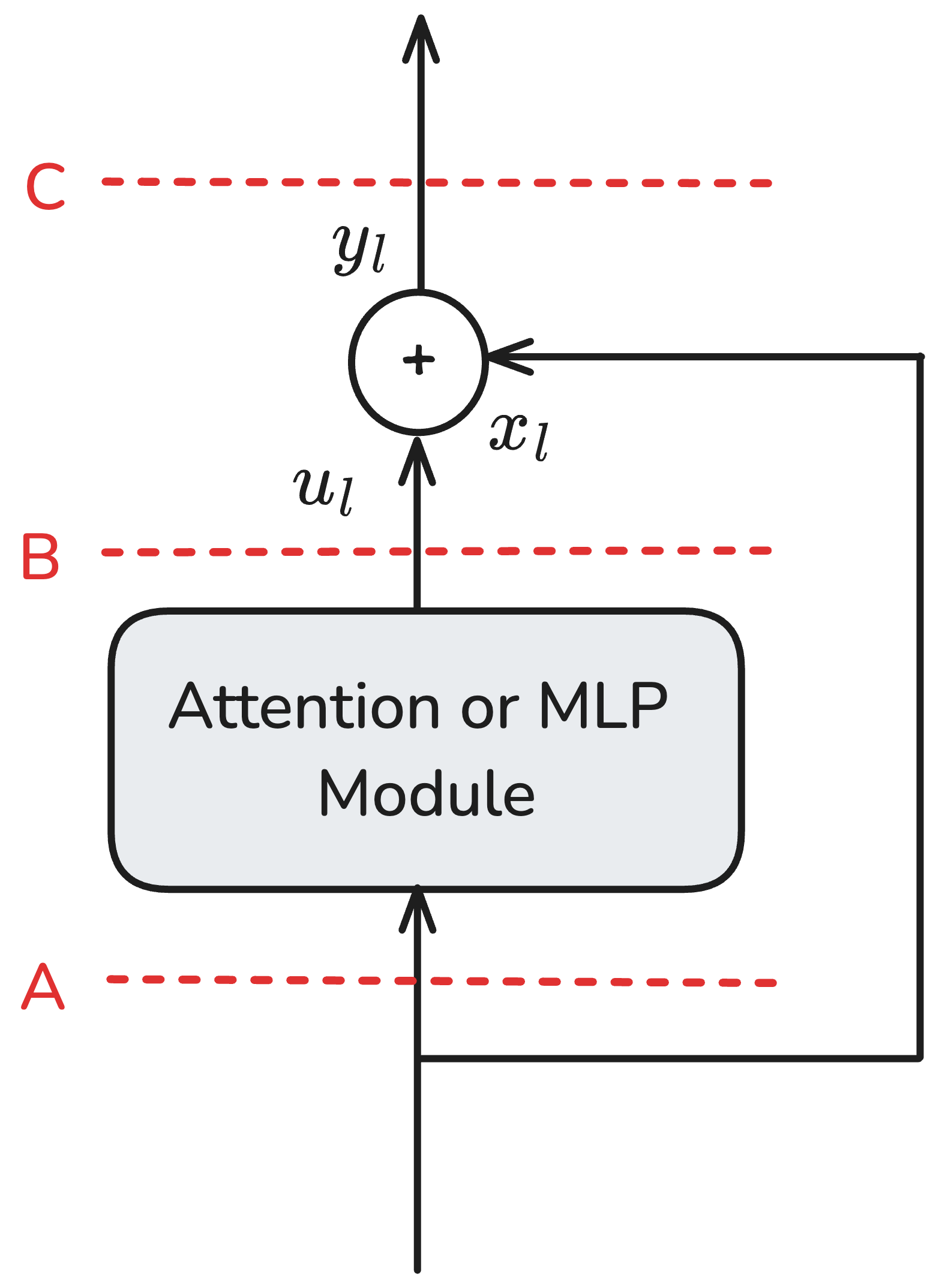
Source: Peri-LN, Figure 2. Position A is the module input, B is the module output before the add, and C is after the residual add. Pre-LN uses A, Peri-LN uses A and B, and Post-LN uses C. The paper’s variance and gradient results are specific to its analysis and models up to 3.2B parameters.

The paper also normalizes input embeddings optionally and the final stack output. Those stack-boundary choices must remain in the manifest; implementing only the per-branch equation is not a complete Peri-LN reproduction.

“Sandwich norm” is a topology family, not one canonical equation

The label is used for several graphs containing both pre- and post-sublayer normalization. A generic branch may be written:

$$y=x+N_o(F(N_i(x))),$$

which overlaps the Peri-LN local equation, while another implementation may normalize the residual sum or insert extra norms inside attention/MLP. Therefore an article, configuration, or checkpoint must provide the ordered graph rather than rely on the nickname. N_i and N_o may have independent affine state; sharing them is another architecture.

Sequential and parallel branches consume different states

Some Transformer variants compute attention and MLP from the same normalized input and add both updates together:

$$y=x+A(N_A(x))+M(N_M(x)).$$

This parallel block is not the sequential Pre-LN block because the MLP no longer reads x + attention_update. Its local Jacobian is:

$$J_{\mathrm{parallel}} =I+J_AJ_{N_A}+J_MJ_{N_M}.$$

For the sequential form:

$$J_{\mathrm{sequential}} =\left(I+J_MJ_{N_M}\right) \left(I+J_AJ_{N_A}\right).$$

Expanding the product reveals the interaction term $J_MJ_{N_M}J_AJ_{N_A}$ that the parallel graph does not contain. The PaLM paper uses a parallel formulation as a systems/architecture choice and reports source-specific training-speed and quality observations. That evidence does not make the two graphs generally equivalent.

Topology registry

Name in this article	One branch equation	Shortcut crosses norm?	Branch output normalized?	Typical stack-final norm
Post-LN	N(x + F(x))	yes	residual sum is normalized	architecture-specific
Pre-LN	x + F(N(x))	no	no	usually yes
Peri-LN	x + N_o(F(N_i(x)))	no	yes	yes in paper contract
parallel Pre-LN	x + A(N_A(x)) + M(N_M(x))	no	no	usually yes
scaled residual	a*x + b*F(N(x)) or paper-specific form	depends	depends	paper-specific

These equations are architecture identities. An optimizer cannot “learn around” loading weights into the wrong graph at inference time.

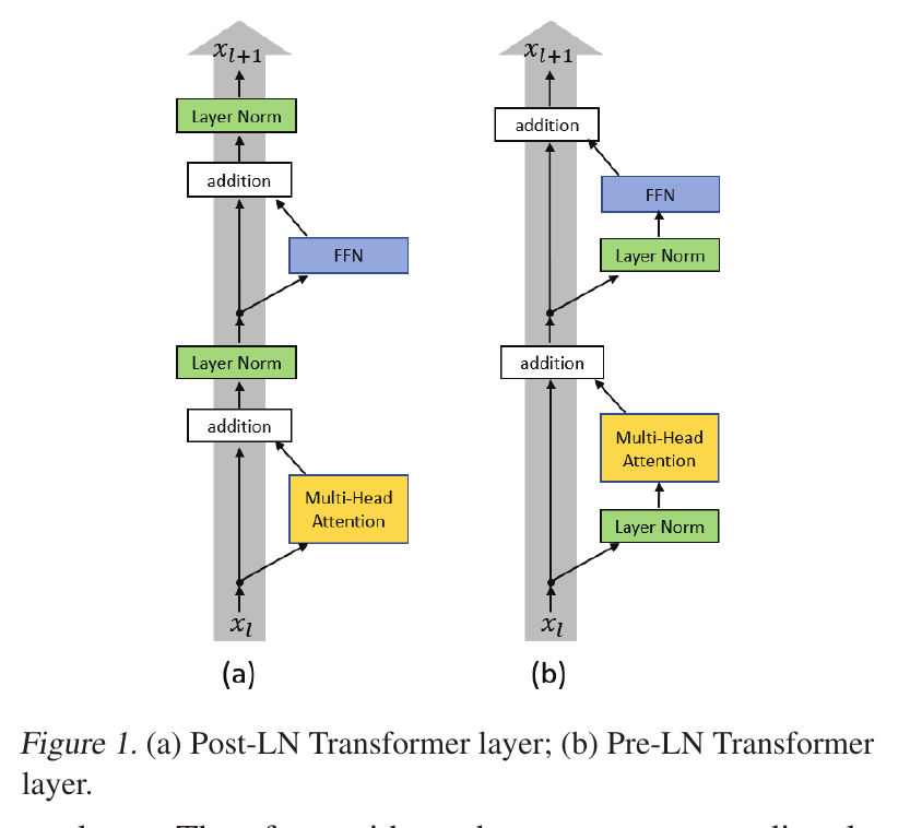
Source: On Layer Normalization in the Transformer Architecture, Figure 1. This replaces the translated derivative used in the source-series article with the paper’s original figure.

Both return [B,S,d_model]. They are nevertheless different computations with different parameter locations and optimization behavior.

Xiong et al. analyze why Post-LN can produce large gradients near the output layers at initialization and why Pre-LN has better-behaved gradients in their setting. This supports treating normalization placement as an optimization-relevant design choice. It does not establish that one ordering is universally superior for every model, training recipe, or target quality level.

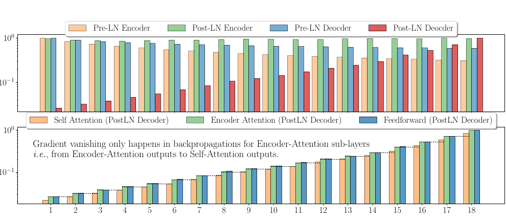
Source: Understanding the Difficulty of Training Transformers, Figure 3. In this 18-layer WMT14 English-German setup, the lower panel isolates gradient decay in Post-LN decoder encoder-attention paths. This is configuration-specific evidence, and the paper explicitly argues that unbalanced gradients alone do not fully explain Transformer training instability.

Backward path: where the identity Jacobian appears

The forward equations also expose a useful local difference in the backward path. Absorb dropout into F for this derivative and treat vectors as column vectors. For Pre-LN:

$$y=x+F(N(x))$$

so the local Jacobian is:

$$J_{\text{pre}} =\frac{\partial y}{\partial x} =I+J_FJ_N$$

and the incoming output gradient becomes:

$$\nabla_x\mathcal{L} =\left(I+J_N^\top J_F^\top\right)\nabla_y\mathcal{L}$$

The I term is a direct contribution from the residual path. That contribution does not pass through the normalization Jacobian for this sublayer.

For Post-LN, first define u = x + F(x) and then y = N(u). The Jacobian is:

$$J_{\text{post}} =J_N(u)\left(I+J_F\right)$$

and:

$$\nabla_x\mathcal{L} =\left(I+J_F^\top\right)J_N(u)^\top\nabla_y\mathcal{L}$$

Here every local route from y back to x first crosses the normalization Jacobian. This algebra explains why the two placements can have different initialization and optimization behavior even though their forward shapes are identical.

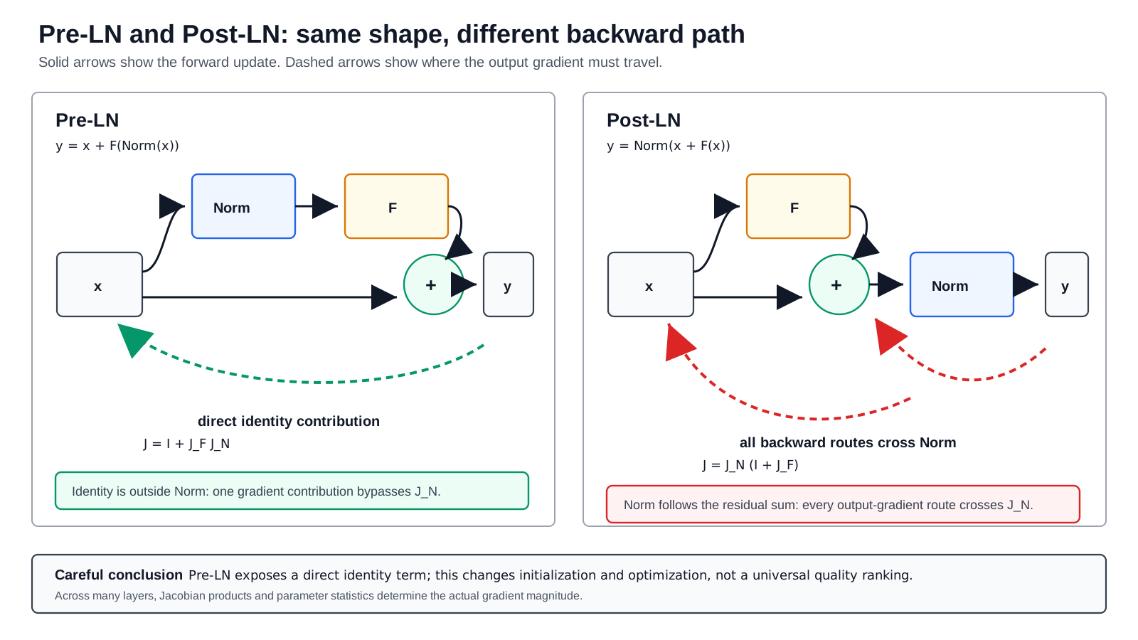
The identity term is not a promise that gradients remain unchanged through an entire deep network. Across layers, the branch Jacobians, normalization statistics, parameter scales, and loss geometry still multiply and interact. The mean-field result from Xiong et al. is correspondingly specific: at initialization in the architectures they analyze, Post-LN has large expected parameter gradients near the output while Pre-LN gradients are better behaved.

Checkpoint rule

same tensors + same norm parameters + different ordering = different model

Do not infer the ordering from shape alone. Read the model class or architecture configuration.

---

0x05 The Harvard SublayerConnection code spine

A14’s central wrapper is:

class SublayerConnection(nn.Module):
    def __init__(self, size, dropout):
        super(SublayerConnection, self).__init__()
        self.norm = LayerNorm(size)
        self.dropout = nn.Dropout(dropout)

    def forward(self, x, sublayer):
        return x + self.dropout(sublayer(self.norm(x)))

Read it inside out:

x:                         [B,S,d_model]
norm(x):                   [B,S,d_model]
sublayer(norm(x)):         [B,S,d_model]
dropout(...):              [B,S,d_model]
x + dropout(...):          [B,S,d_model]

The identity path is the unmodified x. Dropout is applied to the branch result before the addition.

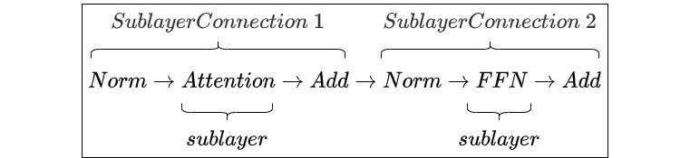
The wrapper accepts a callable sublayer. This keeps attention and MLP implementations separate from the residual/norm policy:

self.sublayer[0](x, lambda x: self.self_attn(x, x, x, mask))
self.sublayer[1](x, self.feed_forward)

Each wrapper clone must own the intended normalization parameters. Reusing one LayerNorm instance for unrelated branches changes the parameter-sharing contract.

---

0x06 Encoder block assembly

The Harvard encoder layer composes two Pre-LN residual updates:

class EncoderLayer(nn.Module):
    def forward(self, x, mask):
        x = self.sublayer[0](
            x,
            lambda x: self.self_attn(x, x, x, mask),
        )
        return self.sublayer[1](x, self.feed_forward)

Expanded without the wrapper abstraction:

attn_update = self.self_attn(
    self.norm_1(x),
    self.norm_1(x),
    self.norm_1(x),
    mask,
)
x = x + self.dropout_1(attn_update)

ffn_update = self.feed_forward(self.norm_2(x))
x = x + self.dropout_2(ffn_update)

The expanded form is conceptual. An implementation should avoid computing the same normalization three times; it would normally bind x_norm = norm_1(x) once before creating Q, K, and V.

Shape path:

encoder x:              [B,S,d_model]
self-attention update:  [B,S,d_model]
after residual 1:       [B,S,d_model]
MLP update:             [B,S,d_model]
after residual 2:       [B,S,d_model]

The attention branch mixes rows. The MLP branch transforms channels per row. The wrappers preserve and update the residual state.

---

0x07 Encoder-decoder block assembly

An encoder-decoder Transformer decoder has three residual branches:

class DecoderLayer(nn.Module):
    def forward(self, x, memory, src_mask, tgt_mask):
        m = memory
        x = self.sublayer[0](
            x,
            lambda x: self.self_attn(x, x, x, tgt_mask),
        )
        x = self.sublayer[1](
            x,
            lambda x: self.src_attn(x, m, m, src_mask),
        )
        return self.sublayer[2](x, self.feed_forward)

The state ownership is:

decoder x:             [B,T,d_model]
encoder memory m:      [B,S,d_model]

masked self-attn:
    query rows from x
    output [B,T,d_model]
    residual adds to x

cross-attn:
    query rows from x
    key/value rows from m
    output [B,T,d_model]
    residual adds to decoder x

MLP:
    transforms each decoder row
    output [B,T,d_model]
    residual adds to decoder x

Cross-attention does not add encoder memory directly to decoder state. Its output is target-indexed because query length determines output length. M3.2 owns the full Q/K/V source and mask semantics; M3.7 owns the three residual wrappers.

---

0x08 Modern decoder-only assembly: LLaMA-style Pre-RMSNorm

A modern decoder-only block typically has no encoder memory and no cross-attention branch. The verified Transformers v5.13.1 LLaMA layer uses RMSNorm before both self-attention and the MLP:

residual = hidden_states
hidden_states = self.input_layernorm(hidden_states)
hidden_states, _ = self.self_attn(
    hidden_states=hidden_states,
    attention_mask=attention_mask,
    position_embeddings=position_embeddings,
    past_key_values=past_key_values,
    **kwargs,
)
hidden_states = residual + hidden_states

residual = hidden_states
hidden_states = self.post_attention_layernorm(hidden_states)
hidden_states = self.mlp(hidden_states)
hidden_states = residual + hidden_states

Block equation:

$$h= x+\operatorname{Attn}(\operatorname{RMSNorm}_1(x))$$ $$y= h+\operatorname{MLP}(\operatorname{RMSNorm}_2(h))$$

The member name post_attention_layernorm can be misleading. It is located after the attention residual update in block order, but it is a pre-norm for the MLP branch. It does not make the block Post-LN.

The code also does not add residual-branch dropout. That is an architectural choice, not an omission to repair by copying the Harvard wrapper. Attention-probability dropout may still be configured inside the attention implementation.

Shape path:

hidden_states:                 [B,S,d_model]
input_layernorm(...):          [B,S,d_model]
self_attn(...):                [B,S,d_model]
first residual add:            [B,S,d_model]
post_attention_layernorm(...): [B,S,d_model]
mlp(...):                      [B,S,d_model]
second residual add:           [B,S,d_model]

---

0x09 Why a Pre-LN stack usually has a final norm

In Post-LN, each sublayer update ends with normalization. In Pre-LN, the residual state leaves the final branch without a normalization applied after the add:

y = x + F(norm(x))

The Harvard encoder and decoder therefore apply a final normalization after all layers:

class Encoder(nn.Module):
    def forward(self, x, mask):
        for layer in self.layers:
            x = layer(x, mask)
        return self.norm(x)

The same Transformers v5.13.1 LLaMA implementation applies a final RMSNorm after the decoder layers:

for decoder_layer in self.layers:
    hidden_states = decoder_layer(hidden_states, ...)

hidden_states = self.norm(hidden_states)

That final norm is part of the model function:

last block state: [B,S,d_model]
final norm:       [B,S,d_model]
output head:      [B,S,vocab_size] or [B,vocab_size]

Omitting it preserves shape while changing every downstream logit. M3.8 begins from the final normalized hidden state expected by the checkpoint, not merely the raw output of the last residual addition.

---

0x09A Depth scaling and normalization variants

Pre-LN and Post-LN are reference points, not the end of the design space. Later methods change at least one of four contracts:

where normalization sits;
which statistic it computes;
how the residual and branch are scaled;
whether normalization is replaced by a bounded nonlinear transform.

Residual scaling and initialization

For

$$x_{l+1}=x_l+\alpha_lF_l(x_l),$$

$\alpha_l$ controls the initial update magnitude and its gradient. Common engineering patterns include fixed depth scaling, learned residual gates initialized near zero, zero-initialized branch-output projections, and architecture-specific gains for input and output projections.

These are not interchangeable if the checkpoint was trained under one specific rule. A scaling factor can be folded into a weight tensor for inference only if doing so preserves dtype, quantization, and weight-sharing semantics.

The useful comparison unit is therefore not a method name but a recipe contract:

(ordered graph,
 branch count and depth convention,
 parameter initialization,
 new learned state,
 optimizer / warmup / regularization assumptions,
 training-time profiling,
 inference-time reparameterization)

Changing only the coefficient in the residual equation does not reproduce a paper whose result depends on all seven fields.

Why inverse powers of depth appear

Suppose a stack has $L$ residual branches whose initial outputs are centered, independent for this toy derivation, and each has coordinate variance $\sigma_F^2$:

$$x_L=x_0+\sum_{l=0}^{L-1}a_lF_l(x_l).$$

Ignoring branch-state correlation gives the accounting approximation

$$\operatorname{Var}(x_L-x_0) \approx \sigma_F^2\sum_{l=0}^{L-1}a_l^2.$$

With one shared scale $a$, an $O(1)$ accumulated update requires $La^2=O(1)$, hence $a=O(L^{-1/2})$. This explains the recurring branch scale, but not yet a weight-initialization exponent. If a branch contains $m$ weight layers and each weight is scaled by $s$, its leading output scale is $s^m$. Matching $s^m=O(L^{-1/2})$ gives

$$s=O\!\left(L^{-1/(2m)}\right).$$

This is a forward-variance baseline, not the final Fixup exponent. The derivation is intentionally limited: attention softmax, correlated branches, normalization, dropout, adaptive-optimizer state, and encoder-decoder coupling break the independent linear-branch model. T-Fixup, Admin, DeepNorm, and DeepScaleLM introduce different analyses precisely because a Transformer is not this toy stack.

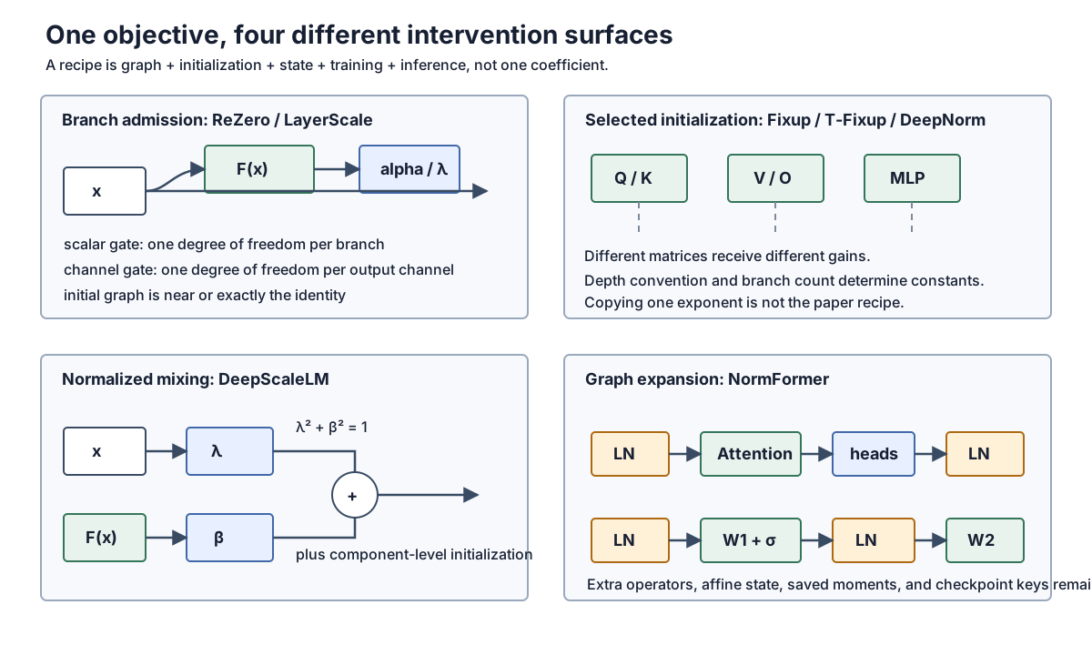
ReZero and LayerScale: learned branch admission

ReZero writes a residual branch as

$$x_{l+1}=x_l+\alpha_lF_l(x_l),\qquad \alpha_l=0\text{ at initialization}.$$

At initialization, the branch output and its parameter gradients are gated by zero, while the state Jacobian is exactly the identity:

$$\left.\frac{\partial x_{l+1}}{\partial x_l}\right|_{\alpha_l=0}=I.$$

The gate itself can receive a gradient $\partial\mathcal L/\partial\alpha_l=\langle\nabla_{x_{l+1}}\mathcal L, F_l(x_l)\rangle$, allowing the branch to enter training. ReZero’s paper removes normalization in its studied architecture; attaching a zero gate while retaining an arbitrary Pre-LN graph is a related engineering variant, not the same paper contract.

LayerScale replaces the one scalar with one learned diagonal gain per branch output:

$$h=x+\operatorname{diag}(\lambda_A)A(N(x)),$$ $$y=h+\operatorname{diag}(\lambda_M)M(N(h)).$$

The cited CaiT recipe keeps Pre-LN and warmup, initializes every channel gain to a small $\epsilon$, and varies $\epsilon$ with the tested vision-transformer depth. It therefore differs from ReZero in gate granularity, nonzero initialization, retained normalization, warmup, task, and training recipe. Its diagonal gains may be folded into compatible output projections for inference, but they remain checkpoint state during training and before such a verified fold.

Fixup and T-Fixup: initialization is the method

Fixup is a residual-network recipe, not a generic instruction to divide Transformer weights by depth. For an $L$-branch network with $m$ weight layers per residual branch, its contract includes:

zero-initialize the last weight layer in every residual branch and the classifier;
scale the other branch weights by L^(-1/(2m-2));
add a branch scalar initialized to 1;
add scalar biases before weight layers and nonlinearities;
remove normalization in the studied residual network.

The exponent differs from the toy $L^{-1/(2m)}$ result because Fixup analyzes the magnitude of a full parameter update, including derivatives with respect to each branch weight, rather than only the forward branch output.

T-Fixup derives a separate encoder-decoder Transformer contract. For $N$ encoder and $N$ decoder layers in the paper’s convention:

1. Xavier-initialize non-embedding parameters.
2. Initialize input embeddings from N(0, d^(-1/2)).
3. Scale decoder V/O attention matrices, decoder MLP weights,
   and encoder/decoder input embeddings by (9N)^(-1/4).
4. Scale encoder V/O attention matrices and encoder MLP weights
   by 0.67 * N^(-1/4).
5. Remove every LayerNorm and train without learning-rate warmup.

Q and K are not in the selected scaled set. The constants follow the paper’s encoder-decoder block count and update-magnitude analysis; applying them unchanged to a decoder-only LLaMA block is not T-Fixup. The paper’s source-reported training result is evidence for its NMT configurations, not a universal recommendation to remove modern decoder RMSNorm.

Admin: data-dependent initialization and a foldable shortcut vector

Admin starts from the paper’s residual-dependency and perturbation-amplification analysis. It changes a Post-LN sublayer to

$$x_i=\operatorname{LN}(b_i),\qquad b_i=\omega_i\odot x_{i-1}+F_i(x_{i-1}).$$

This is not ordinary learned residual scaling. Admin first performs a profiling forward pass with $\omega_i=1$, records each earlier branch-output variance, and then initializes

$$\omega_i =\sqrt{\sum_{j<i}\operatorname{Var}(F_j(x_{j-1}))}.$$

The profile batch, model mode, dropout policy, dtype, and distributed reduction are therefore initialization inputs. The paper uses no more than 8,192 tokens for this profiling step in its experiments and supplies an exact reparameterization that can absorb $\omega_i$ into compatible LayerNorm and branch weights after training. That fold has module-specific formulas; deleting the vector without applying them changes the function.

DeepNorm

DeepNorm modifies the residual equation and parameter initialization to train very deep Post-LN Transformers:

$$x_{l+1} =\operatorname{LayerNorm} \left(\alpha x_l+G_l(x_l;\theta_l)\right),$$

while selected branch weights use an initialization gain $\beta$. For a decoder-only stack of $M$ layers, the paper gives one contract:

$$\alpha=(2M)^{1/4}, \qquad \beta=(8M)^{-1/4}.$$

Encoder-only and encoder-decoder architectures use different formulas because their branch counts and interactions differ. Copying the decoder-only constants into an encoder-decoder is not DeepNorm.

The complete architecture table from the paper is:

Architecture	Encoder $(\alpha_e,\beta_e)$	Decoder $(\alpha_d,\beta_d)$
encoder-only, $N$ layers	$((2N)^{1/4},(8N)^{-1/4})$	not present
decoder-only, $M$ layers	not present	$((2M)^{1/4},(8M)^{-1/4})$
encoder-decoder	$(0.81(N^4M)^{1/16},\;0.87(N^4M)^{-1/16})$	$((3M)^{1/4},(12M)^{-1/4})$

The initialization first applies a standard method such as Xavier and then scales FFN weights plus attention value and output projections by $\beta$. Query and key projections keep gain one. The shortcut inside every Post-LN sublayer uses its architecture-side $\alpha$. The paper derives these constants by bounding the expected model-update magnitude under an SGD analysis and then tests the recipe with Adam; the theorem is not an optimizer-independent proof of convergence.

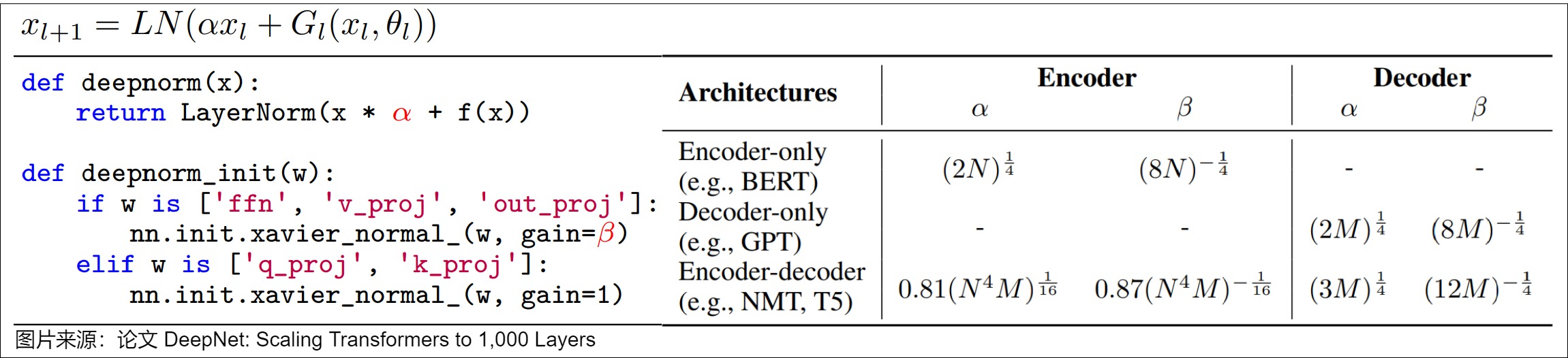
DeepNorm is a training recipe and architecture contract. At inference, $\alpha$ remains part of the residual computation unless it has been exactly folded into compatible parameters.

DeepScaleLM: normalize the add, then initialize every component

DeepScaleLM uses two fixed coefficients:

$$x_{l+1}=\lambda x_l+\beta F_l(x_l), \qquad \lambda^2+\beta^2=1.$$

If skip and branch each have unit variance and zero covariance, this identity gives unit output variance directly. The simplified paper recipe chooses

$$\beta^2=\frac{2}{N}, \qquad \lambda^2=1-\frac{2}{N},$$

then separately initializes embeddings, Q/K, V/output, and FFN weights from component-level moment equations. The full method tracks token correlation, dropout, nonlinear means, and layer-dependent attention output scales; the two coefficients alone are not DeepScaleLM. The paper also describes a verified inference fold into normalization gains and output projections. This is a 2024 paper with source-reported results across its chosen language, speech, and vision setups; it should be reproduced from its code/formulas rather than treated as a settled default.

ScaleNorm

ScaleNorm replaces per-channel affine normalization with a learned scalar scale:

$$\operatorname{ScaleNorm}(x) =g\frac{x}{\|x\|_2}.$$

Compared with RMSNorm,

$$\operatorname{RMS}(x)=\frac{\|x\|_2}{\sqrt d},$$

so a scale-only RMSNorm with a shared scalar is equivalent up to the $\sqrt d$ factor. Standard RMSNorm learns one scale per channel and therefore has more affine freedom.

Sandwich and additional normalization

Some architectures add norms before and after selected sublayers or inside attention/MLP computations. NormFormer, for example, keeps the Pre-LN input norms and changes both branches:

$$\operatorname{NormScaledMHA}(x) =x+\operatorname{LN}(\operatorname{HeadScaleMHA}(\operatorname{LN}(x))),$$ $$\operatorname{NormFFN}(x) =x+\operatorname{LN}(\sigma(\operatorname{LN}(x)W_1+b_1))W_2+b_2.$$

Its complete recipe adds a post-attention LayerNorm, per-head attention-output scales, and a LayerNorm after the first FFN projection and activation. The paper also studies a separate per-channel residual-scaling option initialized to one, but does not use it for the reported 1.3B and 2.7B causal models because it hurt performance there. “NormFormer” therefore cannot be reconstructed by inserting one extra norm after an arbitrary block.

These are not cosmetic stability helpers: every added norm owns parameters, reductions, epsilon, placement, saved backward state, and a state-dict entry.

QK-Norm is a separate example: it normalizes query/key head vectors before their dot product. It changes attention-score geometry and belongs to M3.1/M3.2, even if a configuration calls it a normalization variant. It must not be confused with normalizing the residual stream.

Training and inference contract comparison

Method	Normalization graph	New state	Data-dependent init	Training assumptions in source	Inference consequence
ReZero	removed in paper setup	scalar gate per residual branch	no	gate starts at zero	gate remains or is folded
LayerScale	retained Pre-LN	channel gain per branch	no	warmup and vision recipe retained	diagonal gain remains or folds into output weight
Fixup	removed	branch scalar + scalar biases	no	full initialization and regularization recipe	added scalar state remains/folds
T-Fixup	removed	no norm affine state	no	no warmup; paper-specific NMT initialization	ordinary linear graph with trained scaled weights
Admin	Post-LN	shortcut vector $\omega_i$	yes, profile pass	standard initialization plus profile/reinitialize	paper gives module-specific exact fold
DeepNorm	scaled Post-LN	ordinary norm state + fixed $\alpha$	no	architecture-specific $\alpha/\beta$ and selected matrices	scaled shortcut remains unless folded
DeepScaleLM	scaled add with Pre- or Post-LN analysis	fixed $\lambda,\beta$ plus ordinary model state	analytic correlation model, not a profile pass	component moment initialization + residual scaling	paper gives a weight/norm fold
NormFormer	expanded Pre-LN graph	extra norms + head scales	no	paper-specific LR tuning and compute matching	extra operators and checkpoint keys remain

The table compares contracts, not benchmark rank. A method can be mathematically foldable yet still expensive to migrate into an existing checkpoint because optimizer state, quantization scales, tied weights, and fused-kernel support may not obey the same reparameterization.

Alternatives must be compared as state machines

The following papers are often grouped under “better normalization,” but they change four different ownership surfaces. RealFormer adds a transient tensor to the attention interface. nGPT constrains hidden states and parameters to hyperspheres. Dynamic Tanh replaces a moment-reduction operator with a learned elementwise nonlinearity. PRepBN changes both the training schedule and the inference state. Shape compatibility is therefore not a migration argument.

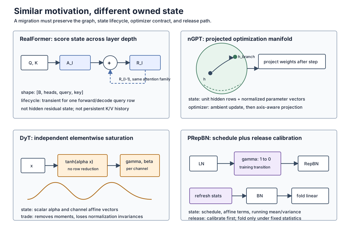
RealFormer: a residual stream over attention scores

RealFormer retains the ordinary Transformer hidden-state residual and adds a second route over raw pre-softmax attention scores. For one attention family, let the current layer produce

$$A_l=\frac{Q_lK_l^\top}{\sqrt{d_h}} \in\mathbb{R}^{B\times h\times S_q\times S_k}.$$

With $R_0=0$, the running-sum variant is

$$R_l=A_l+R_{l-1}, \qquad P_l=\operatorname{softmax}(R_l+M,\,-1),$$

where the additive visibility mask $M$ still belongs immediately before the softmax. The paper’s running-mean alternative divides out the number of scores that have entered the route:

$$\bar R_l =\frac{(l-1)\bar R_{l-1}+A_l}{l}.$$

This is not a cosmetic rewrite. The running sum can grow approximately linearly with traversed depth when score statistics align; the running mean changes that scale and can be interpreted as a depth-dependent softmax temperature. The paper used running sum by default in its BERT and ETC experiments and reported running mean as useful in some deeper translation settings. Those are source-reported recipe choices, not a universal ordering.

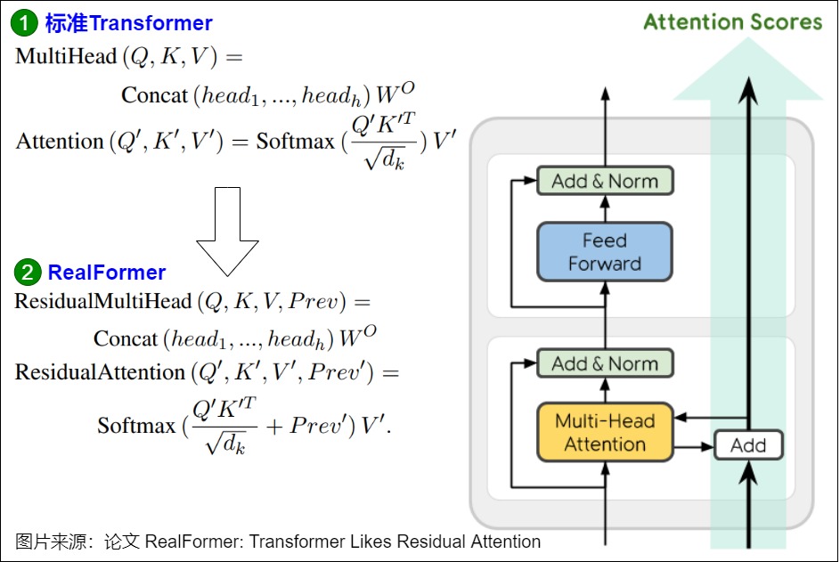
The executable interface must return both the value mixture and the new score state:

def realformer_attention(q, k, v, additive_mask, previous_scores=None, depth=None):
    local_scores = q @ k.transpose(-2, -1) / sqrt(q.shape[-1])

    if previous_scores is None:
        residual_scores = local_scores
    elif depth is None:  # running sum
        residual_scores = previous_scores + local_scores
    else:                # previous_scores stores the running mean
        residual_scores = ((depth - 1) * previous_scores + local_scores) / depth

    probabilities = softmax(residual_scores + additive_mask, dim=-1)
    output = probabilities @ v
    return output, residual_scores

The score state has shape [B, heads, query_length, key_length]; the hidden residual remains [B, sequence, d_model]. In autoregressive decode, only the current query row needs to travel through layer depth for the current target step. It is not a second history cache analogous to K/V. If a model has encoder self-attention, decoder self-attention, and cross-attention, each attention family needs an independent score route because their query/key axes and masks differ. A state-dict can remain parameter-compatible while the runtime ABI is not.

nGPT: the whole optimization manifold changes

nGPT does not merely replace RMSNorm. It interprets each hidden row as a point on the unit hypersphere and each attention/MLP branch as a proposed destination. Starting from linear interpolation,

$$\operatorname{LERP}(a,b;\alpha) =(1-\alpha)a+\alpha b =a+\alpha(b-a),$$

the paper generalizes the scalar step to non-negative per-channel eigen learning rates. For the two updates in layer $l$,

$$h_A=\operatorname{Norm}(\operatorname{ATTN}(h)), \qquad h\leftarrow\operatorname{Norm} \left(h+\alpha_A\odot(h_A-h)\right),$$ $$h_M=\operatorname{Norm}(\operatorname{MLP}(h)), \qquad h\leftarrow\operatorname{Norm} \left(h+\alpha_M\odot(h_M-h)\right).$$

The outer Norm is a projection/retraction back to unit length, not a learned RMSNorm layer. When every coordinate of $\alpha$ lies in $[0,1]$, the pre-projection point is a coordinate-wise interpolation; learned vector rates also define a diagonal variable metric. This is already a different residual algebra from h + branch(h).

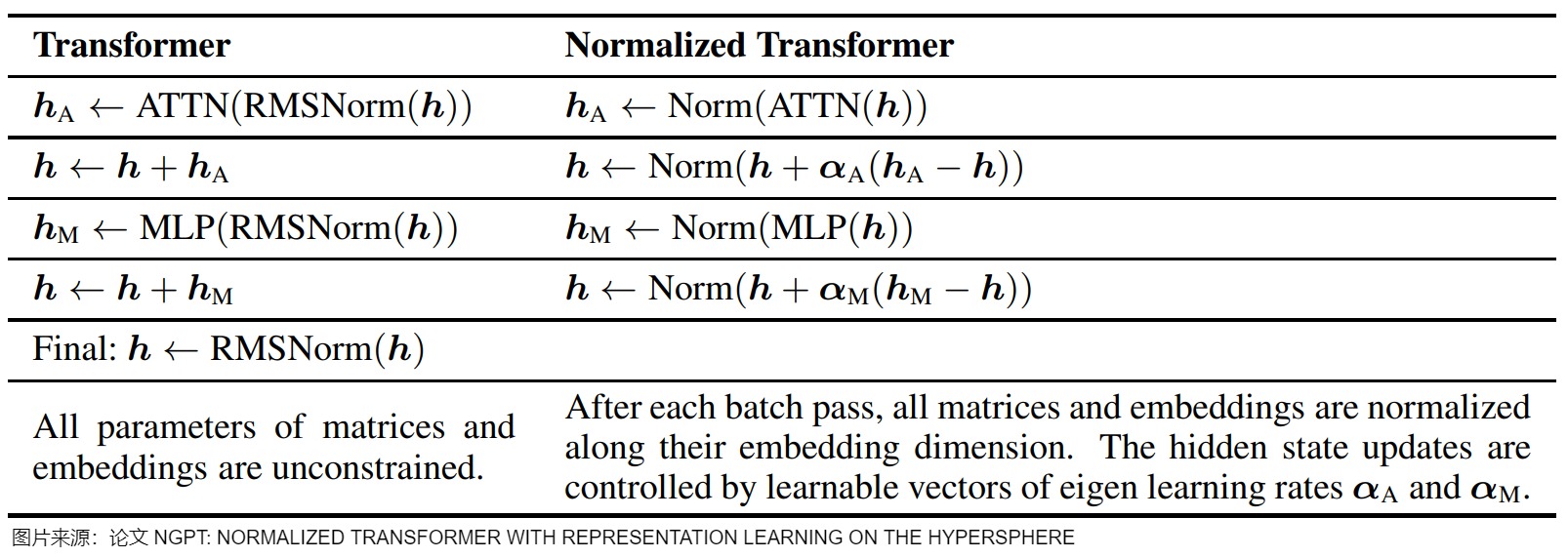
The full paper contract is broader still:

1. Remove LayerNorm/RMSNorm operators, including the final norm.
2. Constrain input/output embeddings and $W_q,W_k,W_v,W_o,W_u,W_\nu,W_o^{MLP}$ along their embedding-vector axes after each optimizer step; optional forward normalization can defend the invariant as well.
3. Use the two normalized interpolation updates above. The paper initializes $\alpha_A$ and $\alpha_M$ at 0.05 and uses a separate parameter scaling to control their effective Adam learning rate.
4. Normalize projected $q$ and $k$, apply a learned vector $s_{qk}$, and replace the baseline $1/\sqrt{d_h}$ score factor with $\sqrt{d_h}$. Unit-normalized dot products have variance on the order of $1/d_h$, which motivates the reversed scale.
5. Normalize the MLP matrices and restore useful magnitudes with learned $s_u,s_\nu$; the paper multiplies the nonlinear gate input by $\sqrt{d_{model}}$.
6. Add a learned vocabulary-logit scale because normalized embeddings bound cosine logits.
7. Remove weight decay and learning-rate warmup in the reported nGPT recipe.

def ngpt_block(h, alpha_attn, alpha_mlp):
    h_attn = unit_norm(attention(h), dim=-1)
    h = unit_norm(h + positive(alpha_attn) * (h_attn - h), dim=-1)

    h_mlp = unit_norm(mlp(h), dim=-1)
    h = unit_norm(h + positive(alpha_mlp) * (h_mlp - h), dim=-1)
    return h

@no_grad()
def project_ngpt_parameters(model):
    for parameter, embedding_axis in model.hyperspherical_parameters():
        parameter.copy_(unit_norm(parameter, dim=embedding_axis))

The axis metadata in hyperspherical_parameters() is part of the model manifest: blindly normalizing every matrix along dim=-1 can constrain the wrong vectors. Optimizer moments are updated in ambient coordinates while the parameters are projected afterward, so exact resume also requires the same projection schedule and parameter-scaling metadata. An RMSNorm checkpoint cannot be converted into nGPT by deleting norm modules after training.

Dynamic Tanh: an elementwise saturating transform, not normalization

Dynamic Tanh proposes

$$\operatorname{DyT}(x) =\gamma\odot\tanh(\alpha x)+\beta,$$

where $\alpha$ is one learned scalar and $\gamma,\beta\in\mathbb{R}^d$ are learned channel vectors. The derivative makes the changed geometry explicit:

$$\frac{\partial\operatorname{DyT}(x_i)}{\partial x_i} =\gamma_i\alpha\left(1-\tanh^2(\alpha x_i)\right).$$

Near zero the map is approximately affine with slope $\gamma_i\alpha$; in the tails the output saturates and the derivative approaches zero. Unlike LayerNorm/RMSNorm, one row does not depend on any other coordinate of that row. There is no moment reduction, no shift/scale invariance guarantee, and no normalization statistic to save for backward.

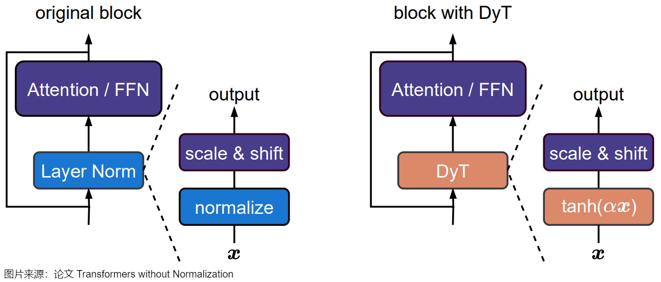
The paper motivates DyT with aggregate input/output plots from trained normalization layers. Those plots show tanh-like envelopes in selected deeper layers; they do not mean LayerNorm is an elementwise tanh. For one fixed row, LayerNorm’s mean and variance are shared across coordinates, so its mapping is affine once those row statistics are fixed. The S-shape emerges from pooling many rows with different statistics.

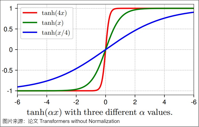
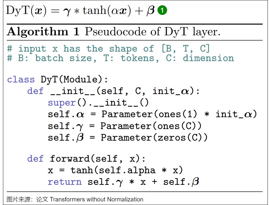
class DynamicTanh(Module):
    def __init__(self, width, alpha_init=0.5):
        self.alpha = Parameter(full((), alpha_init))
        self.gamma = Parameter(ones(width))
        self.beta = Parameter(zeros(width))

    def forward(self, x):
        return self.gamma * tanh(self.alpha * x) + self.beta

The paper initializes $\gamma=1$ and $\beta=0$. It uses $\alpha_0=0.5$ as the default for non-LLM models, but reports that LLM width and norm location require separate tuning. Its source-reported attention/other initializations are 0.8/0.2, 0.6/0.15, and 0.2/0.05 for the evaluated 7B, 13B, and 34B/70B LLaMA configurations. Those values are evidence from that recipe, not a scaling law. The LLaMA experiments also add a learned post-embedding scalar initialized to $\sqrt{d_{model}}$ because the initial activation magnitude was otherwise too small. It replaces every RMSNorm site, including the final norm, and retrains under that graph. Therefore “drop-in” describes the experiment’s module-level substitution, not checkpoint-equivalent post-training replacement. The paper’s uncompiled H100 microbenchmarks and compiled results also differ: removing a reduction creates an optimization opportunity, not a hardware-independent latency guarantee.

PRepBN: progressive graph migration plus offline statistics

PRepBN addresses a different problem: retain LayerNorm’s training path early, then end with a BatchNorm-family graph whose running statistics can be used at inference. Its RepBN branch is

$$\operatorname{RepBN}(X)=\operatorname{BN}(X)+\eta X.$$

If BatchNorm is written

$$\operatorname{BN}(X;\mu,\sigma,a,b) =a\frac{X-\mu}{\sigma}+b,$$

then the identity term can be folded exactly:

$$\operatorname{RepBN}(X;\mu,\sigma,a,b) =\operatorname{BN}(X;\mu,\sigma,a+\eta\sigma,b+\eta\mu).$$

Expanding the right side gives $a(X-\mu)/\sigma+b+\eta(X-\mu)+\eta\mu =\operatorname{BN}(X)+\eta X$, which proves the reparameterization for fixed statistics. It does not remove the need to estimate and freeze valid $\mu,\sigma$.

During training, the paper mixes LayerNorm and RepBN:

$$\operatorname{PRepBN}_t(X) =\gamma_t\operatorname{LN}(X) +(1-\gamma_t)\operatorname{RepBN}(X), \qquad \gamma_t=\operatorname{clip}\left(\frac{T-t}{T},0,1\right).$$

At $t=0$, LayerNorm owns the output; at $t=T$, the graph is pure RepBN. The paper also discusses cosine and step schedules but uses a linear transition as its simple default. After training, RepBN is converted to BN and then can be folded into an adjacent linear operator under fixed inference statistics.

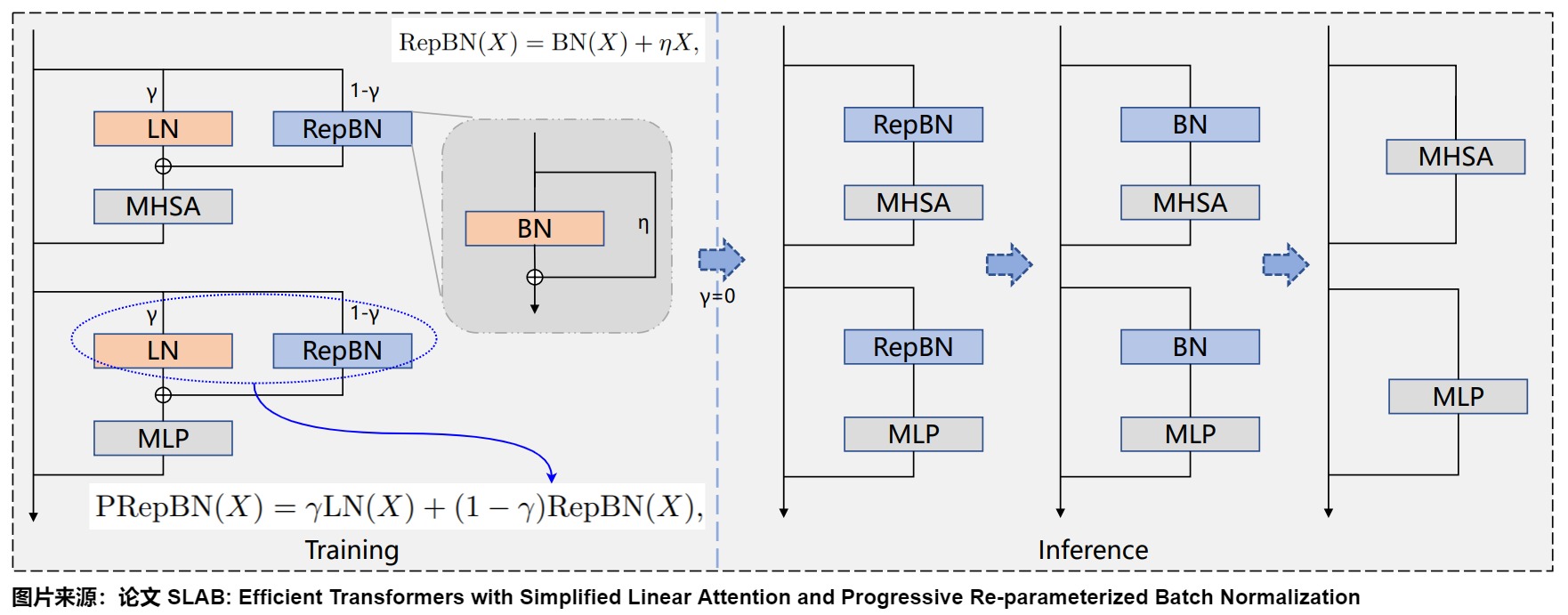
def prepbn(x, step, transition_steps, layer_norm, rep_batch_norm):
    gamma = clamp((transition_steps - step) / transition_steps, 0.0, 1.0)
    return gamma * layer_norm(x) + (1.0 - gamma) * rep_batch_norm(x)

# Release preparation after the transition is complete:
freeze_model_parameters()
refresh_batchnorm_running_statistics(calibration_loader)
fold_repbn_identity_into_batchnorm()
fold_batchnorm_into_adjacent_linear_where_legal()

The calibration lifecycle is not optional bookkeeping. In the paper’s vision-transformer recipe, DropPath shifted activation variance, so the authors froze model parameters and updated RepBN statistics for ten additional epochs. Batch composition, padding policy, distributed statistic aggregation, and train/eval mode now affect the released function. The evidence is primarily vision-centric; this article does not promote PRepBN to a universal decoder-only LLM replacement.

Paper-by-contract comparison

Method	What changes	New state and lifecycle	Training contract	Runtime consequence	Invalid shortcut
LayerNorm	row-standardization operator	learned $\gamma,\beta$; per-row moments	ordinary end-to-end training	row reductions at every call	use batch statistics
RMSNorm	row RMS operator	learned scale; per-row mean square	ordinary end-to-end training	one square-reduction family	assume centering
RealFormer	attention interface	transient score route per attention family	train graph with running sum or mean	extra score add/storage; no new parameters	treat score route as hidden residual or KV cache
nGPT	hidden update, parameter manifold, attention/MLP/logit scales	projected matrices/embeddings and vector update rates	full nGPT optimizer/projection recipe	repeated vector normalization and no final norm	delete RMSNorm from a trained checkpoint
DyT	normalization sites	scalar $\alpha$, channel $\gamma,\beta$	retrain substituted graph; LLM embedding scale in paper	elementwise tanh, no moment reduction	claim scale invariance or checkpoint equivalence
PRepBN	norm graph across training time	schedule, BN affine state, running statistics, calibration	progressive LN-to-RepBN transition	fixed-stat BN/linear folds at release	skip statistic refresh or deploy with $\gamma_t>0$

Source-reported speed, convergence, depth, or quality improvements belong to each paper’s architecture, optimizer, data, hardware, and evaluation setup. The comparison above is about reconstructing functions and state lifecycles, not a universal benchmark ranking.

---

0x0A Dropout has multiple owners

“Transformer dropout” is not one tensor or one location.

Dropout object	Typical location	Local owner
attention-probability dropout	after softmax, before P_attn @ V	M3.1
MLP hidden dropout	after activation in the classic Harvard FFN	M3.6
residual-branch dropout	after attention/MLP output, before residual add	M3.7
embedding/position dropout	before the block stack in some architectures	M2 / model input boundary

Harvard Pre-LN branch:

y = x + dropout(sublayer(norm(x)))

Original Post-LN branch:

y = norm(x + dropout(sublayer(x)))

In both cases the branch result is dropped before the residual addition. Dropping the identity path instead changes the state-preservation mechanism.

Dropout is active during training and disabled in evaluation mode under normal nn.Dropout use. A model can expose separate probabilities for attention weights, hidden activations, and residual branches. One field should not be assumed to control all three.

Stochastic depth is not elementwise dropout

Stochastic depth / DropPath samples whether an entire branch update participates, often per example:

$$y=x+\frac{z}{1-p}F(x), \qquad z\sim\operatorname{Bernoulli}(1-p).$$

Elementwise dropout samples many coordinates inside F(x); DropPath scales or removes the whole branch for a sample. Their expected branch output can match under inverted scaling, but their covariance and training dynamics differ. A checkpoint trained with one should not silently execute the other.

Inverted branch dropout preserves a mean, not a realization

For one branch element $u_j$ and keep probability $q=1-p$:

$$\tilde u_j=\frac{m_j}{q}u_j, \qquad m_j\sim\operatorname{Bernoulli}(q).$$

Conditioned on the deterministic branch value:

$$\mathbb E[\tilde u_j\mid u_j]=u_j,$$ $$\operatorname{Var}(\tilde u_j\mid u_j) =\frac{p}{1-p}u_j^2.$$

Thus training-time x + dropout(u) is an unbiased estimator of x + u per element, but its realized norm, covariance, and downstream normalization statistics differ. The statement also assumes the mask is sampled independently of u under the declared RNG policy.

Mask granularity is architecture state:

Policy	Typical mask broadcast	What one draw removes
elementwise branch dropout	[B,S,D]	individual update coordinates
channel dropout	[B,1,D] or method-specific	update channels across rows
token/row dropout	[B,S,1]	complete token-row updates
stochastic depth / DropPath	[B,1,1]	a complete branch for one example
global layer skip	scalar or synchronized policy	a layer for the whole step/model path

The last policy overlaps depth pruning/training methods such as LayerDrop and is owned in full by M6. M3.7 owns only the local stochastic wrapper and its state.

RNG identity belongs to backward and recomputation

Autograd may save a concrete mask. Activation checkpointing may instead save a seed/counter and regenerate the mask. Correct replay requires the regenerated decision to be a function of stable logical coordinates, for example:

(global_step, microbatch_id, layer_id, branch_id, token_row, channel)

Kernel launch order, tensor-parallel rank, or tile scheduling should not silently change the logical random field. A new mask during recomputation gives a forward value from one graph and gradients from another.

The dropout paper supplies the general stochastic-regularization lineage; the exact Transformer placement, broadcast shape, inverted scaling, and replay mechanism come from the model and runtime contract.

---

0x0AA Local state, reduction, and residual-update ledger

Normalization preserves shape, but it is not cost-free. For:

x: [B,S,d_model]

the residual stream contains:

$$N_x=BSd_{model}$$

elements. One residual merge performs B*S*d_model elementwise additions. A decoder-only block with attention and MLP branches performs two such merges. An original encoder layer also has two, while an encoder-decoder decoder layer has three because masked self-attention, cross-attention, and the MLP each return a residual-compatible update. The branch count is therefore an architecture inventory, not a universal constant for every Transformer block.

The trainable normalization state is small relative to the projections:

LayerNorm:
    gamma [d_model] + beta [d_model]
    = 2*d_model parameters

LLaMA-style RMSNorm:
    weight [d_model]
    = d_model parameters

The runtime work is dominated not by those parameter counts but by row-wise reductions and state movement:

LayerNorm per row:
    compute mean
    compute variance
    normalize d_model values
    apply scale and bias

RMSNorm per row:
    compute mean square
    normalize d_model values
    apply scale

Exact FLOP counts depend on the reduction algorithm and fused kernel, so this article does not invent one universal number. It can still expose scale. For:

B       = 8
S       = 2048
d_model = 4096
dtype   = bf16/fp16

the residual tensor contains:

8 * 2048 * 4096
= 67,108,864 elements
= 128 MiB at 2 bytes/element

One conceptual read plus one write of one full tensor is 256 MiB. A standalone residual add logically reads the old residual and the branch update, then writes the new residual: three tensor movements, or 384 MiB in this example if every operand comes from and returns to HBM. A fused kernel may keep the branch update on chip and combine normalization, projection, dropout, or residual work, avoiding some intermediate HBM traffic; an unfused implementation may move the same state several times. This is why “only 2*d_model norm parameters” does not imply a negligible runtime operation.

The local quantitative boundary is:

M3.7:
    count residual elements, residual additions, norm parameters, row reductions

M4.1:
    integrate bytes and FLOPs across the full block/model and hardware schedule

Training-state trace

For a Pre-RMSNorm MLP branch:

residual = x
x_norm, inv_rms = rmsnorm_forward(x, weight, eps)
branch = mlp(x_norm)
branch = residual_dropout(branch)
y = residual + branch

Backward needs enough information to recover the norm input or normalized output, the inverse RMS, norm weight, dropout mask, and MLP state. A fused implementation may save a compact inv_rms: [B,S,1] rather than recomputing the row reduction; activation checkpointing may instead recompute the complete branch.

For LayerNorm, saved row statistics are commonly:

mean:    [B,S,1]
inv_std: [B,S,1]

For RMSNorm:

inv_rms: [B,S,1]

Those tensors are small relative to [B,S,d_model] activations but are part of the exact backward contract.

Complete two-branch liveness ledger

For one sequential Pre-RMSNorm decoder block, a non-checkpointed training path may need:

Stage	Full-width state that may remain live	Compact/branch state	Why backward needs it
input	x0 [B,S,D]	none	first residual and first norm backward
norm 1	normalized attention input	inv_rms_1 [B,S,1]	attention inputs; norm backward
attention	backend-specific Q/K/V/probability state	attention RNG/mask metadata	M3.1-M3.2 backward
residual 1	x1 [B,S,D]	branch-dropout mask or counter	second residual and norm 2 input
norm 2	normalized MLP input	inv_rms_2 [B,S,1]	MLP and norm backward
MLP	activation/gate intermediates	MLP dropout state	M3.6 backward
residual 2	x2 [B,S,D]	branch-dropout state	upstream layer input/output

The table is a liveness inventory, not a promise that every backend stores every full tensor. Fused attention, fused MLPs, saved-tensor hooks, and checkpointing choose different materialization schedules while preserving the same mathematical dependencies.

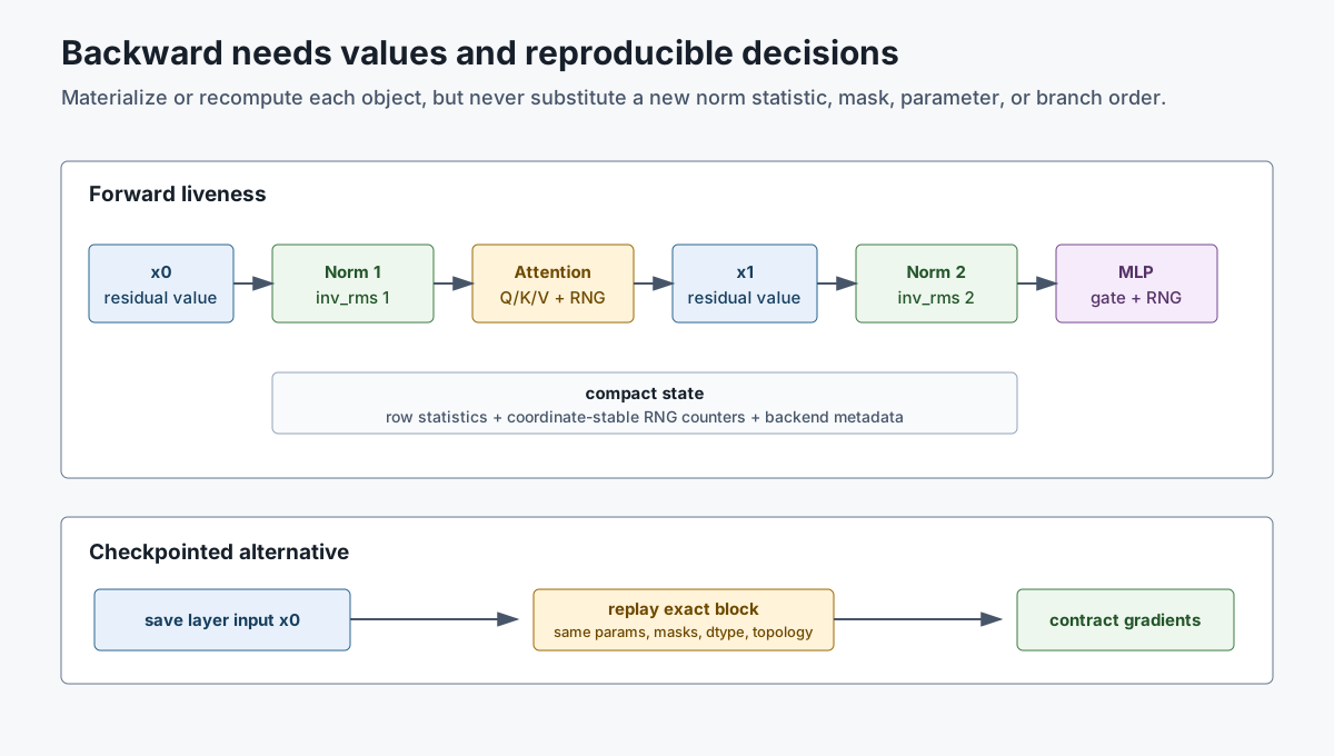
Recomputation contract

An activation-checkpointed block can save the layer input and replay the branches during backward, following the general compute-for-memory idea in Chen et al.. Exact replay additionally requires:

same parameters and buffers as the original forward
same norm family, axes, epsilon, and accumulation policy
same attention visibility and position state
same dropout logical random field
same train/eval flags and autocast policy
same branch order and parallel ownership

If an optimizer step or mutable buffer update occurs between forward and recompute, replaying from the new state is incorrect. Training systems normally finish backward before updating parameters for precisely this dependency.

In-place residual writes need a liveness proof

Code such as:

x += branch(norm(x))

can be wrong even when eager inference matches an out-of-place reference. Norm backward may need the pre-add x; branch backward may retain a view; autograd may track a version counter; checkpoint replay may expect the original layer input. Safe in-place execution requires proof that no consumer or saved view needs the overwritten value and that the framework’s alias rules allow it.

A compiler may still fuse the add without exposing an in-place source-level mutation. Fusion is a storage schedule; it does not relax value dependencies.

Encoder-decoder state ownership during backward

In the decoder cross-attention branch:

decoder state x:       receives residual update and decoder-side gradient
encoder memory m:      supplies K/V and receives gradient during joint training
cross-attention output target rows [B,T,D]: added only to decoder x

The encoder memory is not overwritten by the decoder residual add. During autoregressive inference it may be immutable and cached; during end-to-end training its gradient is accumulated through every decoder layer that reads it. This ownership distinction survives activation checkpointing.

Mixed precision

Moment reductions can overflow or lose precision if computed naively in FP16/BF16. Common kernels accumulate mean, variance, or mean-square in FP32 and cast the normalized result back to the input dtype. The learned weight may be stored in model dtype while the multiply uses promoted arithmetic.

def rmsnorm_reference(x, weight, eps):
    input_dtype = x.dtype
    x32 = x.float()
    inv_rms = torch.rsqrt(x32.square().mean(-1, keepdim=True) + eps)
    y = (x32 * inv_rms).to(input_dtype)
    return y * weight

Moving epsilon outside the square root, casting before the reduction, or using a different variance algorithm can create drift across hundreds of layers.

Fused residual-normalization kernels

The equations expose fusion opportunities:

Post-LN:
    add branch + residual
    reduce moments
    normalize and affine-transform

Pre-LN next branch:
    previous residual add
    reduce moments for next sublayer input

A kernel can combine residual addition, dropout, and normalization to avoid materializing an intermediate state in HBM. A valid fusion must preserve the unfused dataflow:

branch_with_bias = branch + optional_bias
dropped_branch = dropout(branch_with_bias, rng_identity)
residual_out = cast_to_residual_dtype(dropped_branch) + residual
normalized_out = norm(residual_out, eps, accumulation_dtype)

The two logical outputs are semantically different even though both have shape [B,S,d_model]. Passing normalized_out forward as the residual silently changes a Pre-LN stack. A fused ABI must additionally declare output order, whether it returns the pre-add residual or post-add residual, aliasing, saved state, RNG ownership, and output dtype. Tuple shape does not identify tuple meaning.

A hash-pinned Megatron-Core source trace

At Megatron-LM revision 23b2ff22eea5a150fec2b41b4d035afa216c8040, the bias-dropout-add helper accepts (branch, optional_bias), residual, dropout probability, and training mode. Its order is:

branch, bias = branch_with_bias
if bias is not None:
    branch = branch + bias
branch = dropout(branch, p=p, training=training)
output = residual + branch

If the branch and residual dtypes differ, the helper casts branch and bias to the residual dtype before the add. With fp32_residual_connection, the residual stream and output therefore stay FP32, and pipeline communication must use a compatible dtype. The implementation permits in-place mutation only in evaluation when branch, residual, and bias do not require gradients; that is a liveness condition, not merely a performance flag.

The same pinned Transformer layer accepts a normalization module that may return a tuple. Its expected order is exactly:

(normalized_output, residual)

The current Transformer-Engine adapter implements this for fused residual RMSNorm by forking the norm input with MakeExtraOutput, then applying RMSNorm. Here residual is the unnormalized input fork, not the result of a fused residual addition. The layer later feeds the first item to attention and keeps the second item for bias-dropout-add. This concrete ABI is the reverse of many informal (residual, normed) descriptions.

The optimized inference path is a third contract: Megatron can pass a residual into an attention output projection that fuses tensor-parallel reduce-scatter, residual add, layer normalization, and all-gather. That path does not prove the same fusion is active during training, with bias, or with dropout.

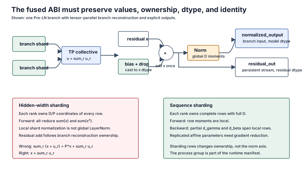
Fusion admission and parity

Semantic parity is tested against the unfused graph under one manifest:

Field	Must match
branch bias	absent/present and broadcast axis
dropout	probability, training mode, mask/RNG identity, scaling convention
residual	pre-add value, ownership, dtype, aliasing permission
norm	LayerNorm/RMSNorm family, epsilon, affine state, reduction axis
numerics	accumulation dtype, variance algorithm, output cast
outputs	tuple arity/order, pre-add vs post-add residual, aliasing
backward	saved/recomputed statistics, dropout replay, affine-gradient reductions

allclose tolerances may be appropriate when two kernels use different legal reduction orders. Bitwise equality should not be promised without matching the reduction tree and arithmetic mode. Performance belongs to M4; M3.7’s gate is semantic and checkpoint compatibility.

Distributed execution

Tensor-parallel attention and MLP branches often all-reduce or reduce-scatter their model-width outputs before the residual add. The residual state may be replicated, sequence-sharded, or context-parallel depending on the system. The addition is valid only when both operands have the same ownership map, not just the same local shape.

LayerNorm/RMSNorm reduce across d_model. If tensor parallelism shards that feature axis, a mathematically global norm requires cross-rank sums for

$$\sum_r x_r, \qquad \sum_r x_r^2.$$

Many Transformer tensor-parallel layouts keep each residual row’s full hidden width replicated at norm boundaries precisely to avoid or control this reduction. Sequence parallelism can shard rows instead because each row’s statistics are independent, but affine-parameter gradients still need reduction across ranks during training.

The distinction is easiest to state by ownership:

Layout at norm boundary	Local tensor	Forward moment collective	Affine-gradient collective
replicated hidden rows	[S_local,B,D] on each TP rank	none for norm; replicated computation	reduction follows parameter-replica policy
sequence parallel	disjoint rows [S/P,B,D], full D	none: every row is complete	sum d_gamma/d_beta across row-owning ranks
hidden-width sharded	same rows, local D/P	all-reduce row sum and square sum; LayerNorm also needs global mean	shard/replica policy plus any needed row reduction
context parallel	sequence ownership depends on the runtime’s exchange schedule	row-local norm needs no statistic exchange once each row is locally complete	reduce replicated affine gradients across owners

For hidden-width sharding with global width $D=\sum_r D_r$, LayerNorm needs

$$\mu=\frac{1}{D}\sum_r\sum_{j=1}^{D_r}x_{r,j},$$ $$\sigma^2=\frac{1}{D}\sum_r\sum_{j=1}^{D_r}x_{r,j}^2-\mu^2.$$

Computing one local mean and variance per shard and concatenating normalized pieces is wrong because each shard uses a different denominator. RMSNorm drops the first sum but still needs the global square sum.

Sequence parallelism avoids that forward collective only because it shards rows, not the normalized feature axis. During backward, each rank computes partial affine gradients

$$d\gamma_r=\sum_{(b,s)\in\mathcal R_r}g_{b,s}\odot\hat x_{b,s}, \qquad d\beta_r=\sum_{(b,s)\in\mathcal R_r}g_{b,s},$$

and replicated norm parameters require $\sum_r d\gamma_r$ and $\sum_r d\beta_r$ before the optimizer update.

Tensor-parallel branch outputs introduce a separate ownership rule. If $u=\sum_r u_r$ is reconstructed by an all-reduce, the residual must be added once:

$$y=x+\sum_r u_r.$$

Summing rank-local values x + u_r would produce $Px+u$ and multiply the shortcut by the TP degree. A reduce-scatter/add fusion is valid only when its output shard map matches the next residual owner.

Runtime integration checklist

before launch:
    validate norm family, epsilon, affine keys, residual dtype
    validate row/hidden ownership and process groups
    validate fused tuple ABI and in-place eligibility
    select deterministic dropout/recompute policy

after launch:
    compare unfused and fused intermediate tensors
    compare hidden-sharded global moments with a full-width oracle
    compare summed affine gradients with the unsharded reference
    assert residual is added once after TP branch reconstruction

The pinned Megatron source passes sequence_parallel into its Transformer Engine norm constructor and marks duplicated parameters for the appropriate gradient reductions. Those flags are runtime ownership metadata; they do not change LayerNorm’s mathematical axis.

Block conformance test

Shape tests are insufficient. Compare intermediate semantics against a reference:

with torch.no_grad():
    ref_norm = reference.input_layernorm(x)
    ref_attn = reference.self_attn(ref_norm, ...)[0]
    ref_h = x + ref_attn
    ref_mlp_norm = reference.post_attention_layernorm(ref_h)
    ref_mlp = reference.mlp(ref_mlp_norm)
    ref_y = ref_h + ref_mlp

    cand_y, trace = candidate(x, return_trace=True)

torch.testing.assert_close(trace.attn_norm, ref_norm)
torch.testing.assert_close(trace.after_attn_residual, ref_h)
torch.testing.assert_close(trace.mlp_norm, ref_mlp_norm)
torch.testing.assert_close(cand_y, ref_y)

This localizes whether drift begins at normalization, the branch, residual addition, or final state.

---

0x0B What block assembly does not own

M3.7 uses attention and MLP calls without reopening their internals:

M3.1:
    scores -> mask -> softmax -> value mix

M3.2:
    Q/K/V projections -> head split -> attention -> merge -> W_O

M3.6:
    dense FFN or gated MLP channel transformation

M3.7:
    norm -> sublayer -> branch dropout -> residual update

It also stops before downstream concerns:

[M3.8](/posts/m3-8-output-head-logit-interface):
    final hidden rows -> vocabulary logits

M4.1:
    integrated block/model totals, HBM traffic, arithmetic intensity

M5.1:
    persistent request/KV-cache lifecycle and publication

M5.2:
    multi-request scheduling and preemption policy

M5.3:
    physical cache allocation, mapping, reference ownership, and copy-on-write

Normalization placement affects training behavior, so M3.7 compares the major scaling variants and their contracts. It does not convert those source-reported methods into interchangeable patches for an existing checkpoint.

---

0x0C Shape ledger

Shared block objects

Object	Shape	Meaning
residual state x	[B,S,d_model]	Persistent model-width state rows.
norm mean	[B,S,1]	LayerNorm only; mean over features.
norm variance / mean square	[B,S,1]	LayerNorm variance or RMSNorm mean square.
norm scale gamma	[d_model]	Per-feature learned scale.
LayerNorm bias beta	[d_model]	Per-feature learned shift.
normalized state	[B,S,d_model]	Same shape as input.
attention branch output	[B,S,d_model]	Must be merged and output-projected.
MLP branch output	[B,S,d_model]	Must be contracted from d_ff.
dropped branch update	[B,S,d_model]	Branch tensor before residual add.
updated residual state	[B,S,d_model]	Input to the next branch or layer.
final normalized state	[B,S,d_model]	Input to the output head in Pre-LN stacks.

Block equations

Contract	Attention update	MLP update
Post-LN	h = Norm1(x + Dropout(Attn(x)))	y = Norm2(h + Dropout(MLP(h)))
Pre-LN	h = x + Dropout(Attn(Norm1(x)))	y = h + Dropout(MLP(Norm2(h)))
LLaMA-style	h = x + Attn(RMSNorm1(x))	y = h + MLP(RMSNorm2(h))

Encoder-decoder decoder objects

Object	Shape	Residual owner
decoder state x	[B,T,d_model]	Persistent target-side state.
encoder memory m	[B,S,d_model]	Read by cross-attention; not directly added.
masked self-attn output	[B,T,d_model]	Added to decoder state.
cross-attn output	[B,T,d_model]	Query-indexed; added to decoder state.
decoder MLP output	[B,T,d_model]	Added to decoder state.

---

0x0CA Evaluation, migration, release, and rollback

A block rewrite is not validated when one final tensor is close on one random input. Residual and normalization errors can cancel at the output while the intermediate state, saved backward values, or distributed ownership is already wrong. The release unit is the complete block contract recorded in 0x01.

Conformance matrix

Gate	Inputs and modes	What must match	Why final-output parity is insufficient
formula oracle	constant, zero-variance, shifted, scaled, and adversarial rows	moments, inverse denominator, normalized row, affine output	catches wrong axes, epsilon placement, and variance correction
eager forward	multiple shapes, masks, and sequence lengths	every norm input/output, branch output, residual add, and final norm	localizes the first divergent operator
backward	scalar loss plus direct vector-Jacobian products	input, affine, branch, and tied-parameter gradients	forward-compatible rewrites can have a wrong saved-state/backward path
finite difference	small FP64 fixtures away from nondifferentiable points	selected input and parameter derivatives	audits hand-derived or fused backward equations
mixed precision	FP32 reference versus BF16/FP16 policy	work dtype, output dtype, finite values, tolerance envelope	moment accumulation and residual dtype can diverge independently
dropout replay	fixed RNG identity, train/eval, checkpoint on/off	mask identity and gradients	equal probability does not reproduce the same stochastic function
fused path	eager versus every admitted fused ABI	tuple order, residual output, normalized output, gradients	identical shapes can name different outputs
distributed path	unsharded versus sequence/hidden/tensor-parallel fixtures	global moments, affine-gradient reductions, one residual add	local statistics and duplicated shortcuts can look plausible per rank
checkpoint round trip	save, load, resume, and export	key set, aliases, buffers, optimizer state, schedule counters	state-dict shape checks omit topology and mutable lifecycle state
training smoke	short deterministic run from the declared initialization	loss finiteness, update ratios, gradient profile, resume parity	initialization methods are training recipes, not static functions
inference canary	prompt/output corpus or task fixture	logits/hidden states, latency envelope, memory, error counters	operational regressions need real backend and serving state

Tolerance is a declared policy, not allclose by habit. FP32 algebraic oracles can demand near-machine precision. Mixed-precision kernels need absolute and relative tolerances justified against an FP32 reference, plus explicit NaN/Inf rejection. Stochastic comparisons either replay identical randomness or compare a predeclared statistical property over enough samples; they must not mix the two contracts.

Method-specific evaluation state

Architecture	Extra measurements required before release
Post-/Pre-/Peri-LN	per-site input/output RMS, residual/update ratio, first divergent layer, final-norm presence
ReZero / LayerScale	gate values and gradients by layer/channel; branch parameters must receive gradients once gates open
Fixup / T-Fixup / DeepNorm / DeepScaleLM	exact matrix-group initialization statistics, depth constants, warmup/regularization recipe, gradient profile by depth
Admin	profile dataset identity, profiled moments, computed shortcut vectors, post-reinitialization checkpoint hash
NormFormer	every extra norm/head-scale key and site; compute-matched baseline metadata
RealFormer	score-state norm/entropy by layer and attention family; running-sum/mean policy; transient-state shape
nGPT	hidden-row norm error, parameter-vector norm error after every step, eigen-rate ranges, q/k and logit scales
DyT	alpha by site, input range, saturation fraction, derivative distribution, post-embedding scalar
PRepBN	transition step and gamma, running-stat age, calibration dataset, train/eval parity, fold error

Useful residual telemetry is directional as well as scalar. For state $x_l$ and update $u_l$, record

$$\rho_l=\frac{\operatorname{RMS}(u_l)} {\operatorname{RMS}(x_l)+\delta}, \qquad c_l=\frac{\langle x_l,u_l\rangle} {\|x_l\|_2\|u_l\|_2+\delta}.$$

The ratio shows update scale; cosine alignment distinguishes reinforcement from rotation or cancellation. Aggregate both over tokens and retain quantiles so a small population of unstable rows is not hidden by one mean.

Migration is a transaction

A topology or normalization change should proceed through explicit artifacts:

1. freeze source checkpoint + configuration + tokenizer/data fixture
2. emit immutable source manifest and cryptographic hashes
3. construct the candidate graph from a reviewed migration map
4. migrate parameters, aliases, buffers, and optimizer state where defined
5. initialize genuinely new state under the paper's contract
6. run formula, forward, backward, dtype, fusion, and distributed gates
7. run training/resume smoke tests when the method changes optimization
8. calibrate mutable statistics when the method requires them
9. export candidate + conversion report + rollback pointer
10. canary under explicit quality, latency, memory, and error thresholds

Some migrations intentionally cannot preserve the old function. Pre-LN to Post-LN, RMSNorm to DyT, baseline GPT to nGPT, and ordinary attention to RealFormer all alter the graph. Their release contract is then retraining or continued-training evidence, not a fabricated zero-error conversion claim.

Immutable release manifest

At minimum, record:

architecture:
  branch_order: [self_attention, mlp]
  topology: pre_rmsnorm
  final_norm: true
normalization:
  family: rmsnorm
  axes: [d_model]
  epsilon: 1.0e-6
  work_dtype: float32
residual:
  dtype: float32
  dropout_probability: 0.0
  scaling_recipe: baseline
runtime:
  eager_reference: pinned
  fused_abi: named_outputs
  parallel_layout: declared
state:
  checkpoint_hash: required
  optimizer_hash: required_for_resume
  rng_and_schedule_counters: required_for_resume
evidence:
  conversion_report: required
  conformance_report: required
  calibration_report: conditional
rollback:
  previous_artifact_hash: required
  trigger_thresholds: required

An architecture name alone is insufficient. The epsilon, final norm, residual dtype, dropout semantics, depth recipe, projection/calibration schedule, fused ABI, and parallel ownership all select a function or state lifecycle.

Canary and rollback

The canary compares a pinned previous artifact with the candidate on the same input corpus and runtime class. Promotion requires every hard correctness gate and all declared service thresholds. Rollback triggers include non-finite activations, conformance drift beyond tolerance, loss or quality regression, latency/memory envelope failure, rising saturation or residual-update ratios, invalid PRepBN statistics, and resume divergence.

Rollback means restoring the previous complete artifact: graph, checkpoint, tokenizer/configuration, runtime backend, calibration buffers, and scheduler state. Reusing candidate optimizer moments or running statistics with the old graph is not rollback.

Publish gate

• Every formula has a named oracle or a primary-source derivation.
• Every topology and paper variant has graph, initialization, training, inference, and checkpoint state stated explicitly.
• Eager, fused, mixed-precision, and distributed contracts are separated.
• Stochastic replay and recomputation preserve RNG identity.
• Source-reported empirical results remain scoped to their setup.
• Every visual has provenance and a semantic purpose.
• Migration, calibration, canary, and rollback artifacts are immutable.
• Neighboring M3/M4/M5 ownership is not duplicated.

---

0x0D Failure lab

Residual-shape and ownership bugs

1. Adding an unmerged attention tensor to the residual stream. [B,h,S,d_head] must be merged and projected to [B,S,d_model] first.

2. Adding an MLP intermediate to the residual stream. [B,S,d_ff] must pass through the down projection before addition.

3. Concatenating instead of adding. Width grows and the next layer no longer receives the checkpoint’s d_model contract.

4. Adding encoder memory directly to decoder state. Cross-attention returns a target-indexed [B,T,d_model] update; memory remains [B,S,d_model].

5. Treating residual addition as the source of causal leakage. The identity path contains the current row state. Future visibility is controlled inside masked attention before the residual add.

Normalization-axis and formula bugs

6. Normalizing over the sequence axis. LayerNorm(d_model) reduces the last feature axis for every token row, not S.

7. Normalizing over the batch axis. This changes behavior with batch composition and is not Transformer LayerNorm.

8. Treating the full sentence as one LayerNorm sample. Statistics should have shape [B,S,1], not [B,1,1] for the standard row-wise contract.

9. Implementing std + eps while claiming exact nn.LayerNorm. PyTorch uses sqrt(var + eps) with biased variance.

10. Using the wrong variance correction. Small feature widths can make the numerical difference visible even though shapes match.

11. Computing low-precision variance without the checkpoint implementation’s cast. LLaMA RMSNorm computes the mean square in float32 before casting back.

12. Using a mismatched epsilon. 1e-5, 1e-6, and other values preserve shape but change normalization.

Norm-family and ordering bugs

13. Loading LayerNorm behavior under RMSNorm weights. Centering and bias semantics differ.

14. Adding a bias to a scale-only RMSNorm checkpoint. This silently changes the model function.

15. Moving a Post-LN checkpoint to Pre-LN because the tensor shapes still fit. The ordering is part of the architecture.

16. Reading post_attention_layernorm as Post-LN. In LLaMA it is applied before the MLP branch.

17. Sharing one norm instance across attention and MLP branches unintentionally. Parameter shapes match, but learned scales and biases become tied.

18. Omitting the final norm in a Pre-LN stack. The output head receives an unnormalized last residual state.

Dropout and branch bugs

19. Dropping the identity path. Standard wrappers apply dropout to the branch update before adding the unchanged residual.

20. Applying residual-branch dropout after the add. This can erase identity-state components and is not the Harvard or original Transformer contract.

21. Assuming attention dropout and residual dropout are one setting. They act on different tensors at different points.

22. Adding Harvard branch dropout to a checkpoint whose block omits it. Architecture code, not tutorial symmetry, is authoritative.

23. Leaving dropout active during evaluation. Block outputs become stochastic when deterministic evaluation is expected.

Assembly and boundary bugs

24. Changing decoder branch order. The encoder-decoder source uses masked self-attention, then cross-attention, then MLP.

25. Adding cross-attention to a decoder-only checkpoint. This introduces parameters and a memory input absent from the architecture.

26. Using different normalized inputs for Q, K, and V in self-attention. The Harvard Pre-LN call binds one normalized state as all three self-attention inputs. Cross-attention is the case where query and key/value sources differ.

27. Assuming Pre-LN guarantees better final quality. It changes optimization behavior; quality still depends on the full architecture and training recipe.

28. Claiming the residual path leaves the gradient unchanged. The identity term is one contribution; the branch Jacobian and the products across later layers still affect the total gradient.

29. Turning a local Jacobian identity into a universal Pre-LN quality claim. The equations distinguish gradient routes. They do not rank every architecture, depth, initialization, optimizer, or training recipe.

30. Treating a conceptual read/write ledger as an exact kernel trace. M3.7 counts local state, reductions, additions, and conceptual movement. M4.1 integrates the block and model totals; backend inspection is still required to determine fusion and actual HBM traffic.

31. Calling training degradation a synonym for vanishing gradients. A deeper plain network can have higher training error even when gradient underflow is not the sole cause; residual parameterization addresses optimization of identity-like mappings more broadly.

32. Scaling or dropping the shortcut while still calling it an identity path. Constant scaling, gates, projections, and DropPath all change the direct Jacobian.

33. Using the decoder-only DeepNorm constants for an encoder-decoder. The paper’s $\alpha$ and $\beta$ depend on architecture and depth definitions.

34. Replacing LayerNorm with RMSNorm or DyT after training. Equal input/output shapes do not preserve centering, scale invariance, saturation, learned parameters, or checkpoint behavior.

35. Treating RealFormer’s score residual as the hidden-state residual. The former carries [B,h,S,S] logits; the latter carries [B,S,d_model] state.

36. Normalizing a feature-sharded tensor locally when the contract requires global d_model statistics. Local moments differ from moments over the full hidden row unless cross-rank sums are performed.

37. Confusing a fused kernel’s normalized output with its residual output. Some APIs return both tensors with identical shapes and different meanings.

38. Letting padded rows enter a batch-coupled normalization estimate without an explicit policy. Valid-token outputs can then depend on padding and batch composition.

39. Assuming epsilon matters only for zero-variance rows. Epsilon also changes scale and gradients for any row whose variance or mean square is near its magnitude.

40. Verifying only final block output. Intermediate conformance checks localize whether drift starts at the first norm, attention update, residual add, second norm, or MLP update.

Depth-recipe and alternative-architecture bugs

41. Copying one depth exponent and calling it Fixup or T-Fixup. The matrix groups, zeroed layers, scalar/bias state, norm removal, optimizer, warmup, and regularization choices are part of the recipe.

42. Using Admin without the profile-and-reinitialize pass. Its shortcut vectors depend on measured branch statistics; an arbitrary constant is a different method.

43. Applying one DeepNorm constant to every architecture. Encoder-only, decoder-only, and encoder-decoder contracts use different depth and branch-count formulas.

44. Implementing NormFormer with one post-attention norm. The source recipe also changes head scaling and the FFN internal norm graph.

45. Deleting RMSNorm from a trained checkpoint and calling the result nGPT. nGPT changes residual updates, parameter constraints, attention/MLP scales, logits, optimizer regularization, and warmup.

46. Sharing one RealFormer score route across attention families. Encoder self-attention, decoder self-attention, and cross-attention have different axes, masks, and lifecycle identities.

47. Persisting RealFormer score state as a second generation-history cache. The score route travels across layer depth for the current forward/query row; K/V owns history across decode steps.

48. Using DyT’s generic alpha initialization for every LLM site. The paper reports width- and location-dependent LLM initialization plus a post-embedding scale.

49. Calling aggregate LayerNorm S-curves an elementwise identity. For one fixed row, LayerNorm couples coordinates through shared moments; the paper’s S-curves pool many rows.

50. Folding PRepBN before the transition or without refreshed statistics. The fixed-statistics algebra can be exact while the estimated running statistics are stale or invalid.

Release and runtime bugs

51. Accepting a fused kernel because final output matches once. Tuple identity, saved backward state, residual dtype, dropout replay, and gradients require separate checks.

52. Adding the residual independently on every tensor-parallel rank. If branch partials are summed afterward, the shortcut is multiplied by world size.

53. Loading weights but not aliases, mutable buffers, or schedule counters. Tied parameters, running statistics, dropout/recompute RNG, and progressive transitions can silently diverge.

54. Canarying a conversion without the previous complete artifact. A rollback pointer to weights alone cannot restore graph, runtime, calibration, and resume state.

55. Treating source-reported benchmark gains as release thresholds. A production gate must be measured on the target architecture, data, hardware, backend, and service objective.

---

0x0E Handoff to the output interface

M3.1 through M3.7 now define one full state-update path:

X_l: [B,S,d_model]
    -> normalized attention residual update
    -> normalized MLP residual update
X_{l+1}: [B,S,d_model]

After the final block and final normalization:

H_final: [B,S,d_model]

Those rows are still hidden states, not token probabilities or token IDs. M3.8 opens the next local interface:

final hidden row or matrix
    -> vocabulary projection
    -> logits / log-probabilities

M3.8 also consumes one [B,vocab_size] score row with a decoding policy, while M3.10 owns the single-request autoregressive transition. M5.1 owns persistent request/cache publication and lifecycle, M5.2 owns multi-request scheduling, and M5.3 owns physical cache allocation and mutation.

---

0xFF References

• Exploring the Transformer Series (14) — Residual Networks and Normalization
• M3.1 — Scaled Dot-Product Attention
• M3.2 — Multi-Head Attention Layout
• M3.6 — Dense and Gated MLPs
• M3.8 — Output Head and Decoding Policy
• M4.1 — Transformer Cost Model
• Vaswani et al., Attention Is All You Need
• Ba et al., Layer Normalization
• Zhang and Sennrich, Root Mean Square Layer Normalization
• Xiong et al., On Layer Normalization in the Transformer Architecture
• Liu et al., Understanding the Difficulty of Training Transformers
• Wang et al., DeepNet: Scaling Transformers to 1,000 Layers
• Nguyen and Salazar, Transformers without Tears: Improving the Normalization of Self-Attention
• Shleifer et al., NormFormer: Improved Transformer Pretraining with Extra Normalization
• He et al., RealFormer: Transformer Likes Residual Attention
• Loshchilov et al., nGPT: Normalized Transformer with Representation Learning on the Hypersphere
• Zhu et al., Transformers without Normalization
• Guo et al., SLAB: Efficient Transformers with Simplified Linear Attention and Progressive Re-parameterized Batch Normalization
• Srivastava et al., Dropout: A Simple Way to Prevent Neural Networks from Overfitting
• Srivastava et al., Highway Networks
• He et al., Deep Residual Learning for Image Recognition
• He et al., Identity Mappings in Deep Residual Networks
• Orhan and Pitkow, Skip Connections Eliminate Singularities
• Bachlechner et al., ReZero is All You Need
• Zhang et al., Fixup Initialization
• Huang et al., T-Fixup: Training Transformers without Layer Normalization
• Touvron et al., Going Deeper with Image Transformers
• Kedia et al., Transformers Get Stable
• Shen et al., PowerNorm
• Huang et al., Deep Networks with Stochastic Depth
• Chen et al., Training Deep Nets with Sublinear Memory Cost
• Chowdhery et al., PaLM
• Kim et al., Peri-LN
• PyTorch 2.13, torch.nn.LayerNorm
• Hugging Face Transformers v5.13.1 at revision 4626421, LlamaDecoderLayer and LlamaRMSNorm
• NVIDIA Megatron-LM 23b2ff22, TransformerLayer, fused_bias_dropout, and Transformer Engine adapters