M3.9 — Training Execution: Teacher Forcing, Masks, Loss, and Parallelism
0x00 Overview And Background
There is a sentence that is easy to remember and easy to misunderstand:
Transformer training is parallel.
If we read it too quickly, it sounds as if training has stopped being autoregressive. That is not the case. The supervised objective is still a next-token objective:
p(y | x) = product_t p(y_t | y_<t, x)
For encoder-decoder training, the decoder row that predicts y_t should only use the source sequence and the previous target tokens y_<t. What changes during training is not the probability factorization. What changes is that the full gold target sentence is already available in the dataset. The code can therefore build all gold prefixes in one rectangular tensor, use a causal mask to prevent future leakage, and compute many target-position losses in one forward pass.
The local code path is:
for i, batch in enumerate(data_iter):
    out = model.forward(batch.src, batch.tgt, batch.src_mask, batch.tgt_mask)
    loss, loss_node = loss_compute(out, batch.tgt_y, batch.ntokens)
This is the part M3.9 owns. M3.1–M3.8 established the computation from masked attention through the output head. Here we study the training loop around those objects:
collate / Batch
    -> src, tgt, tgt_y, src_mask, tgt_mask, ntokens
        -> model.forward(...)
            -> decoder hidden states out
                -> SimpleLossCompute
                    -> generator(out)
                        -> flatten predictions and labels
                            -> admitted local criterion
                                -> additive numerator + denominator
                                    -> one backward seed
                                        -> distributed completion + one-time unscale
                                            -> finite agreement + one global clip
                                                -> optimizer / scheduler commit
The short version is:
training is parallel in tensor computation,
but autoregressive in the visibility rule and loss objective.
The rest of this article follows the objects that make this possible.
Owner question
How does a corpus become correctly shifted and masked supervised rows, and how do those rows turn into numerically stable gradients, distributed updates, and restartable training state without changing the autoregressive objective?
M3.9 owns the training-side semantic transaction. It defines the supervised rows, objective reduction, logical update, and restart requirements; it does not claim that a particular distributed backend, checkpoint store, converted artifact, or live release executed successfully:
examples -> token/segment metadata -> batches or packed streams
inputs + query/key visibility + target/loss ownership
forward -> admitted head/criterion -> additive objective -> one backward seed
complete declared gradient collectives + unique-owner/denominator readiness
-> one-time unscale -> finite agreement -> one binary32 global norm and clip
-> selected logical update -> bounded physical projection -> durable checkpoint
evaluation requirements -> later-owner artifact and release handoff
It does not reopen tokenizer learning (M2.1), initial embedding/model-width state (M2.2), block equations (M3.1–M3.8), single-request generation (M3.10), live scheduling/session/cache behavior (M5), physical artifact conversion and runtime admission (M8.9), or deployment promotion, monitoring, rollback, and release (M8.10).
Evidence and implementation boundary. Equations in this article state technical contracts. Pinned source excerpts describe those exact historical revisions. Pseudocode and finite fixtures are reference models, not evidence that a framework, distributed job, checkpoint store, evaluation, serving artifact, canary, or rollback ran. Whenever a later section compresses the transaction, this owner boundary and the typed contracts take precedence.
How the training contract reached this form
The phrase teacher forcing came from recurrent-network training. In a free-running recurrent decoder, the output produced at step becomes an input at step . During teacher-forced training, the known target from the dataset is supplied instead. The distinction was therefore originally a choice inside a sequential recurrence:
free-running recurrence:
    input at t <- model output sampled at t-1

teacher-forced recurrence:
    input at t <- gold target token at t-1
The source-series comparison below makes that replacement visible. Read the right-hand path as a training-input policy, not as permission to expose the future target. Each prediction still receives only the preceding gold target.
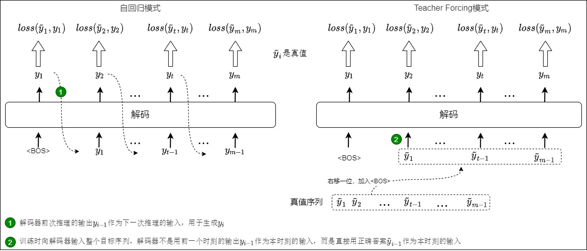
t, free running consumes the model token selected at t-1; teacher forcing consumes gold token y_(t-1). In both cases the model predicts y_t.Recurrent sequence-to-sequence systems retained this stepwise schedule even when every gold target was known. The Transformer changed the materialized schedule. Its masked self-attention has no recurrent edge between neighboring decoder rows, so all shifted gold inputs can be embedded and processed in one tensor call while the causal mask preserves the same conditional support. This is why the 2017 Transformer paper could describe a model that remained autoregressive while being substantially more parallelizable during training.
Modern decoder-only pretraining and supervised fine-tuning did not remove that contract. They widened it:
recurrent teacher forcing:
    gold previous token -> one sequential decoder step

Transformer teacher forcing:
    all gold previous-token rows -> one causally masked tensor schedule

packed pretraining:
    many document segments -> one physical stream + segment-safe visibility

instruction tuning:
    one chat-template stream -> causal visibility + assistant-target ownership

distributed training:
    many local token sums -> one declared global objective and update
The last two lines are not cosmetic batching changes. They add new identities:
segment boundaries, position resets, supervised spans, global denominators,
collective order, optimizer ownership, and restart state. M3.9 therefore cannot
stop at loss.backward(). Its subject is the complete update transaction.
| Claim | Status | Evidence boundary |
|---|---|---|
| teacher forcing feeds known targets instead of prior model outputs during training | externally verified | Williams and Zipser’s recurrent training procedure; A5’s source-local reconstruction |
| a Transformer remains autoregressive while masked target rows can execute in parallel | externally verified | Attention Is All You Need and the Annotated Transformer |
| packing can be equivalent only when examples cannot contaminate one another | externally verified | Efficient Sequence Packing without Cross-contamination |
| modern SFT needs a separate target-ownership policy over the serialized chat stream | official implementation boundary | Hugging Face chat-template and TRL SFT contracts; exact behavior is template/version specific |
| distributed training preserves one objective only when numerator, denominator, and reduction conventions agree | derivation in this article | objective, accumulation, and distributed-reduction algebra plus executable oracles |
Ownership firewall
| M3.9 consumes | M3.9 owns | M3.9 defers |
|---|---|---|
| M2.1 token IDs, special-token policy, collated rows, and segment metadata | shifted input/target addresses, visibility construction, loss ownership, reduction, backward, update, and restart state | tokenizer learning, vocabulary construction, and generic collation algorithms remain in M2.1 |
| M3.1 attention-mask semantics and M3.8 vocabulary score rows | which training rows exist, which rows are supervised, and how their gradients form one update | attention kernel semantics remain in M3.1; head geometry and local score policy remain in M3.8 |
| model parameters and logical block interfaces | accumulation, precision, parallel ownership, optimizer/scheduler transition, and checkpoint/evaluation requirements | physical FLOPs, traffic, kernels, and hardware efficiency remain in M4 |
| a declared training objective | exact/statistical restart classification and the logical handoff requirements for later artifacts | inference iteration remains in M3.10; live scheduling/session/cache lifecycle in M5; distillation in M6.10; speculative execution in M7; physical artifact admission in M8.9; deployment evaluation, canary, promotion, monitoring, rollback, and release in M8.10 |
Background knowledge: factorization is not an execution schedule
Teacher forcing predates the Transformer. Recurrent encoder-decoder models also trained by feeding the gold previous target while asking the model to predict the next one. The Transformer changes the schedule because causal masking lets all gold prefixes occupy one rectangular tensor:
probability model:
    still factorized left to right

training data:
    supplies every gold prefix simultaneously

causal mask:
    prevents row t from reading labels after t

loss mask:
    decides which predicted rows contribute to optimization
Parallel training therefore means parallel evaluation of conditionally valid rows. It does not mean the model is allowed to condition on future target tokens, and it does not make attention masks interchangeable with padding or loss masks.
0x01 The Code Object: run_epoch
The best place to start is not an abstract definition of teacher forcing. It is
the training loop. The next listing is a pinned historical source specimen and
navigation aid, not the denominator-safe, successful-update, checkpointable
reference transaction developed later. In the Harvard / Annotated Transformer
revision cited below, run_epoch() receives an iterable of Batch objects, the
model, a loss-compute object, an optimizer, and a scheduler:
def run_epoch(
    data_iter,
    model,
    loss_compute,
    optimizer,
    scheduler,
    mode="train",
    accum_iter=1,
    train_state=TrainState(),
):
    total_tokens = 0
    total_loss = 0
    tokens = 0
    n_accum = 0

    for i, batch in enumerate(data_iter):
        out = model.forward(
            batch.src, batch.tgt, batch.src_mask, batch.tgt_mask
        )

        loss, loss_node = loss_compute(out, batch.tgt_y, batch.ntokens)

        if mode == "train" or mode == "train+log":
            loss_node.backward()
            train_state.step += 1
            train_state.samples += batch.src.shape[0]
            train_state.tokens += batch.ntokens

            if i % accum_iter == 0:
                optimizer.step()
                optimizer.zero_grad(set_to_none=True)
                n_accum += 1
                train_state.accum_step += 1

            scheduler.step()

        total_loss += loss
        total_tokens += batch.ntokens
        tokens += batch.ntokens

        del loss
        del loss_node

    return total_loss / total_tokens, train_state
This loop names many objects used by the article, but it does not by itself define their cadence, denominator, update-success, precision, distributed, or checkpoint contracts:
batch.src:
    source token IDs

batch.tgt:
    shifted target input IDs

batch.tgt_y:
    next-token labels

batch.src_mask:
    source padding visibility

batch.tgt_mask:
    target padding + causal visibility

out:
    decoder hidden states, not vocabulary logits

loss_compute:
    generator + criterion + normalization

loss_node:
    differentiable scalar used by backward()

optimizer / scheduler:
    parameter update and learning-rate schedule
The current article should be read from this loop outward. Teacher forcing is not a magic training mode hidden inside the Transformer block. Precisely, it is the gold-prefix input policy: a training prediction row receives the known previous target rather than a model-generated token. Shifting, hard visibility, target ownership, loss reduction, and update execution are separate contracts that make the complete training transaction correct; they are not all synonyms for teacher forcing.
The following ledger is the object contract for the rest of the article:
| Object | Shape | Created by | Role |
|---|---|---|---|
| raw examples | list of source/target pairs | dataset iterator | unbatched training samples |
src | [B, S] | collate_batch | padded source token IDs |
| full target | [B, T_full] | collate_batch | padded target token IDs before shift |
batch.src | [B, S] | Batch.__init__ | source IDs passed to model.forward |
batch.src_mask | [B, 1, S] | (src != pad).unsqueeze(-2) | source padding visibility |
batch.tgt | [B, T_full - 1] | tgt[:, :-1] | decoder input IDs, gold prefix side |
batch.tgt_y | [B, T_full - 1] | tgt[:, 1:] | next-token labels, supervision side |
| target pad mask | [B, 1, T] | (tgt != pad).unsqueeze(-2) | hides padded target keys |
| future mask | [1, T, T] | subsequent_mask(T) | blocks target positions j > i |
batch.tgt_mask | [B, T, T] | make_std_mask | target padding plus causal visibility |
batch.ntokens | scalar | (tgt_y != pad).sum() | historical baseline count of non-PAD target labels; not the general eligible-row denominator |
out | [B, T, d_model] | model.forward(...) | decoder hidden states |
| generator output | [B, T, V_tgt] | generator(out) | vocabulary scores or log-probabilities |
| flat predictions | [B*T, V_tgt] | contiguous().view(-1, V_tgt) | one row per target position |
| flat labels | [B*T] | contiguous().view(-1) | one class index per target position |
true_dist | [B*T, V_tgt] | LabelSmoothing | smoothed target distribution |
loss_node | scalar tensor | criterion(...) / ntokens | graph-connected value for backprop |
This table is also a debugging map. When training breaks, the fastest question is not “is teacher forcing enabled?” It is:
for this row of out,
which target input positions were visible,
and which row of tgt_y is it compared against?
The immutable training manifest
The tensor table describes one batch. It does not identify the run that created the batch or the update transaction that will consume it. Two jobs can have identical tensor shapes and still optimize different objectives because they use different templates, pack boundaries differently, average different units, or advance the schedule on different counters.
A reproducible run therefore needs an immutable manifest before the first optimizer step. The useful split is:
immutable contract:
    what examples, rows, objective, update, and topology mean

mutable progress state:
    where this run currently is inside that contract
| Manifest namespace | Required identity | Why shape checks cannot recover it |
|---|---|---|
data | dataset revision/checksum, split, mixture weights, filtering/dedup policy, sample-address scheme | the same token shape can come from a different corpus or mixture |
representation | tokenizer hash, vocabulary size, special-token IDs, normalization, chat-template hash | equal IDs can name different token strings or roles |
batch | max length, padding side, truncation, packing algorithm, boundary-label policy, position reset, worker/sampler policy | all produce legal rectangular tensors with different supervision |
objective | factorization, shift owner, attention-mask family, target-owner rule, ignore ID, smoothing convention, weights, reduction denominator | the scalar can look plausible while weighting rows differently |
update | accumulation unit/window, optimizer type and groups, weight decay, clip rule, scheduler family and step unit | the same gradient can produce a different transition |
numerics | parameter/compute/reduction dtype, autocast policy, loss-scaling policy, finite-check order, deterministic policy | dtype names alone do not describe where conversion occurs |
parallel | DP/TP/PP/SP/CP/ZeRO degrees, rank map, collective semantics, pipeline schedule | world size alone does not identify state ownership or reduction |
rng | named data/model/pipeline streams and derivation rule | one global seed does not reconstruct per-rank stochastic order |
checkpoint | shard schema, alias/tied-weight policy, saved state classes, version and migration policy | files can load while silently omitting optimizer or sampler state |
release | code revision, dependency/container/hardware contract, evaluation suite, acceptance thresholds, rollback target | a checkpoint is not a validated training release |
One compact manifest might contain:
{
  "schema_version": "m3.9-training-v1",
  "data": {
    "dataset_manifest_sha256": "...",
    "split": "train",
    "sample_address": "dataset/document/segment/token-offset",
    "mixture_weights": {"web": 0.7, "code": 0.3}
  },
  "representation": {
    "tokenizer_sha256": "...",
    "chat_template_sha256": "...",
    "bos_id": 1,
    "eos_id": 2,
    "pad_id": 0
  },
  "batch": {
    "max_tokens": 8192,
    "packing": "segment-safe",
    "cross_segment_target": "masked",
    "position_policy": "reset-per-segment"
  },
  "objective": {
    "family": "causal-next-token",
    "shift_owner": "external-collator",
    "loss_owner": "assistant-target-token",
    "reduction": "global-valid-token-mean",
    "label_smoothing": {"epsilon": 0.0, "support": "none"}
  },
  "update": {
    "accumulation": {"unit": "microbatch", "count": 8},
    "optimizer": "AdamW",
    "parameter_group_sha256": "...",
    "clip": {"kind": "global-l2", "max_norm": 1.0},
    "scheduler": {"family": "cosine", "step_unit": "successful-update"}
  },
  "numerics": {
    "parameter_dtype": "bf16",
    "reduction_dtype": "fp32",
    "loss_scaling": "disabled-for-bf16"
  },
  "parallel": {"dp": 8, "tp": 2, "pp": 2, "sp": true, "zero_stage": 1},
  "rng": {"streams": ["data", "dropout", "pipeline"], "rank_derivation": "declared"}
}
The values above are an illustrative logical schema, not a closed serialized
manifest, a recommended universal configuration, or replay evidence. A real
immutable identity needs a deterministic serialization, its authenticated
payload bytes and digest, schema/version validation, and an explicit
classification of every absent or inapplicable field. The contract is the
explicitness. In particular,
step_unit="successful-update" means a skipped AMP update does not advance the
scheduler. A token-based schedule would instead declare a globally committed
token counter.
Mutable state belongs beside, but not inside, the immutable identity:
| Mutable state | Meaning |
|---|---|
microbatch_step | forward/backward transactions attempted |
successful_update_step | optimizer transitions actually committed |
global_valid_tokens | supervised denominator committed across ranks |
epoch and sampler cursor | next sample address and shuffle position |
| accumulation remainder | unstepped gradient window and its token denominator |
| optimizer moments and per-parameter step | update history |
| scheduler and scaler state | next learning rate and overflow policy |
| named RNG states | next data order, dropout mask, corruption, and pipeline stochastic event |
This separation creates three compatibility outcomes:
same immutable contract + same mutable state:
    exact-resume candidate under the declared software/hardware bound

same immutable contract + intentionally reset mutable state:
    warm start or new run, never mislabeled exact resume

different immutable objective/data/update identity:
    migration or new experiment requiring an explicit compatibility decision
An immutable manifest does not guarantee determinism. It makes divergence auditable: a reviewer can distinguish changed semantics from floating-point or runtime nondeterminism. Resolving a previously unspecified row, objective, parameter-group, precision, topology, or update field changes the immutable identity. Existing mutable progress must then be explicitly migrated and rebound to the new identity, or the result is a new run; it cannot be called an exact continuation merely because tensor shapes still match.
0x02 Before the Loop: collate_batch and Rectangular Tensors
The model cannot train on a list of Python strings. Before Batch exists, the
dataloader has already converted examples into padded tensors. This is not the
main tokenizer article; M2.1 owns tokenizer algorithms, vocabulary addresses,
special-token semantics, and generic collation construction. M2.2 owns the
initial model-width representation state and embedding/output-tie eligibility.
Here we only need the upstream fact that src and full target tensors are
rectangular under an authenticated M2.1 representation identity.
A simplified collation path is:
processed_src = torch.cat(
    [
        torch.tensor([bos_id]),
        torch.tensor(src_vocab(src_pipeline(_src))),
        torch.tensor([eos_id]),
    ],
    0,
)

processed_tgt = torch.cat(
    [
        torch.tensor([bos_id]),
        torch.tensor(tgt_vocab(tgt_pipeline(_tgt))),
        torch.tensor([eos_id]),
    ],
    0,
)

src_list.append(pad(processed_src, ...))
tgt_list.append(pad(processed_tgt, ...))

src = torch.stack(src_list)
tgt = torch.stack(tgt_list)
return src, tgt
The result is:
src:        [B, S]
full_tgt:   [B, T_full]
For example:
full target row 1:
    <bos> I ate an apple <eos>

full target row 2:
    <bos> I ate <eos> <pad> <pad>
The rectangular shape is necessary for efficient tensor computation, but it introduces artificial positions. Padding is not semantic content. Later, src_mask, tgt_mask, tgt_y, and ntokens exist because the code must distinguish real supervision from rectangular padding.
The training worker wraps collated examples like this:
(Batch(b[0], b[1], pad_idx) for b in train_dataloader)
So the next object to inspect is Batch.
0x03 Batch: The Training Contract Object
The Batch class is where the training example becomes the set of tensors consumed by the model and the loss:
class Batch:
    def __init__(self, src, tgt=None, pad=2):
        self.src = src
        self.src_mask = (src != pad).unsqueeze(-2)

        if tgt is not None:
            self.tgt = tgt[:, :-1]
            self.tgt_y = tgt[:, 1:]
            self.tgt_mask = self.make_std_mask(self.tgt, pad)
            self.ntokens = (self.tgt_y != pad).data.sum()

    @staticmethod
    def make_std_mask(tgt, pad):
        tgt_mask = (tgt != pad).unsqueeze(-2)
        tgt_mask = tgt_mask & subsequent_mask(tgt.size(-1)).type_as(
            tgt_mask.data
        )
        return tgt_mask
The source side is simple:
self.src:
    [B, S]

self.src_mask:
    [B, 1, S]
The source sequence is already available, so the source mask mainly hides padding positions. It does not create a causal future rule.
The target side is the key:
self.tgt = tgt[:, :-1]
self.tgt_y = tgt[:, 1:]
If the full target is:
<bos> I ate an apple <eos>
then:
batch.tgt:
    <bos> I ate an apple

batch.tgt_y:
    I ate an apple <eos>
The decoder receives batch.tgt. The loss compares the decoder output against batch.tgt_y.
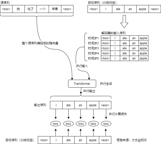
[BOS, I, ate, an, apple, EOS], decoder inputs omit EOS and labels omit BOS, so input row i predicts target i+1. Internal-shift APIs encode the same relation but must not be shifted a second time.[BOS, I, ate, an, apple]; aligned labels are [I, ate, an, apple, EOS]. Each pair retains its source/target address and still requires the eligibility and head-passport checks below.This is teacher forcing in code. At the row that predicts ate, the decoder input contains the gold prefix:
<bos> I
not a sampled previous output. The model can be wrong at one position while the next training row still receives the gold previous token. That is why training can build the whole target-side matrix at once.
Deriving the shifted rows from the factorization
The shift is not a framework convention that happened to become popular. It is the tensor form of the probability chain rule. For source and target ,
Introduce a start token . A teacher-forced decoder row indexed by consumes and represents the conditional state for target :
The causal visibility row is
The vocabulary head produces one score row , so the negative log-likelihood is
Every summand depends on a different allowed prefix, but there is no same-layer recurrent execution edge that requires row to finish before row begins. Rows may still depend on earlier token rows through the key/value states produced by earlier layers, as permitted by the attention support relation. The implementation can therefore materialize all , all mask rows , and all target addresses in one tensor schedule. Autoregression is in the support relation and in the factorization, not in a same-layer step-by-step recurrence.
Encoder-decoder and decoder-only training differ in where the conditioning source lives, not in this target-row relation:
| Training family | Conditioning state | Shifted prediction row |
|---|---|---|
| encoder-decoder | encoder states for all valid source tokens plus target prefix | decoder row predicts |
| decoder-only pretraining | same token stream prefix | residual row predicts |
| response-only SFT | serialized system/user/tool/assistant prefix | row predicts token , but contributes loss only when target owner |
| packed independent documents | same-segment causal prefix | physical row predicts the next same-segment token; cross-segment targets follow an explicit boundary policy |
One source address must survive every transformation
Flattening [B,T,V] to [B*T,V] later erases the visible batch/sequence axes.
An audit still needs to identify what each row means. Carry or reconstruct this
logical address:
target address:
    dataset revision
    example/document ID
    segment ID inside physical sequence
    logical target-token offset j
    physical batch row b and column t
    target token ID
    prediction-row address (b, t-1)
    attention-visibility descriptor
    loss-owner bit and optional row weight
For a packed decoder-only stream, let pi(s,j) map segment s and logical
offset j to physical column. Then the ordinary within-segment row relation is
Visibility also needs the segment equality:
At a physical boundary where , the naive next-token shift would create a cross-document pair. Independent-document packing normally sets that target row to the ignore ID; continuous-stream pretraining may deliberately retain it. Neither policy can be inferred from a lower-triangular mask.
A collator that preserves the address contract can make the separation explicit:
def materialize_rows(token_ids, segment_ids, target_owner, ignore_id=-100):
    input_ids = token_ids[:-1]
    labels = token_ids[1:].clone()

    input_segment = segment_ids[:-1]
    target_segment = segment_ids[1:]
    same_segment_target = input_segment == target_segment

    # Target ownership is defined on target tokens, then shifted to rows.
    row_owner = target_owner[1:] & same_segment_target
    labels[~row_owner] = ignore_id

    positions = reset_positions_within_each_segment(input_segment)
    visibility = (
        causal_relation(len(input_ids))
        & same_segment_matrix(input_segment)
    )

    row_address = build_row_address(
        input_ids=input_ids,
        labels=labels,
        segments=input_segment,
        positions=positions,
        row_owner=row_owner,
    )
    return input_ids, labels, positions, visibility, row_address
This particular pseudocode is the independent-document, externally shifted
branch. It is not the continuous-stream branch and it is not a generic
collator implementation. A complete admitted-row join must also carry query
validity, target validity, emitted-copy identity, and unique downstream-copy
ownership rather than infer them from labels != ignore_id.
For each candidate prediction row , define
where is query/input-row validity, is target validity, is the
target-policy owner bit, authenticates the declared continuation relation
(including the independent-versus-continuous boundary policy), proves
membership in the emitted target-copy set, and designates exactly one
downstream owner among duplicate copies. Only rows with may enter the
local criterion. For ordinary causal pretraining, target_owner is true for
every policy-valid target token. For response-only SFT, it is true only for the
template-defined assistant target spans. For padding, it is false. The
attention mask is built from query/key validity, visibility, and segment policy,
not from row_owner.
A semantic target token ID is still only a token address at this point. It becomes a hard vocabulary class—or a frozen target distribution —only after the M3.8 head passport authenticates vocabulary order, special-token policy, score kind, and the local criterion ABI.
The following invariants catch the highest-risk one-position and boundary errors:
for row in row_address:
    if row.label != ignore_id:
        assert row.target_logical_offset == row.input_logical_offset + 1
        assert row.target_segment_id == row.input_segment_id
        assert row.loss_owner

assert visibility.is_causal()
assert visibility.has_no_cross_segment_edges()
assert row_owner.sum() == (labels != ignore_id).sum()
For the two-row padded example:
full target row 1:
    <bos> I ate an apple <eos>

full target row 2:
    <bos> I ate <eos> <pad> <pad>
the split is:
batch.tgt row 1:
    <bos> I ate an apple

batch.tgt_y row 1:
    I ate an apple <eos>

batch.tgt row 2:
    <bos> I ate <eos> <pad>

batch.tgt_y row 2:
    I ate <eos> <pad> <pad>
Assuming row 1 has five non-padding labels and row 2 has three non-padding labels:
batch.ntokens = 5 + 3 = 8
That number will later normalize the loss. Without it, heavily padded examples would change the scale of training even though they do not contain more real target labels.
0x04 make_std_mask: Padding Plus Causal Visibility
Target shifting alone is not enough. If the decoder sees the whole shifted target tensor with unrestricted self-attention, a row can read future answer tokens. For example, the row that should predict ate might directly read target positions containing ate, an, or apple.
The target mask fixes this:
@staticmethod
def make_std_mask(tgt, pad):
    tgt_mask = (tgt != pad).unsqueeze(-2)
    tgt_mask = tgt_mask & subsequent_mask(tgt.size(-1)).type_as(tgt_mask.data)
    return tgt_mask
The first line creates a target padding mask:
tgt_mask_pad: [B, 1, T]
The second line intersects it with the future-token mask:
def subsequent_mask(size):
    attn_shape = (1, size, size)
    subsequent_mask = torch.triu(torch.ones(attn_shape), diagonal=1).type(
        torch.uint8
    )
    return subsequent_mask == 0
The result is:
tgt_mask: [B, T, T]
For target input:
<bos> I ate an apple
the causal part is:
             <bos>  I  ate  an  apple
<bos>          1    0   0   0    0
I              1    1   0   0    0
ate            1    1   1   0    0
an             1    1   1   1    0
apple          1    1   1   1    1
The semantic rule is:
visible(i, j) = 1[j <= i] AND 1[tgt[j] != PAD]
The figure below shows the same lower-triangular target visibility rule. Every row can see its prefix region, while the future region is masked.

i may read valid target-input keys j <= i; future keys are excluded before normalization. Query validity, key validity, segment support, and loss eligibility remain separate predicates.Inside the pinned historical attention implementation, the mask changes the score tensor before softmax:
scores = torch.matmul(Q, K.transpose(-2, -1)) / math.sqrt(d_k)
scores = scores.masked_fill(mask == 0, -1e9)
p_attn = scores.softmax(dim=-1)
out = torch.matmul(p_attn, V)
This placement matters. If masking happens after softmax, disallowed positions
have already influenced the normalization. The tensor shape can remain
[B, h, T, T], but the visibility rule is wrong. The finite -1e9 literal is
historical implementation behavior, not the semantic definition of hard
support. A production profile must define the mask value or kernel primitive,
compute dtype, and all-masked-query policy so a disallowed key receives exactly
zero probability under that profile.
Four masks that must not be collapsed
“The mask” often hides four separate ownership questions:
| Object | Typical shape | Acts on | Meaning |
|---|---|---|---|
| key padding / attention mask | [B,1,1,S] or broadcast equivalent | attention logits | padded key rows are not visible |
| causal mask | [1,1,T,T] or implicit kernel flag | attention logits | query i cannot read future key j>i |
| packed-segment mask | [N,N], block metadata, or varlen descriptor | attention logits | one document cannot read another packed document |
| loss mask / ignored labels | [B,T] | objective rows | row does not contribute supervised loss |
A prompt token in supervised fine-tuning may be fully visible to answer tokens yet excluded from the loss. A padding row may be excluded from both visibility and loss. A document boundary in packed pretraining may require visibility separation even though neither side contains padding.
Define query validity , key validity , causal relation , and segment ID . One packed causal visibility rule for admitted queries is
An invalid query is rejected or given an explicitly typed no-row disposition; it is not repaired by applying softmax to an all-masked score row. Loss eligibility and its objective coefficient are independent of key visibility:
This separation prevents a common SFT bug: hiding prompt tokens from answer attention because they were intended only to be ignored by the loss.
Decoder-only next-token construction
The Annotated Transformer path is encoder-decoder, but decoder-only causal LM training uses the same shift principle on one stream. For token matrix
tokens: [B,L]
a minimal fixed-length construction is
input_ids = tokens[:, :-1]   # [B,L-1]
labels = tokens[:, 1:]       # [B,L-1]
Some model APIs instead receive equal-shaped tensors and shift logits/labels internally:
model input_ids: [B,L]
model labels:    [B,L]
effective comparison:
    logits[:, :-1, :] vs labels[:, 1:]
Both are valid if shifting happens exactly once. Audit the model class and data collator together.
For instruction tuning:
sequence:
    <bos> prompt tokens ... answer tokens ... <eos>

attention:
    ordinary causal visibility over prompt + answer

loss labels:
    -100 for prompt rows
    answer/eos token IDs for supervised rows
The row immediately before the first answer token must be supervised to predict that first answer token. Masking based on token membership without accounting for the one-position shift often drops or misaligns it.
Multi-turn SFT: loss belongs to shifted prediction rows
A conversational dataset does not enter the model as a list of message objects. A checkpoint-specific chat template first serializes roles, content, turn delimiters, tool calls, and end markers into one causal token stream:
structured messages
    -> chat template
        -> control tokens + content tokens
            -> tokenizer
                -> one token sequence z_0, ..., z_(T-1)
For K user/assistant turns, a turn-level shorthand for response-only SFT is:
That notation hides the implementation boundary. Each assistant response
y_k contains many tokens, and decoder row i predicts token z_(i+1). Define
a_j = 1 when target token z_j belongs to a policy-supervised assistant
span. The loss ownership of prediction row i is therefore:
not a_i. The token-normalized objective is:
This one-position relation is the part a token-colored conversation diagram usually omits.
A concrete two-turn trace
Suppose the template emits this stream and the policy supervises assistant content plus the assistant end-of-turn token, but not role headers:
index j:
     0       1      2       3       4      5       6          7    8      9
token:
   <sys>     S    <eot>   <user>    U1    <eot>  <assistant>  A1a  A1b   <eot>
target a_j:
     0       0      0       0       0      0       0          1    1      1

index j:
    10      11     12      13          14     15
token:
   <user>    U2   <eot>  <assistant>    A2   <eot>
target a_j:
     0        0     0       0            1     1
After shifting, the supervised rows are:
input row z_i       next target z_(i+1)    supervised?
------------------------------------------------------
<assistant>         A1a                    yes
A1a                A1b                    yes
A1b                <eot>                  yes
<eot>               <user>                 no
<assistant>         A2                     yes
A2                  <eot>                  yes
The first assistant-content token is predicted by the row containing the
assistant role marker. That row is not assistant content, yet its next
target is. A collator that colors input rows and then uses those colors
without shifting will drop A1a and may accidentally supervise the later
<user> marker.

z_(i+1), while the loss is emitted by input row z_i. Prompt and earlier-turn tokens remain causally visible even when they do not own loss.Attention visibility remains a different tensor:
assistant row predicting A2 may read:
    system text
    user turn 1
    assistant turn 1
    user turn 2
    the assistant role marker for turn 2

loss ownership:
    only rows whose next target is policy-supervised
Response-only training therefore does not hide user, system, or tool-result tokens from the model. It keeps them in the causal prefix while excluding their target tokens from the objective.
Internal-shift and external-shift collators
If the model class shifts equal-shaped labels internally, construct ownership on target token positions:
input_ids, assistant_target_mask = render_and_tokenize_chat(messages)

labels = input_ids.clone()
labels[~assistant_target_mask] = -100

# The model compares logits[:, :-1] with labels[:, 1:].
loss = model(input_ids=input_ids, labels=labels).loss
If the collator performs the shift explicitly, shift the ownership mask with the target tokens:
input_ids = tokens[:-1]
targets = tokens[1:]
row_loss_mask = assistant_target_mask[1:]

targets = targets.clone()
targets[~row_loss_mask] = -100
logits = model(input_ids).logits
loss = cross_entropy(logits, targets, ignore_index=-100)
These are equivalent only if shifting happens exactly once and the mask is aligned to the same rendered tokenization. Reconstructing assistant spans by searching decoded text is unsafe: tokenization, escaped content, repeated strings, and control tokens can all break character-to-token alignment.
Current Hugging Face chat templates
can expose assistant-token ownership from template generation regions, and
TRL’s SFT trainer can consume
that mask for assistant_only_loss. That API is an implementation example,
not the semantic definition. The template must mark assistant generation
regions, for example with its supported generation-block convention, before a
returned assistant mask is meaningful. The invariant is still row i owns target i+1; enabling a trainer flag is not proof that those spans were marked
correctly.
Loss policy is a design choice
“Assistant-only” does not fully define the training objective. A release must record at least these choices:
| Policy axis | Common choices | Consequence |
|---|---|---|
| assistant turns | every assistant turn; final turn only | changes which historical responses receive direct supervision |
| role/control tokens | ignored; selected assistant delimiters supervised | changes whether the model learns to emit chat grammar directly |
| assistant end marker | supervised; ignored | changes learned stopping behavior |
| assistant tool call | supervised; separately weighted; ignored | changes whether the model learns tool-call syntax |
| tool result | usually visible but ignored; occasionally supervised by a different objective | confusing tool observations with model output changes role semantics |
| hidden reasoning fields | included; excluded; separately masked | changes both objective scope and data-governance requirements |
Completion-only and assistant-only loss are also different axes. A completion may contain several roles, while a multi-turn conversation may contain assistant spans on both sides of a prompt/completion boundary. Framework flags cannot replace an explicit token-level ownership test.
Collator assertions
For the equal-shaped internal-shift branch, a production collator should fail before training when its role metadata and target-position labels disagree:
assert input_ids.shape == labels.shape == assistant_target_mask.shape
assert (labels[~assistant_target_mask] == -100).all()

effective_targets = labels[:, 1:]
effective_rows = effective_targets != -100
assert effective_rows.sum().item() > 0

# No packed example may supervise a target across a segment boundary.
assert not ((segment_ids[:, :-1] != segment_ids[:, 1:]) & effective_rows).any()

# The row before each first supervised assistant token must remain causally valid.
for batch_index, target_index in first_supervised_token_of_each_assistant_span:
    assert target_index > 0
    assert labels[batch_index, target_index] != -100
    assert attention_mask[batch_index, target_index - 1] == 1
The externally shifted branch instead requires
input_ids.shape == labels.shape == row_loss_mask.shape, verifies each
prediction-row address against its target address directly, and must not slice
labels[:, 1:] a second time. In both branches, predecessor validity is
query/input-row validity; target ownership alone does not prove the predecessor
row exists or has legal support.
Truncation needs the same discipline. Cutting away the assistant role marker, retaining only half a tool call, or leaving a sample with no supervised token changes the objective or creates an invalid batch. Packing adds another shift: the final row of one conversation must not be trained to predict the first token of the next independent conversation.
The practical failure signatures are:
assistant mask applied to input rows without target shift:
    first response token is dropped; a following user/control token may enter loss

loss mask reused as attention mask:
    responses cannot condition on the prompt or earlier turns

template and tokenizer applied in separate inconsistent passes:
    role boundaries no longer align with token indices

all labels are -100 after truncation:
    undefined normalization, skipped signal, or framework-specific NaN behavior

per-sequence loss means under variable response lengths:
    short and long responses receive a different weighting than a global token mean
Packed documents and reset state
Packing short documents removes padding but introduces boundaries. Suppose one physical packed batch sequence (not one prediction row) contains:
<bos> doc_A <eos> <bos> doc_B <eos>
Without a segment-aware mask, doc_B can attend to doc_A. Whether that is allowed is a data-objective choice, not an implementation default. If documents are meant independent, the runtime also needs position behavior:
absolute positions:
    continue globally or reset per segment according to training contract

RoPE positions:
    often reset per packed segment using explicit position_ids

loss:
    decide whether cross-boundary next-token pairs are supervised
FlashAttention-style variable-length kernels may represent boundaries with cumulative sequence lengths instead of materializing [N,N] masks:
cu_seqlens = [0, len(doc_0), len(doc_0)+len(doc_1), ...]
That metadata is semantically equivalent only for an authenticated adapter in which the kernel never mixes rows across those intervals and position IDs match the declared reset rule. Position coordinates are geometry; they do not universally delimit attention support or substitute for a segment boundary.
Packing equivalence has five independent conditions
For four independent sequences of lengths 3, 4, 2, 3, a single causal
triangle over twelve physical positions is not equivalent to four examples.
The reusable A11 figure below shows the required block-diagonal causal support:
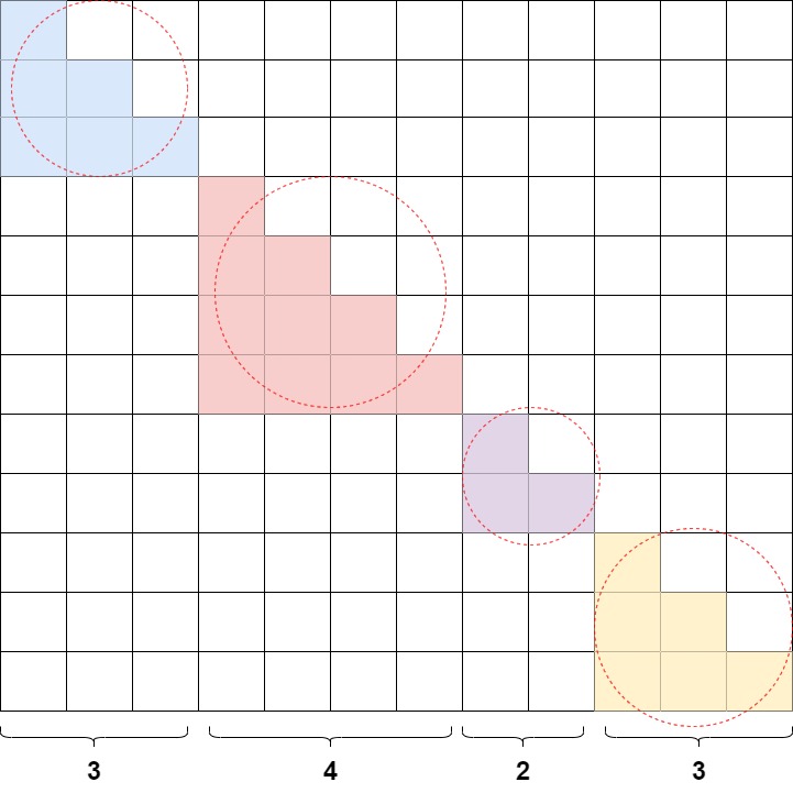
[0,3), [3,7), [7,9), and [9,12). A query may read earlier-or-equal keys only inside its own interval; every cross-interval cell is disallowed.Packing is semantically equivalent to separate examples only when every owned contract agrees:
| Contract | Separate examples | Equivalent packed representation |
|---|---|---|
| token content | each sequence has its own token rows | concatenation preserves every non-padding token in the intended order |
| visibility | causal support inside each example | block-diagonal causal support or equivalent varlen intervals |
| target pairs | next token belongs to the same declared stream | cross-segment prediction rows are ignored unless continuity is intentional |
| position geometry | each example starts from its declared position origin | position_ids reset or continue exactly as the model/data contract declares |
| objective weight | token/sequence weights are computed before padding | packed physical layout does not redefine numerator or denominator |
No single attention_mask proves all five. position_ids can delimit examples
for one kernel implementation while remaining only geometry for another.
Likewise, a varlen descriptor such as cu_seqlens can prevent cross-attention
but says nothing about the label on the last row of a segment.
A11 reuses the LongAlign figure below because it exposes the joint systems and objective problem: padding creates idle work, packing removes much of it, block-diagonal attention preserves sequence isolation, and loss weighting decides whether physical packs change sequence influence.
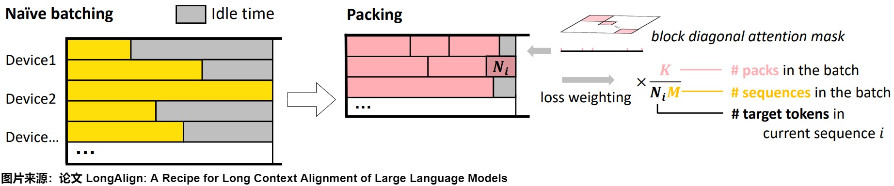
The figure is paper-specific. LongAlign’s weighting recipe is not a universal packing law; it is evidence that layout and objective weighting must be audited together. The separate Efficient Sequence Packing without Cross-contamination paper establishes packing as a bin-packing problem and tests mathematical equivalence for its model adaptations. Enhancing Training Efficiency Using Packing with Flash Attention compares several position/masking/packing combinations. Their names are not interchangeable implementation contracts.
Sorting, packing, and truncation alter the sample process
Length grouping can reduce padding and stragglers, but sorting also changes the order in which examples reach the optimizer. A deterministic packer can be described by one declared stage-order profile:
epoch seed
    -> global sample permutation
        -> optional length buckets with declared local/random order
            -> rank assignment
                -> deterministic packing plan
                    -> truncation/remainder policy
                        -> physical microbatches
The arrows above are not a commutation theorem. Changing the order of rank assignment and packing plan changes which
examples share a device and how many tokens each rank receives. With synchronous
data parallelism, every rank must execute compatible collective counts; a
packer that yields different numbers of microbatches can hang the job unless
the join/drop/pad policy is explicit.
Truncation needs a typed outcome:
truncate tail:
    keep prefix; record dropped target addresses

split with overlap:
    create new segment addresses; define duplicate-token loss ownership

defer whole sample:
    preserve example but carry packer remainder state

drop sample:
    change the training distribution and report it
Each outcome must retain the original sample/segment/token addresses, every
emitted occurrence-copy address, duplicate-copy group and unique downstream
owner, dropped/deferred intervals, stage-order version, and before/after packer
state. Naming truncate, split, defer, or drop without those receipts is
not enough to reconstruct target ownership or replay.
For response-only SFT, truncating before the first assistant target can produce a physically non-empty sequence with objective denominator zero. Filtering such rows, deferring them, or retaining them as context-only examples are different data policies.
Sampling probability and loss weight are separate levers
Suppose domain is sampled with probability , but the desired objective assigns domain mixture . For a sampled token from domain , an importance-weighted estimator can use
provided support and estimator assumptions hold. Oversampling a domain and also up-weighting its loss multiplies its influence. Conversely, changing only the sampler changes data order and frequency while leaving per-observation loss weight at one. Record both axes:
sample-selection distribution q
objective row/sequence weights w
Curricula add time dependence or , so their current phase and clock are checkpoint state. Empirical mixture choices remain source-reported; the equation does not claim importance weighting is always low variance or desirable.
Exact data resume is more than (epoch, seed)
For a map-style dataset, an epoch permutation might be a deterministic function only after the permutation algorithm, its byte-level inputs, tie behavior, and output order are versioned. Writing it as a mathematical set would lose order and repeated padded-tail occurrences, so a simple rank allocation is the ordered sequence
Real samplers may pad or drop the tail, form global batches before sharding, or balance token counts rather than sample counts. The exact rule is part of the manifest. PyTorch-style distributed samplers also require the epoch to be set consistently so a new permutation is selected rather than repeating one order.
Mid-epoch restart additionally needs the following state inventory:
| State | Why it matters |
|---|---|
| dataset/shard revision and global sample IDs | positional indexes are unsafe after corpus mutation |
| sampler epoch, seed, permutation algorithm, rank/world size, and cursor | reconstructs the next logical sample address |
| packer bins/remainders and truncation decisions | reconstructed samples can otherwise form different physical sequences |
| iterable-dataset source offsets | there may be no random-access permutation to replay |
| worker RNG derivation and persistent-worker state | corruption, augmentation, and local shuffle can differ |
| prefetch/in-flight queue | consumed versus merely produced samples must be distinguished |
| committed update/data transaction marker | prevents replaying or skipping work around asynchronous checkpoint capture |
This inventory is not itself replay proof. Exact replay additionally needs a defined state transition, a capture-consistency boundary, and a commit rule that distinguishes produced, issued, consumed, and durably committed work. Iterable-source offsets and worker fields are requirements until the selected input implementation can actually serialize and restore them.
Saving only dataloader loop index i is insufficient when workers have already
prefetched later examples. A practical exact-resume design either checkpoints
the complete producer state at a quiescent boundary or uses idempotent sample
addresses plus a committed cursor that lets queued work be regenerated safely.
0x05 Forward Pass: Known Targets Enter the Decoder All at Once
Now the training loop can call the model:
out = model.forward(
    batch.src,
    batch.tgt,
    batch.src_mask,
    batch.tgt_mask,
)
M3.1–M3.8 opened this model path. The dense full-vocabulary affine path below is one bounded M3.8 passport, not the only possible output interface. An adaptive, partitioned, sampled, or otherwise typed M3.8 head must expose its own admitted score and criterion socket before M3.9 can consume it. For the dense baseline, M3.9 now needs the training-side shape:
batch.src:       [B, S]
batch.tgt:       [B, T]
batch.src_mask:  [B, 1, S]
batch.tgt_mask:  [B, T, T]

out:             [B, T, d_model]
The decoder output has one row per target input position. It is not vocabulary logits yet:
out: [B, T, d_model]
This distinction is one of the most important implementation details in the source articles. In the Harvard implementation, EncoderDecoder.forward() does not call the generator. The generator is called later by SimpleLossCompute.
The training picture is therefore:
known source + known shifted target
    -> one masked forward pass
        -> one decoder hidden row per target position
The causal mask is why this is legal. Every row exists in the same tensor, but row t can only use target positions up to t.
At the objective level, nothing has stopped being autoregressive:
loss = - sum_{b,t : tgt_y[b,t] != PAD}
           log p_theta(tgt_y[b,t] | tgt[b,<=t], src_b)
The matrix form does not change the conditioning rule. It changes how many conditional distributions can be evaluated in one pass. For a single batch row:
| decoder input row sees | label row predicts |
|---|---|
<bos> | I |
<bos> I | ate |
<bos> I ate | an |
<bos> I ate an | apple |
<bos> I ate an apple | <eos> |
The model computes those rows together, but the target mask makes the row-wise conditioning match the autoregressive factorization.
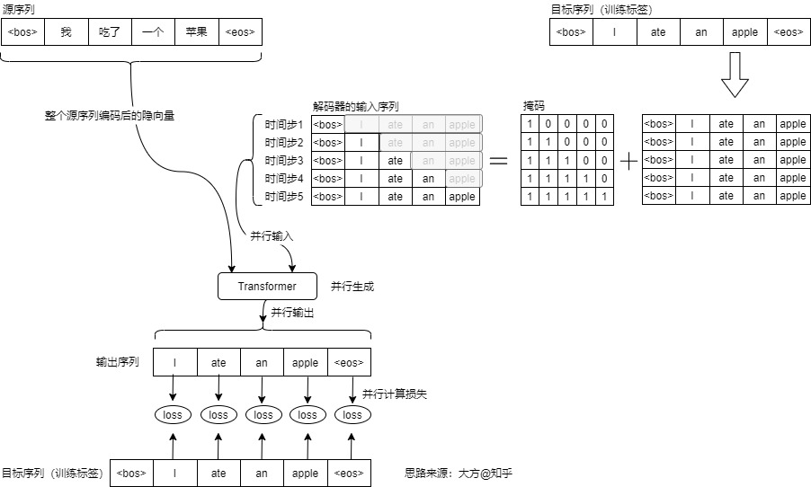
[BOS], [BOS,I], and so on are evaluated in one tensor; they predict I, ate, and later targets respectively, while each row's visibility ends at its own prefix.Read this figure as the local training object: shifted target input, mask, parallel decoder output, and one target-position loss per valid label.
0x06 SimpleLossCompute: Generator, Flatten, Criterion, Normalize
The next object is the loss-compute wrapper:
class SimpleLossCompute:
    def __init__(self, generator, criterion):
        self.generator = generator
        self.criterion = criterion

    def __call__(self, x, y, norm):
        x = self.generator(x)
        sloss = (
            self.criterion(
                x.contiguous().view(-1, x.size(-1)),
                y.contiguous().view(-1)
            )
            / norm
        )
        return sloss.data * norm, sloss
The inputs are:
x:
    out from model.forward(...)
    shape [B, T, d_model]

y:
    batch.tgt_y
    shape [B, T]

norm:
    batch.ntokens
    scalar count of non-pad labels
The first line applies the generator:
x = self.generator(x)
Shape:
[B, T, d_model] -> [B, T, V_tgt]
Depending on implementation, the generator may return raw logits or
log-probabilities. Those are different types, not merely prose conventions. A
criterion passport must state at least the ordered vocabulary identity, score
kind (logits or log_probabilities), dtype, admitted hard-class or frozen-
target type, ignore serialization, reduction (none at the local boundary),
and local VJP contract. In the Annotated Transformer style, the generator
applies log_softmax, and the criterion is built around KL divergence / label
smoothing. The generator and criterion passports must match exactly.
Then the batch and target-position dimensions are flattened:
x.contiguous().view(-1, x.size(-1))
y.contiguous().view(-1)
Shape:
generator output:
    [B, T, V_tgt] -> [B * T, V_tgt]

labels:
    [B, T] -> [B * T]
Conceptually, every admitted eligible prediction row becomes one local
vocabulary criterion row in this dense baseline. Padding, an unowned SFT
target, a broken continuation, or a non-owner duplicate may still occupy a
physical flattened row without being eligible for the objective.
Implementation-wise, contiguous() is not decorative. After slicing or
transposition, PyTorch tensors may not have a memory layout that view() can
flatten directly. The source code calls contiguous() before view() because
shape algebra is not the same thing as memory layout.
The criterion returns a summed loss, and the code normalizes it:
sloss = criterion(flat_x, flat_y) / norm
In this pinned baseline, using norm = batch.ntokens means:
normalize by real target labels,
not by rectangular padded positions.
That shorthand is valid only for the simple profile in which every non-PAD
target is query-valid, target-valid, policy-owned, a valid declared
continuation, an emitted copy, and the unique downstream-owner copy. General
packing, SFT, duplication, and weighted objectives use the six-term eligibility
join and the additive reduction below; they must not infer admission from
ntokens alone.
The return values have different purposes:
return sloss.data * norm, sloss
The first value is used for logging/token accounting. The second value, sloss, is still connected to the computation graph and is assigned to loss_node:
loss, loss_node = loss_compute(out, batch.tgt_y, batch.ntokens)
Only loss_node should receive:
loss_node.backward()
Calling .backward() on a detached logging value is a shape-invisible but fatal training bug.
0x07 LabelSmoothing: Target Distribution and PAD Exclusion
The criterion in the source training code is often:
criterion = LabelSmoothing(
    size=len(vocab_tgt),
    padding_idx=pad_idx,
    smoothing=0.1,
)
The class does two things at once:
1. build a smoothed target distribution
2. compute KLDivLoss against the generator output
The implementation begins with:
class LabelSmoothing(nn.Module):
    def __init__(self, size, padding_idx, smoothing=0.0):
        super(LabelSmoothing, self).__init__()
        self.criterion = nn.KLDivLoss(reduction="sum")
        self.padding_idx = padding_idx
        self.confidence = 1.0 - smoothing
        self.smoothing = smoothing
        self.size = size
        self.true_dist = None
After SimpleLossCompute flattens the tensors, LabelSmoothing.forward() receives:
x:       [B * T, V_tgt]    log-probabilities in this implementation
target:  [B * T]           target token IDs
It constructs:
true_dist: [B * T, V_tgt]
The core logic is:
assert x.size(1) == self.size
true_dist = x.data.clone()
true_dist.fill_(self.smoothing / (self.size - 2))
true_dist.scatter_(1, target.data.unsqueeze(1), self.confidence)
true_dist[:, self.padding_idx] = 0

mask = torch.nonzero(target.data == self.padding_idx)
if mask.dim() > 0:
    true_dist.index_fill_(0, mask.squeeze(), 0.0)

self.true_dist = true_dist
return self.criterion(x, true_dist.clone().detach())
For a non-pad target class y, vocabulary size V, pad index p, and smoothing
value epsilon, this exact recipe requires V >= 3, y != p, and
0 <= epsilon <= 1:
q_y = 1 - epsilon
q_p = 0
q_i = epsilon / (V - 2), for i not in {y, p}
For a row whose serialized target is padding:
stored ignore row = 0 for every vocabulary item i
That all-zero row is an ignore serialization, not a normalized target distribution . It is excluded before local-criterion admission and must not be passed downstream as though it were a probability distribution.
This is why the padding_idx handling appears twice:
zero the PAD column:
    do not assign smoothing mass to PAD

zero rows whose target is PAD:
    do not train on artificial padded labels
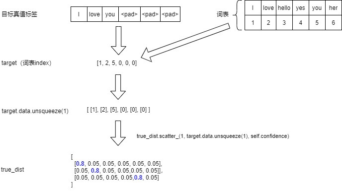
1-epsilon goes to gold, PAD gets zero, and epsilon is divided among the other V-2 classes. An all-zero serialized PAD row is ignored; it is not a target distribution.V >= 3, gold different from PAD, and epsilon in [0,1]. Then Q_gold=1-epsilon, Q_PAD=0, and every other class gets epsilon/(V-2).This section is easy to summarize incorrectly as “label smoothing makes one-hot labels softer.” That is true but too incomplete for implementation. In this code, label smoothing is also where vocabulary size, pad index, flattened target rows, and the loss function meet.
Cross entropy from the autoregressive likelihood
For one valid target row with class and logits ,
Substitute softmax:
The stable implementation subtracts the row maximum :
Differentiation yields
This expression structurally couples the loss to the vocabulary row, but it
does not guarantee a nonzero value in every coordinate: a coordinate can be
exactly zero when , and the sole coordinate of a degenerate
V=1 softmax is zero. M3.8 owns the head-level interpretation; M3.9 owns which
admitted training rows and coefficients form the scalar reduced across devices.
Label smoothing as a mixture target
A common conceptual target is
where distributes mass over allowed non-target classes. Cross entropy becomes
For a complete, normalized, parameter-independent target distribution ,
minimizing smoothed cross entropy is equivalent to minimizing KL divergence
from the fixed target distribution up to the constant . Under those same
conditions their raw-logit VJPs agree, although their scalar values differ.
This explains why the Harvard implementation can use KLDivLoss on
log-probabilities.
The exact convention differs:
Harvard shown above:
    target class gets 1-epsilon
    PAD gets zero
    epsilon spread over V-2 remaining rows

some framework cross-entropy implementations:
    mix with uniform mass over all V classes,
    so the target also receives epsilon/V
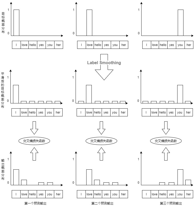
Both can be called label smoothing while producing different targets. Reproducing a run requires the exact formula, ignore-index behavior, reduction, and denominator.
The source-series figure below contrasts one-hot targets, smoothed targets, and model probability rows over several positions. It is an intuition diagram: the exact mass allocation still comes from the declared formula, not from the bar heights.
The general weighted row objective
criterion(...) / ntokens is one special case of a more general reduction.
Index every materialized prediction row by . Let:
Q_r(v): frozen admitted target distribution for vocabulary item v
p_r(v): model probability for vocabulary item v
e_r:    six-term eligible-row predicate defined above
a_r:    non-negative numerator coefficient
b_r:    non-negative denominator coefficient
The unreduced cross entropy of row is
Define the objective numerator and denominator separately:
Then
Both coefficient arrays and are fixed data, or explicitly stop-gradient, for the VJP shown below. Keeping and separate prevents one normalized-weight profile from being mistaken for every weighted estimator. This form identifies common policy choices:
| Policy | a_r | b_r | Denominator identity |
|---|---|---|---|
| ordinary token mean | e_r | e_r | eligible target-copy rows |
| response-only SFT | e_r with assistant target policy | same as a_r | eligible assistant-owned targets |
| per-sequence mean | e_r / N_s for semantic sequence s | e_r / N_s | number of non-empty semantic sequence identities, not physical packs |
| self-normalized domain/importance weighting | e_r w_r | e_r w_r | selected weight mass |
| count-normalized weighted objective | e_r w_r | e_r | eligible-row count; a distinct objective, not an error by definition |
| fixed microbatch mean | e_r / N_m inside non-empty microbatch m | e_r / N_m | number of non-empty microbatches; differs from token mean unless conditions align |
For complete normalized frozen , the logit gradient follows directly. Because ,
Rows with e_r = 0 have a_r=b_r=0 and contribute no local objective. Whether
a larger weight changes the numerator, denominator, or both is part of the
declared objective. Multiplying only the numerator is not universally wrong; it
defines the distinct count-normalized weighted profile above. What is wrong is
claiming one profile while implementing another.
The zero-denominator case must be a typed objective result. A microbatch can
contain no eligible rows after truncation or response-only masking, or it can
contain eligible rows whose declared denominator coefficients are all zero.
These causes are different even though both project to GLOBAL_ZERO_MASS after
the relevant accumulation/distributed scope. There is then no scalar objective
and no objective cotangent. This layer does not decide whether later update
policy replays, skips, or otherwise disposes of the window:
row_loss = admitted_local_criterion(scores, targets, reduction="none")
eligible = (query_valid & target_valid & policy_owner
            & continuation_valid & emitted_copy & unique_copy_owner)
numerator_coeff = eligible * row_numerator_coeff
denominator_coeff = eligible * row_denominator_coeff

numerator = (row_loss * numerator_coeff).sum(dtype=torch.float32)
denominator = denominator_coeff.sum(dtype=torch.float64)

if denominator == 0:
    cause = ("EMPTY_ELIGIBLE_SET" if not eligible.any()
             else "NONEMPTY_ZERO_WEIGHT_MASS")
    return NoObjective(state="GLOBAL_ZERO_MASS", cause=cause)
else:
    return ScalarObjective(value=numerator / denominator)
In an accumulation or distributed window, a locally empty microbatch need not force a globally empty objective. The global objective state is formed only after the declared numerator and denominator scope is complete. Even then, objective construction exports a scalar/cotangent or a typed no-objective state; later update policy owns the action.
Label-smoothing conventions are different objectives
For vocabulary size , gold class , PAD class , and smoothing , the Harvard source path uses:
The row sums to one because
Another common implementation mixes a one-hot target with the uniform distribution over all classes:
Then the gold class receives and PAD receives
unless ignore_index removes the whole row. A third convention
mixes over all non-PAD classes, giving the target some of the uniform mass but
none to PAD. These variants have different gradients even when all are called
label_smoothing=0.1.
Also separate the optimized quantity from the reported one:
For complete normalized frozen , minimizing smoothed cross entropy and KL divergence has the same parameter minimizer and raw-logit VJP, but their scalar values differ by . Those conclusions do not automatically extend to an incomplete, unnormalized, or parameter-dependent target. A training log that changes from CE to KL without recording the convention has a discontinuity even when the admitted gradients agree.
Token mean, sequence mean, and microbatch mean are different objectives
Token-normalized loss is
Sequence-normalized loss first averages each sequence:
The second gives a short sequence and long sequence equal total weight; the first gives each valid token equal weight. Equal averaging of microbatch means adds a third weighting. Dataset mixture weights, curriculum sampling, and packed sequence lengths interact with this choice even if the same tokens are observed.
For two sequences with token-loss sums and counts ,
while
If , these expressions generally differ. Packing does not decide which is correct; the experiment contract does. LongAlign, for example, explicitly studies packing together with loss weighting because physically placing several sequences in one pack must not accidentally redefine their relative objective weight.
Perplexity is an aggregate of unsmoothed negative log-likelihood
For a held-out token set, perplexity requires a separate authenticated gold-NLL evaluation socket: the exact checkpoint/artifact and head passport, ordered vocabulary, gold hard-class targets, eligibility policy, natural-log criterion, dataset/split identity, and global aggregation manifest must all be frozen. Given accepted total gold NLL and accepted eligible-token count ,
This uses natural logarithms. With base-2 logarithms, the corresponding exponential base is 2. More importantly, the conventional language-model perplexity is computed from the gold one-hot NLL, even if training used label smoothing. Exponentiating a smoothed CE/KL training scalar produces a different quantity and should not be reported as directly comparable perplexity.
Perplexity aggregation must preserve the same numerator/denominator order:
global_nll = completed_all_reduce_sum(local_gold_nll_sum)
global_tokens = completed_all_reduce_sum(local_eligible_gold_tokens)
mean_nll = global_nll / global_tokens if global_tokens > 0 else NA
ppl = exp(mean_nll) if isfinite(mean_nll) and exp_is_finite(mean_nll) else NA
Averaging per-sequence, per-batch, or per-rank perplexities is invalid because
the exponential is nonlinear. Report zero-token evaluation shards separately;
evaluate the final ratio only when the global denominator is positive; and
publish PPL only when both the mean NLL and its exponentiation are finite.
Otherwise the result is explicitly N/A, together with its cause—not a silently
clamped or overflowed metric.
0x08 Backward, Accumulation, Optimizer, Scheduler
After the scalar loss node is created, the training loop turns it into gradients and parameter updates:
At the formal boundary there are two mutually exclusive seed routes: one
declared global scalar objective root, or one explicitly supplied cotangent for
typed score rows. A transaction uses exactly one route. The objective has
already applied its one declared denominator, so no child denominator,
ntokens, rank count, or accumulation-count division may be applied again.
The complete window is bound to one parameter revision, graph/linearization
revision, alias map, parameter-presence roster, objective revision, and set of
logical gradient owners. A detached logging scalar is neither seed route.
if mode == "train" or mode == "train+log":
    loss_node.backward()
    train_state.step += 1
    train_state.samples += batch.src.shape[0]
    train_state.tokens += batch.ntokens

    if i % accum_iter == 0:
        optimizer.step()
        optimizer.zero_grad(set_to_none=True)
        n_accum += 1
        train_state.accum_step += 1

    scheduler.step()
The basic path is:
loss_node.backward():
    compute gradients through generator, decoder, encoder, embeddings, etc.

optimizer.step():
    update parameters using accumulated gradients

optimizer.zero_grad(set_to_none=True):
    clear gradients for the next accumulation window

scheduler.step():
    update learning-rate state
The source code uses gradient accumulation:
if i % accum_iter == 0:
    optimizer.step()
    optimizer.zero_grad(set_to_none=True)
Backward happens every training batch. Optimizer step happens only on the accumulation cadence. The source also calls:
scheduler.step()
every training batch after the accumulation block. If this cadence is changed, it should be changed intentionally. It is easy to claim “scheduler steps when optimizer steps,” but that is not what this source loop shows.
The source includes a commented line:
# loss_node = loss_node / accum_iter
This is worth noticing. In gradient accumulation, one must decide whether to scale each microbatch loss by accum_iter, change the learning rate, or accept a different effective gradient scale. The source line is commented, so M3.9 should not pretend accumulation is automatically scale-correct without explanation. The safe statement is: accumulation changes update cadence, and loss scaling must be handled deliberately.
Quantitative accumulation audit
There are two separate invariants: when an update occurs and what objective its accumulated gradient represents.
The displayed source loop enumerates from zero. With accum_iter=4 and eight
microbatches indexed 0..7, its condition i % accum_iter == 0 steps at:
i = 0: update after one microbatch
i = 4: update after microbatches 1,2,3,4
i = 5,6,7: gradients remain unstepped when the loop exits
That is not four-plus-four accumulation. A full-window condition is normally
based on (i + 1) % accum_iter == 0, and the final partial window must be
flushed explicitly. This is a source-level off-by-one and remainder hazard, not
a property of gradient accumulation itself.
Loss scaling has a second trap. Let microbatch contain real target tokens and let be its token-mean loss. The exact token-normalized objective for an accumulation window is:
Simply dividing every by the number of microbatches computes an equal
microbatch average. It equals the token average only when all are equal.
A reference implementation can backpropagate each unnormalized token sum
loss_node * batch.ntokens, accumulate window_tokens, divide accumulated
gradients by that token count, and then update:
pending = 0
window_tokens = 0
optimizer.zero_grad(set_to_none=True)

for i, batch in enumerate(data_iter):
    out = model.forward(
        batch.src, batch.tgt, batch.src_mask, batch.tgt_mask
    )
    loss, loss_node = loss_compute(out, batch.tgt_y, batch.ntokens)
    (loss_node * batch.ntokens).backward()
    pending += 1
    window_tokens += int(batch.ntokens)

    if pending == accum_iter:
        for p in model.parameters():
            if p.grad is not None:
                p.grad.div_(window_tokens)
        optimizer.step()
        optimizer.zero_grad(set_to_none=True)
        scheduler.step()
        pending = 0
        window_tokens = 0

# Repeat the same divide/step/zero sequence when pending > 0.
That snippet is single-process. Distributed data parallelism adds a specific
normalization factor, not just a vague reduction step. Let rank r accumulate
an unnormalized token-sum gradient g_r, let R be the world size, and let:
For the bounded profile used in this derivation—PyTorch DDP’s default reducer, fixed initial world size , no custom communication hook, no join-mode divisor change, and a common parameter-use/bucket contract—the synchronized gradient is world-size averaged, so each replica holds:
The desired global token-mean gradient is therefore:
Each rank must all-reduce the token count and scale the synchronized gradient by
world_size / global_tokens. Dividing by each rank’s local token count gives
different objectives when padding or sequence lengths differ across ranks.
Communication cadence matters too. Under DDP, the first accum_iter-1
forward/backward calls can run inside model.no_sync(); the final call exits
that context and synchronizes the accumulated gradients. The forward pass must
also be inside no_sync(), as required by the PyTorch contract. Synchronizing
every microbatch is mathematically usable but pays an all-reduce every time and
defeats the communication-saving purpose of accumulation.
Mixed precision fixes the remaining order. Keep one loss scale throughout the
effective batch, accumulate scaled gradients, call scaler.unscale_(optimizer)
once after the final backward, apply the global token-normalization factor, then
clip, step, and update the scaler. Unscaling or changing the scale before the
window is complete mixes incompatible gradient scales. If the scheduler is
optimizer-step based, stepping it once per microbatch advances the learning-rate
schedule accum_iter times faster than the parameter updates.
When accumulation is exactly a large-batch gradient
The source-series diagram below compares several small batches accumulated at fixed weights with one larger batch. Its approximation note concerns taking an optimizer update between small batches. Exact gradient accumulation does not do that: all microbatches in the window differentiate the same parameter state.
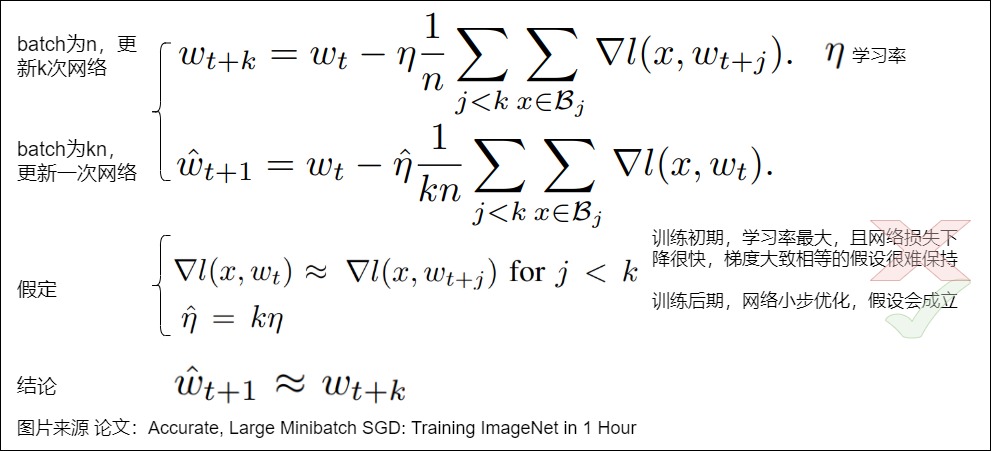
Let microbatch have weighted loss numerator and denominator . The effective-window objective is
Because differentiation is linear and every microbatch uses the same ,
There are two exact implementation forms:
form A: accumulate unnormalized numerator gradients
    backward(S_m) for every m
    divide parameter gradients by D_W once at update boundary

form B: pre-scale each numerator when D_W is known
    backward(S_m / D_W) for every m
Backpropagating each microbatch mean and dividing by instead computes
which equals the window token mean only under special cases such as equal denominators. Dividing by the configured accumulation count also mishandles a final partial window unless its actual count and token denominator happen to match the full window.
The word exact is bounded by the execution contract:
| Condition | Required for what kind of equivalence? |
|---|---|
| no optimizer step inside the window | same parameter point for every microbatch gradient |
| same examples, row weights, masks, and total denominator | same mathematical objective |
| gradient summation in exact arithmetic | algebraic gradient equivalence |
| same floating-point reduction order | bitwise gradient equivalence, usually not guaranteed |
| same stochastic masks per logical example | same stochastic realization rather than only same distribution |
| stateful layers updated equivalently | same non-parameter state; dropout has no running state, BatchNorm does |
Even when the algebra matches, separate microbatch kernels can sum in a different order from one large-batch kernel. Floating-point results can differ slightly. That does not make the objectives different, but it limits bitwise claims.
Nonlinear operations belong after the complete gradient
Global-norm clipping is nonlinear. For clipping operator
in general
Here the clip passport must freeze , the exact non-negative stabilizer
, comparison boundary (< or <= at the threshold), norm dtype,
parameter/alias/shard owner map, handling of zero, absent, sparse, and
non-finite gradients, and the collective completion rule. The norm is over each
logical gradient exactly once; counting aliases or replicated copies changes
the operator.
Clipping each microbatch gradient and then summing does not simulate clipping
the effective-batch gradient. The same applies to Adam moment updates: calling
optimizer.step() after every microbatch produces state transitions and
evaluates later gradients at changed parameters. It is not gradient
accumulation.
The transaction boundary is therefore, for a declared physical profile:
for each microbatch in window:
    forward at the same parameter version
    form weighted numerator
    backward numerator
    retain accumulated gradients and denominator

once at window close or final remainder:
    complete every declared gradient collective and its completion token
    obtain the global denominator and unique logical-owner roster
    unscale each active optimizer exactly once if FP16 scaling is active
    apply the one declared global normalization under the reducer convention
    evaluate the closed finite predicate over all declared owners/buffers
    compute one binary32 norm over unique logical parameters and clip once
    optimizer step once if finite
    zero gradients
    scaler update
    scheduler/counters advance only under declared success policy
An update attempt and a committed update are different events. If a finite check rejects the gradient, the declared skip-all policy keeps model parameters, optimizer moments, and an update-based scheduler at the old committed version. That atomic skip across every optimizer is a policy this article selects; it is not a universal promise of each framework scaler. The data cursor and attempted-token counter may still advance; that policy must be manifested because replaying or dropping the rejected window changes the run. Logical all-old/all-new selection, physical writes, scaler state, disposition logging, and durable checkpoint publication are separate transitions. A finite flag alone does not make them fault-atomic across rank or process failure.
A denominator-safe local accumulation skeleton
optimizer.zero_grad(set_to_none=True)
pending_microbatches = 0
window_denominator = torch.zeros((), dtype=torch.float64, device=device)
window_has_objective = False

for is_last, batch in with_last(data_iter):
    logits = model(batch)
    row_loss = criterion(logits, batch.labels, reduction="none")
    weights = batch.loss_owner * batch.row_weight
    numerator = (row_loss * weights).sum(dtype=torch.float32)
    denominator = weights.sum(dtype=torch.float64)

    if denominator > 0:
        scaled_backward(numerator)  # unnormalized S_m
        window_has_objective = True
    window_denominator += denominator
    pending_microbatches += 1

    close = pending_microbatches == accum_iter or is_last
    if close:
        objective_state = classify_global_objective(window_has_objective,
                                                    window_denominator)
        if objective_state == "SCALAR_OBJECTIVE":
            unscale_if_needed_exactly_once(optimizer)
            divide_gradients_(model.parameters(), window_denominator)
            finite = closed_owner_roster_is_finite()
            if finite:
                clip_grad_norm_(model.parameters(), max_norm)
                optimizer.step()
                scheduler.step()  # successful-update schedule
            update_scaler_from_attempt_result(finite)
        else:
            record_no_objective(objective_state)
            # No backward/update attempt occurred: do not advance scaler growth.
        optimizer.zero_grad(set_to_none=True)
        verify_present_gradient_buffers_cleared_and_absent_ones_still_absent()
        pending_microbatches = 0
        window_has_objective = False
        window_denominator.zero_()
This is a single-process semantic skeleton, not framework-ready code. Its
zero_grad(set_to_none=True) call is an intent until the implementation records
before/after receipts for every present physical gradient buffer while keeping
absent, frozen, and no-objective states distinct. The distributed and numerical
sections below add DDP’s averaged all-reduce factor, no_sync() placement,
sharded norms, fixed-window loss scaling, globally agreed finite checks, and
recomputed RNG state.
The optimizer and scheduler are constructed like this:
optimizer = torch.optim.Adam(
    model.parameters(),
    lr=config["base_lr"],
    betas=(0.9, 0.98),
    eps=1e-9,
)

lr_scheduler = LambdaLR(
    optimizer=optimizer,
    lr_lambda=lambda step: rate(
        step, d_model, factor=1, warmup=config["warmup"]
    ),
)
The rate() function implements the Noam-style schedule:
def rate(step, model_size, factor, warmup):
    if step == 0:
        step = 1
    return factor * (
        model_size ** (-0.5) * min(step ** (-0.5), step * warmup ** (-1.5))
    )
Equation:
lrate = factor * d_model^(-0.5)
        * min(step^(-0.5), step * warmup^(-1.5))
The first phase warms up. The later phase decays.
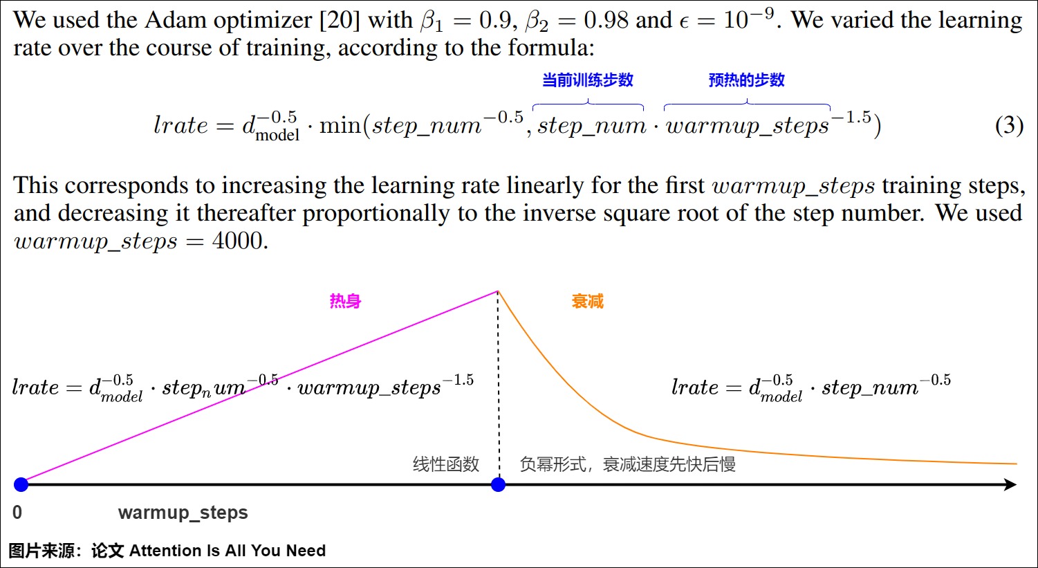
w and then decays with inverse square root. The scheduler passport must state which clock is used and distinguish the value visible before an attempt, the value used by a committed update, and the next value.eta(t)=c*d_model^(-1/2)*min(t^(-1/2), t*w^(-3/2)); the branches meet at t=w. Under a successful-update clock, rejected or no-objective windows do not advance t.Adam state and bias correction
For gradient , Adam maintains first and second moments:
Zero initialization biases both estimates toward zero, so Adam uses
and updates
The step counter is optimizer state. Restoring weights without moments and step creates a different training trajectory even if the next batch and learning-rate value look correct.
AdamW decouples weight decay:
Applying L2 regularization inside is not generally equivalent under Adam’s adaptive denominator. Bias, norm, and embedding parameters are often assigned different decay policies; that parameter-group map is checkpointed training configuration.
Optimizer families change state, scale, and migration
The optimizer name is not a minor implementation detail after the objective is fixed. It determines persistent state, the nonlinear transformation applied to the gradient, and what must be migrated with a checkpoint.
Plain SGD applies
Momentum adds a velocity state:
Adam keeps parameter-shaped first and second moments. Adafactor instead factorizes the second-moment estimate of a matrix into row and column statistics. Its auxiliary second-moment storage can scale like rather than for that matrix. The paper also introduces update clipping, a changing second-moment decay, and parameter-scale-relative steps; selecting only “factored state” is not the complete paper contract.
LAMB begins from an Adam-like direction and applies a layer/tensor trust ratio, schematically:
The exact clipping, decay, zero-norm, and bias-correction rules belong to the chosen implementation. LAMB’s source-reported large-batch results do not make it a universal replacement for AdamW.
| Family | Persistent auxiliary state per parameter | Distinctive transition | Migration consequence |
|---|---|---|---|
| SGD | none | raw gradient | easiest warm start; still preserve schedule/update counters |
| momentum SGD | one velocity | exponentially averaged direction | dropping velocity changes next update |
| Adam/AdamW | first moment, second moment, step | coordinate-wise adaptive denominator; AdamW decouples decay | moments, per-parameter step, groups, and decay policy are required |
| Adafactor | factored or full second moment; optional first moment by configuration | factored adaptive scale and update clipping | state shape depends on parameter rank and implementation options |
| LAMB | Adam-like moments and trust-ratio state/convention | tensor/layer norm ratio scales adaptive direction | parameter grouping and norm boundaries are part of the contract |
The storage table is conceptual. Fused, sharded, quantized, or master-weight implementations change physical bytes without changing the logical state that a resume must reconstruct.
For every logical parameter and optimizer field, PRESENT_NONZERO,
PRESENT_EXACT_ZERO, ABSENT, FROZEN, and NOT_APPLICABLE are distinct
states. A zero moment is data; a missing moment may mean uninitialized,
unsupported, or corrupt; a frozen parameter owns no update; and a per-parameter
step can differ from a group/global clock in some algorithms. Save/load and
migration rules must preserve those distinctions rather than fill missing state
from shape alone.
Parameter groups are named update policy
A weight-decay rule is applied to parameters, not to textual substrings. A robust builder resolves aliases, assigns each unique parameter exactly once, and hashes the result:
decay = []
no_decay = []
seen_parameter_ids = set()

for module_path, module in model.named_modules():
    for local_name, parameter in module.named_parameters(recurse=False):
        address = f"{module_path}.{local_name}".lstrip(".")
        parameter_id, aliases = parameter_registry.resolve(
            model_schema_id=model_schema_id,
            address=address,
            parameter=parameter,
        )
        if parameter_id in seen_parameter_ids:
            continue  # tied embedding/head or another alias
        seen_parameter_ids.add(parameter_id)

        if is_declared_norm_or_bias(module, local_name):
            no_decay.append((parameter_id, aliases, parameter))
        else:
            decay.append((parameter_id, aliases, parameter))

assert_unique_and_complete(decay, no_decay, model)
parameter_group_sha256 = hash_addresses_and_hyperparameters(
    decay=decay,
    no_decay=no_decay,
)
data_ptr() may help inspect aliasing inside one live process, but allocation
addresses change across save/load and are not stable parameter or optimizer
state identities. The registry above is a required logical mapping: canonical
fully qualified names, explicit alias groups, model-schema revision, shapes,
dtypes, presence state, and unique ownership. Using parameter.ndim == 1 as a
no-decay shortcut is a policy, not a theorem;
it can classify embeddings, gates, or unusual parameters incorrectly. Name
matching alone is also fragile under refactors. The manifest should record
resolved parameter IDs and aliases, group order, decay kind (decoupled or
coupled), exact hyperparameters/flags, state schema, and an authenticated
payload digest. Resolving or changing any of those fields creates a new update
identity and requires explicit optimizer/progress migration before state is
attached.
A learning-rate schedule needs a clock
The word step can mean at least four counters:
microbatch step:
    every attempted forward/backward transaction

successful update step u:
    every optimizer transition actually committed

global supervised-token count tau:
    total valid objective denominator committed across ranks

sample/sequence count:
    examples committed, sensitive to packing and variable length
Noam in the Transformer paper is expressed using an update-like step. A cosine decay over successful updates can be written
A token-clock schedule instead uses , for example linear warmup to followed by cosine decay to token budget :
Token clocks make a schedule less sensitive to changed microbatch and packing
shapes, but only if tau is the globally reduced committed supervised
denominator. Counting padded or attempted tokens produces another clock.
Cosine warm restarts, polynomial decay, constant-with-warmup, inverse-square- root, and warmup-stable-decay schedules all define different curves and state. Their reproducibility tuple is:
family + all hyperparameters + clock type + current clock value
+ update-skip policy + endpoint behavior + restart/cycle state
+ learning rate visible before the attempt
+ learning rate actually used by every committed parameter group
+ next learning rate after the declared clock transition
+ separate no-objective, rejected-attempt, and committed-update dispositions
These values are not interchangeable. A scheduler can expose a “current” value while the optimizer used the prior value, and a rejected or no-objective window may leave both the update clock and next learning rate unchanged under the declared successful-update policy.
Changing effective batch size and scaling the learning rate is an empirical optimization choice, not part of gradient-accumulation equivalence. Linear scaling and warmup have source-reported successes in large-batch regimes, but the valid scaling range depends on optimizer, model, data, and gradient noise.
Deriving the Noam peak
The schedule is
with warmup . The branches meet when
Therefore the learning rate rises linearly until the warmup step and peaks at
then decays as . The scheduler’s definition of t must match actual optimizer updates, not merely dataloader iterations, when gradient accumulation is active.
Gradient clipping order under mixed precision
For the declared clip passport, global norm clipping computes
and scales by
Under loss scaling , backward produces . Clipping before unscale compares with threshold and over-clips by the scale factor. The scale is bound to the complete accumulation window and active optimizer, and the one-time-unscale receipt must be present before the clip-ready state. The order is:
accumulate scaled backward passes
    -> unscale optimizer gradients once
    -> apply global token/world-size normalization
    -> check finite gradients
    -> clip unscaled global norm
    -> optimizer step
    -> update loss scaler
    -> scheduler step if update succeeded
If overflow causes the scaler to skip an optimizer update, an update-count-based scheduler should not advance as though parameters changed.
Precision is a graph of states, not one dtype
The phrase “train in BF16” is incomplete. A compact introduction starts with four numerical roles:
| Role | Example policy | Why it is separate |
|---|---|---|
| parameter storage | BF16 model weights or FP32 weights | determines persistent model representation |
| operator compute | autocast selects BF16/FP16 GEMMs and safer reduction paths | different operators have different range and accuracy needs |
| accumulation/reduction | FP32 dot-product accumulation, norm/loss sums, and collective buffers | long reductions amplify rounding and overflow risk |
| optimizer state | FP32 master parameters and FP32 moments in a common mixed-precision recipe | small updates and moment history can be lost in narrow formats |
The common binary formats illuminate the tradeoff:
| Format | Exponent bits | Fraction bits | Approximate largest finite value | Training consequence |
|---|---|---|---|---|
| FP32 | 8 | 23 | broad range and finer precision, higher traffic/storage | |
| BF16 | 8 | 7 | FP32-like range with coarse significand | |
| FP16 | 5 | 10 | finer significand than BF16 but much narrower range | |
| TF32 matmul mode | 8 | about 10 effective input fraction bits | FP32-like range | NVIDIA matmul execution policy, not a checkpoint storage dtype |
Subnormal handling and flush-to-zero behavior depend on the device and kernel. Those details are runtime state, not facts implied by the file extension. Likewise, autocast is an operator policy: a matrix multiply, softmax, norm, loss reduction, and optimizer update need not execute in the same dtype. The exact allowlist and promotion behavior are framework-, device-, and version-specific.
A reproducible precision passport must go further. For every logical parameter, master copy, activation family, score/logit row, local loss, numerator, denominator, gradient buffer, collective buffer, norm accumulator, finite predicate, optimizer state, and checkpoint field, it records storage, input, compute, accumulation, reduction, and output dtypes where applicable. It also binds device/backend, autocast implementation and version, enabled regions, explicit casts, rounding and subnormal policy, scaler identity/configuration, and the owner/completion receipt for each conversion. This passport selects a logical numerical branch; later physical realization and durable publication are separate evidence layers.
Why loss scaling works, and where it stops working
Let be the loss scale. Backward on
produces
If the scaled gradient remains finite, dividing by recovers in exact arithmetic. The practical benefit is that small intermediate gradients are shifted into FP16’s representable range before they underflow. Scaling cannot repair a forward activation that already overflowed, and a scale that is too large can overflow the backward pass.
All microbatches in one accumulation window must use the same :
If the scale changes from to without first separating or unscaling the stored gradients, the buffer contains and no single division recovers .
A dynamic scaler is a feedback controller, not part of the mathematical objective:
overflow on attempted update:
    skip every parameter/optimizer/scheduler update
    next_scale = current_scale * backoff_factor

growth_interval successful updates:
    next_scale = current_scale * growth_factor

otherwise:
    next_scale = current_scale
In the pinned PyTorch GradScaler state dictionary, the five scalar fields are
scale, growth_factor, backoff_factor, growth_interval, and
_growth_tracker. An article-level rejected/skipped-attempt counter can be
useful audit state, but it is not one of those five framework fields and
must be stored in a separate disposition ledger. A GLOBAL_ZERO_MASS
no-objective window made no scaler-backed update attempt, so it must not be
reported to the scaler as a successful finite attempt merely to advance the
growth tracker.
Distributed finite checking is one decision
In a replicated or sharded run, every rank and pipeline stage must agree on whether the logical update commits:
where means every declared gradient and required optimizer-facing buffer in rank ‘s closed participant roster passes the declared finite predicate. The roster binds ranks, pipeline stages, unique logical storage/alias owners, buffer presence states, predicate dtype, process group, collective sequence, and completion token. If one tensor-parallel shard overflows while another stage steps, the checkpoint no longer represents one parameter version.
An implementation may obtain this agreement implicitly when infinities propagate through an authenticated replicated-gradient profile, or explicitly by reducing a finite flag and waiting for completion. Neither route is universal across sharded buffers or custom communication hooks. The declared semantic contract is:
close accumulation window
-> finish required gradient collectives
-> unscale exactly once
-> apply declared global loss normalization
-> reduce finite flags across every update owner
-> if finite: global logical clip -> optimizer step
-> if not finite: no parameter or optimizer transition
-> update scaler on every owner from the same result
-> advance update-based scheduler only after a committed step
Loss normalization and unscaling commute in exact arithmetic because both are linear scalar divisions. Neither commutes with clipping. Framework APIs can also track whether an optimizer has already been unscaled, so production code should follow the runtime’s required call order rather than manually reaching into scaler internals.
Activation checkpointing replays a stochastic program
Activation checkpointing saves selected boundary tensors and recomputes an interior forward region during backward. If an ordinary block stores activation state and costs forward work , checkpointing approximately trades some of that saved for another execution of selected forward operators. The exact memory and compute change depends on the partition; it is not a universal “half memory, twice compute” rule.
For a stochastic region,
the random state is an input to the realized forward graph. Backward must recompute with the same dropout mask, not . Otherwise it differentiates a different sampled function.
def checkpointed_region(x):
    # The checkpoint runtime preserves or reconstructs the RNG state that
    # existed when this region ran in the original forward.
    return dropout(ffn(x), p=0.1, training=True)

y = checkpoint(checkpointed_region, x, preserve_rng_state=True)
PyTorch exposes reentrant and non-reentrant checkpoint mechanisms with
different recording and recomputation behavior; current documentation
recommends passing use_reentrant explicitly. The article’s invariant is
implementation-independent: recomputed values, side effects, collectives, and
random draws must satisfy the selected checkpoint contract.
RNG ownership and topology
One integer seed is not complete stochastic state. The immutable manifest and mutable progress payload must name and address every stochastic stream. A large training run can have separate streams for:
dataset permutation and worker-local augmentation
token corruption or span masking
dropout in replicated layers
tensor-parallel-consistent dropout
sequence-parallel token-local dropout
pipeline-stage stochastic operators
sampling used by alternative training procedures
Saving only the initial seed does not reveal each stream’s current counter. Exact resume saves generator states or reproducible counter addresses together with algorithm/version, device, topology/replication rule, and the next semantic event address. A topology-stable counter design can derive a random block from semantic keys such as:
(run_seed, global_sample_id, layer_id, operator_id, logical_token_address)
rather than from “whatever rank happened to execute next.” That design is not free: replicated operators that require identical masks must share addresses, while token-sharded operators require disjoint addresses. Changing tensor, sequence, or pipeline topology therefore needs an explicit RNG migration policy.
For a checkpointed region, preserved RNG is necessary but not sufficient. A recompute receipt also binds the region/graph revision, checkpoint variant, device migration, autocast context, parameter/buffer versions, input values, side effects and collective order, output-value comparator, and early-stop policy. Deterministic replay also has a boundary. The same masks and batches do not guarantee bitwise results when kernels, collective trees, compiler schedules, or floating-point reduction order change. The release contract should say whether it promises exact replay on a pinned stack, numerical closeness, or only statistical equivalence.

The precision transaction and recomputation transaction meet at backward, but they own different state: the scaler controls gradient representation; the checkpoint runtime controls which forward values and RNG states are replayed.
Again, this is not a separate optimizer article. It belongs here because loss_node.backward() is not the end of training. The scalar loss only matters because it produces gradients that the optimizer and scheduler use to change model parameters.
0x09 Train/Eval Mode and Dropout
The source training worker switches modes explicitly:
model.train()
run_epoch(..., mode="train+log", optimizer=optimizer, scheduler=lr_scheduler)

model.eval()
run_epoch(
    ...,
    optimizer=DummyOptimizer(),
    scheduler=DummyScheduler(),
    mode="eval",
)
This is not only a bookkeeping convention. It changes the forward pass because dropout behaves differently in training and evaluation.
The handwritten training article shows dropout at several Transformer locations:
after token embedding + positional encoding
after attention softmax, on attention weights
inside the feed-forward network
inside the sublayer/residual wrapper
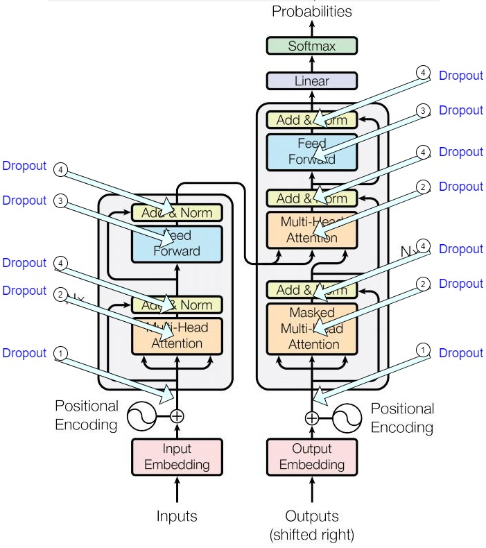
In code:
class PositionalEncoding(nn.Module):
    def forward(self, x):
        x = x + self.pe[:, : x.size(1)].requires_grad_(False)
        return self.dropout(x)
def attention(query, key, value, mask=None, dropout=None):
    scores = torch.matmul(query, key.transpose(-2, -1)) / math.sqrt(d_k)
    if mask is not None:
        scores = scores.masked_fill(mask == 0, -1e9)
    p_attn = scores.softmax(dim=-1)
    if dropout is not None:
        p_attn = dropout(p_attn)
    return torch.matmul(p_attn, value), p_attn
class PositionwiseFeedForward(nn.Module):
    def forward(self, x):
        return self.w_2(self.dropout(self.w_1(x).relu()))
class SublayerConnection(nn.Module):
    def forward(self, x, sublayer):
        return x + self.dropout(sublayer(self.norm(x)))
Module mode and autograd recording are separate controls. model.eval() changes
the behavior of modules such as dropout; it does not disable gradient
recording. Conversely, torch.no_grad() or inference mode suppresses selected
autograd work but does not switch dropout modules to evaluation behavior. The
practical rule is:
model.train():
    dropout active
    combine with the declared autograd/update context for training

model.eval():
    dropout disabled
    combine with an explicit no-grad/inference context for ordinary validation
    prohibit parameter/buffer/progress mutation except declared metric state
    restore the prior module mode and RNG/progress state after evaluation
If validation is run with model.train(), dropout remains active and validation loss becomes noisy. If training is run with model.eval(), dropout is disabled and the training behavior no longer matches the intended configuration.
An evaluation claim requires separate receipts for module mode, gradient suppression, RNG isolation, data/progress isolation, absence of model and optimizer-state mutation, metric-state ownership, and restoration of the prior training mode. This section states those requirements; it is not evidence that an evaluation job executed.
0x0A What Is Actually Parallel?
Now we can answer the title precisely.
The model is not generating the output sequence in parallel. The objective is still:
p(y | x) = product_t p(y_t | y_<t, x)
The parallel part is that the training code can represent all gold prefixes in one target matrix:
tgt:
    [B, T]
and all next-token labels in one label matrix:
tgt_y:
    [B, T]
The mask enforces the causal rule row by row:
row t can see only target keys <= t
Therefore these operations can run as tensor operations over batch and sequence dimensions:
embedding lookup for all source and target tokens
Q/K/V projections for all visible target rows
masked attention score construction
attention-value aggregation
position-wise FFN for all target rows
generator projection for all target rows
loss over all six-term eligible, head-admitted target-copy rows
The key phrase should be:
matrix-parallel training over known gold prefixes
not:
non-autoregressive training objective
During inference, future target tokens do not exist. The decoder input is built from generated tokens, so the next prefix cannot be constructed until the current token is selected. M3.10 opens the inference loop, last-position selection, EOS handling, padding-side bugs, and KV cache. M3.9 only needs the contrast:
training:
    gold target sequence exists -> build tgt/tgt_y matrix

inference:
    future target sequence does not exist -> generate one token at a time
Training parallelism has several independent axes
“Distributed training” can mean different ownership transformations:
| Parallelism | What is partitioned | Core communication | Semantic invariant |
|---|---|---|---|
| data parallel | examples/tokens | gradient all-reduce or reduce-scatter | update equals declared global objective |
| tensor parallel | matrix/head/intermediate dimensions | all-reduce, all-gather, reduce-scatter | sharded operator equals dense operator |
| pipeline parallel | consecutive layer ranges | activation/gradient sends between stages | microbatch schedule preserves forward/backward dependencies |
| sequence/context parallel | token rows or context blocks | norm/attention-specific exchange | visibility and global reductions remain correct |
| expert parallel | MoE experts | token all-to-all | routing and combine preserve token ownership |
These axes can be composed. A 3D layout might use data-parallel replicas of a tensor/pipeline-parallel model. World size alone does not explain the update.
Data-parallel objective equivalence
Rank owns token-sum loss and valid-token count . The desired global token mean is
If a framework averages gradients across ranks after each rank backpropagates , each replica holds . Multiplying by recovers the global token-mean gradient. Backpropagating local means and then averaging instead gives each rank equal weight regardless of token count.
That one sentence hides the most important distributed-loss derivation in this article. Let
be the gradient of rank ‘s token-sum objective. The gradient of the declared global token mean is
Under the same bounded default-reducer profile (fixed initial world size, no
custom communication hook, no join divisor change, and compatible parameter
use), DistributedDataParallel averages corresponding gradient buckets, so
after completed reduction each replica owns
Therefore the exact conversion from DDP’s averaged token-sum gradient to the global token-mean gradient is
Renderer-safe accounting form:
D_global = all_reduce_sum(N_r)
g_ddp_avg = (1 / world_size) * sum_r grad(S_r)
g_global_token_mean = g_ddp_avg * world_size / D_global
The factor of is not cosmetic. DDP already divided the summed bucket by
world size; the global objective divides by valid tokens instead. With
and , averaging S_0 / 2 and S_1 / 8 gives each rank half of
the update even though rank 1 owns four times as many supervised rows.
There are two correct implementation families:
- Backward the rank-local token sum, let DDP average gradients, then multiply gradients by at the update boundary.
- Compute a globally weighted local mean before backward, multiplying rank ‘s local mean by . DDP’s later world-size average then produces the same global token mean.
The first form composes more cleanly with gradient accumulation because numerators and denominators remain separate until the transaction commits.
DDP accumulation is a synchronization schedule
Gradient accumulation under DDP is not merely a division by accum_steps.
For the first microbatches, no_sync() prevents gradient-bucket
collectives; the final microbatch executes a normal forward/backward and
reduces the whole accumulated bucket. The documented context must enclose the
forward as well as backward, because DDP prepares reduction state during
forward.
The following is profile-specific semantic pseudocode. It chooses the
unnormalized numerator-gradient implementation, so R / D is its one
normalization. If an upstream L07 interface already exports the normalized
logical gradient, physical projection must reconcile against that receipt and
must not divide by D, R, ntokens, or accum_steps again.
optimizer.zero_grad(set_to_none=True)
window_tokens_local = 0

for micro_idx, batch in enumerate(loader):
    closes_window = ((micro_idx + 1) % accum_steps == 0)
    closes_epoch = (micro_idx + 1 == len(loader))
    should_sync = closes_window or closes_epoch

    sync_context = nullcontext() if should_sync else model.no_sync()
    with sync_context:                         # encloses forward + backward
        token_sum, valid_tokens = forward_token_sum(model, batch)
        scaler.scale(token_sum).backward()     # fixed scale for this window
        window_tokens_local += valid_tokens

    if should_sync:
        gradient_completion = wait_for_declared_gradient_collectives()
        D = wait(all_reduce_sum(window_tokens_local))
        scaler.unscale_(optimizer)             # exactly once after accumulation
        scale_gradients_(model, world_size / max(D, 1))
        finite = wait(closed_owner_roster_finite_agreement())
        if finite and D > 0:
            clip_global_logical_norm_(model, max_norm)
            scaler.step(optimizer)
            scheduler.step()                  # declared successful-update clock
        if D > 0:
            scaler.update()                   # same attempted-update result on owners
        optimizer.zero_grad(set_to_none=True)
        verify_declared_buffers_cleared()
        window_tokens_local = 0
The placeholders above require the frozen rank/stage/storage roster, collective group and sequence, and explicit completion tokens; an asynchronous collective handle is not a completed value. They also require one alias/replica/shard owner map so a norm counts each logical parameter once. The final partial window must synchronize and update. Dropping it changes data coverage. A rank with zero supervised tokens must still participate in the same collectives; use a graph-connected zero token sum rather than skipping forward/backward on only that rank. Otherwise one rank waits in a collective that another rank never enters.
A graph-connected zero is only one ingredient: the zero-work branch must use the same parameter-use graph, bucket sequence, unused-parameter policy, and collective participation as the other ranks. It is not by itself proof of bucket parity or safe behavior for every DDP configuration.
DDP does not shard input batches. The sampler or input pipeline owns the example partition, padding policy, and exact-resume cursor. DDP owns parameter replication, gradient hooks, buckets, and reductions. Confusing those two owners is a common source of duplicated examples and false effective-batch claims.
Global clipping over logical parameters
Global-norm clipping is another distributed reduction, not a rank-local postscript. The unique-owner map must be authenticated before the norm begins, and the squared-norm collective must complete before its result is consumed. For a set of uniquely owned gradient shards ,
Every shard is multiplied by the same . Fully replicated DDP parameters must be counted once logically, not once per replica; ZeRO/FSDP or tensor-parallel shards are counted on their unique owners and then reduced. Clipping each rank or tensor independently implements a different optimizer.
unscale AMP gradients
-> convert DDP average to declared global loss normalization
-> all-reduce unique-shard squared norms
-> apply one clipping coefficient
-> optimizer step
This order matters because clipping is nonlinear. Loss normalization and unscaling are linear rescalings; clipping before either observes the wrong norm.
Ownership ledger across parallel methods
| Method | Persistent ownership | Activation ownership | Gradient/update contract |
|---|---|---|---|
| DDP | full parameters and optimizer state per rank | rank-local examples | average gradient buckets, then recover declared global reduction |
| tensor parallel | matrix/head/intermediate shards | partial operator outputs | collectives reconstruct the dense operator and logical parameter gradient |
| sequence parallel | usually token-row activation shards | disjoint token rows for selected operators | shared norm/bias gradients still reduce across all token rows |
| context parallel | context blocks plus attention communication state | disjoint long-context regions | attention visibility and backward exchange must equal the unsharded graph |
| pipeline parallel | consecutive layer ranges per stage | stage-local microbatch activations | point-to-point forward/backward plus one coherent weight-version policy |
| ZeRO-1 | replicated parameters/gradients, optimizer states partitioned | rank-local examples | update shards then make updated parameters coherent |
| ZeRO-2 | replicated parameters, gradients and optimizer states partitioned | rank-local examples | reduce-scatter logical gradients before sharded update |
| ZeRO-3 / FSDP full shard | parameters, gradients, and optimizer states partitioned | transient gathered parameters plus local activations | gather for compute, reduce-scatter for backward, checkpoint by logical names |
Each row requires its own versioned topology schema: ranks/groups, logical owners, aliases, shard coordinates, parameter and activation placement, collective order/completion, zero-work behavior, optimizer/scaler ownership, and checkpoint mapping. The rows cannot be combined into one universal DDP/ FSDP/ZeRO/TP/SP/CP/PP recipe. These are accounting contracts, not universal implementation diagrams. Collective placement, bucketing, prefetch, and overlap differ by runtime. M4 owns the physical communication and kernel cost; M3.9 owns whether the distributed execution still represents the same training objective.
Pipeline schedule and stale state boundaries
Pipeline parallelism splits layers into stages and sends microbatch activations forward and gradients backward. A simple GPipe schedule fills the pipeline with forward microbatches, then drains backward; 1F1B schedules interleave one forward and one backward after warmup to reduce activation residency.
The optimizer normally updates only after all pipeline stages have completed the effective batch. Updating one stage early would make later backward passes combine activations from one parameter version with weights from another unless the algorithm explicitly supports weight stashing.
GPipe’s fill-then-drain schedule and a synchronous 1F1B schedule can represent the same effective-batch objective while exposing different activation peaks and bubbles. PipeDream-style asynchronous schedules are a different contract: they may require weight stashing so a backward microbatch uses the parameter version that produced its forward activations. Do not call these schedules equivalent merely because their tensor shapes match.
The last stage usually owns token-loss numerators and denominators. The global denominator and finite/skip decision must reach every stage that participates in the update. Otherwise different stages can step different versions of one logical model.
Pipeline checkpointing must preserve:
stage-to-layer assignment
parameter shards
optimizer shards and step counters
microbatch/accumulation progress
data sampler position
RNG states used by dropout on each stage
Tensor and sequence parallel training state
Tensor-parallel layers can produce partial gradients that require collective reduction before an optimizer sees the logical parameter gradient. Sequence-parallel norms can process different token rows independently, but norm-parameter gradients sum over all rows and still require cross-rank reduction.
Activation checkpointing is orthogonal: it discards selected forward activations and recomputes them during backward. With dropout, deterministic recomputation requires restoring or preserving RNG state so the same mask is regenerated. A different mask means backward is no longer the derivative of the original forward sample.
Topology metadata is therefore part of the training state. A topology-changing resume must map logical parameter names to new shards, reconstruct optimizer moments, restore or deliberately rebase RNG streams, and state whether the sampler cursor is preserved. Loading whatever tensors happen to have matching local filenames is not a resharding algorithm.

The diagram is deliberately about semantic state. It does not prescribe a particular bucket size, collective algorithm, or overlap schedule.
For audit purposes, keep two evidence arrows separate. Arrow A starts from the accepted logical gradient and checks binary32 readiness, norm, and clipped vector against the componentwise reference, then stops. Arrow B starts from the already selected immutable logical update candidate and projects its core state to the bounded physical topology. Arrow B does not recompute an optimizer transition from Arrow A’s clipped vector. Neither arrow proves durable publication, and a globally agreed finite flag does not make multi-rank writes fault-atomic.
0x0AA Checkpoint, restart, evaluation, and reproducibility
A weight-only checkpoint is enough for inference and insufficient for an exact training resume. A restartable training snapshot typically needs:
model parameters and buffers
optimizer moments, master weights, and step counters
learning-rate scheduler state
mixed-precision scaler state
global update and consumed-token counters
data sampler/shuffle state and dataset version
Python, NumPy, CPU, and accelerator RNG states
distributed topology and sharding metadata
gradient-accumulation remainder, if mid-window checkpoints are allowed
code/config/tokenizer revisions
That list is only an inventory. A closed checkpoint schema binds every state
class to: logical owner; schema/version; stable parameter and alias IDs; exact
shape/dtype/layout or structured type; presence state (PRESENT, ABSENT,
FROZEN, or NOT_APPLICABLE); canonical payload serialization and digest;
source update/capture ID; supported migration policy; and immutable training-
manifest digest. A digest without its authenticated payload and classification
is not state. Completeness means every required schema row is present or has an
allowed explicit absence—not merely that a directory contains plausible files.
Exact resume versus statistically equivalent resume
An exact-resume candidate aims to reproduce the next batch, dropout masks, collectives, and update under one frozen comparator stack: code and dependency revisions, compiler flags, device/hardware class, topology/rank map, kernels and determinism controls, input addresses, and canonical state schema. Equal saved state is not proof of bitwise framework replay. The comparator must separately declare byte-exact fields and numeric fields, dtype, shape, NaN/signed-zero policy, absolute/relative or ULP tolerance, reduction domain, and fresh-process replay steps. A statistically equivalent resume may restart at an epoch boundary with a new shuffle/RNG stream while preserving a declared training distribution. Both can be acceptable, but the evidence must say which was tested.
Even an exact state snapshot may diverge across hardware or library versions because collective order, fused kernels, floating-point associativity, or nondeterministic operators change. Reproducibility is therefore a bounded contract, not a binary property.
Evaluation mode is more than model.eval()
Validation should define:
dropout and stochastic-depth disabled
no parameter updates or gradient accumulation
same tokenization and masking semantics as the evaluated objective
loss numerator and denominator reduced globally
evaluation datasets and versions frozen
generation policy frozen for generative metrics
Perplexity is
Averaging per-batch perplexities is wrong because exponential is nonlinear and batch token counts differ. Reduce total negative log-likelihood and total valid tokens first, then exponentiate once.
Checkpoint validation sequence
There is no framework-independent “load model, load optimizer, then load scheduler” recipe. Before trusting a resume artifact, select and version the framework-specific construction/load order and then perform these semantic phases:
1. authenticate the manifest, schemas, payload digests, source stack, and
   supported source/target topology profile before attaching state;
2. construct model, optimizer, scheduler, and scaler in the pinned API order;
   record that order because scheduler/optimizer initialization and loading can
   interact;
3. resolve canonical parameter IDs and alias groups, then load every model and
   optimizer state row by that passport—not by data pointer, list position, or
   unverified parameter names;
4. restore scheduler/scaler/update ledgers and the complete producer state:
   sampler algorithm/cursor, worker derivations, prefetch and in-flight queues,
   open packer remainder, produced/issued/consumed/committed addresses, and RNG;
5. in a fresh process, replay the frozen batch and compare each declared
   exact or tolerance domain for losses, logits, gradients, parameters, and
   optimizer/scaler/scheduler/producer state;
6. execute one candidate update, verify all-old/all-new state and clear
   receipts, save, reload again, and repeat the declared comparator.
In particular, the base PyTorch optimizer loader does not by itself authenticate that parameter names carry the intended semantics; the external logical passport must do that. Checksums require canonical serialization and complete coverage, while numerical comparators require explicit domains and tolerances. Neither an unspecified checksum subset nor an unspecified tolerance establishes resume equivalence.
Pinned implementation reconciliation
Paper equations and library APIs sit at different abstraction levels. The evidence bundle pins exact source revisions so the article can say which layer owns each transformation:
| Pinned implementation | Observed source contract | Article interpretation |
|---|---|---|
Annotated Transformer debc9fd | Batch constructs tgt[:, :-1], tgt[:, 1:], padding + subsequent mask, and ntokens | direct source-to-tensor baseline for externally shifted encoder-decoder training |
Annotated Transformer run_epoch | calls backward each batch, steps on i % accum_iter == 0, and calls scheduler.step() each training iteration | historical pedagogical loop, not the article’s denominator-safe or successful-update reference transaction |
PyTorch DDP 9dc95fe | no_sync() accumulates module gradients and warns that forward must be inside the context | confirms the synchronization-schedule contract used above |
PyTorch GradScaler 9dc95fe | unscale_ may be called for inspection/clipping, exactly once per optimizer after all gradients accumulate; step skips on non-finite gradients | confirms scaler state and call ordering, but multi-rank agreement remains the distributed program’s responsibility |
PyTorch checkpoint 9dc95fe | exposes RNG preservation and distinct reentrant/non-reentrant mechanisms; asks callers to pass use_reentrant explicitly | confirms that recomputation policy and RNG replay are versioned runtime state |
Transformers v5.13.1 causal loss | upcasts logits to float, pads labels on the right, shifts labels left internally, flattens rows, and honors ignore_index | confirms that callers must know whether shift ownership is external or internal |
Transformers v5.13.1 data collators | construct padded tensors and objective-specific labels/corruption | confirms that a collator can own objective compilation, not merely rectangular padding |
TRL 38b4b81 SFT path | builds completion/assistant masks, applies ignore labels, manages packing/padding-free constraints, and passes labels to model loss | confirms that chat serialization, target ownership, packing, and model-internal shift cross library boundaries |
The exact revisions and SHA-256 hashes are recorded under
docs/numinens-evidence/m3-9-training-execution/sources/. These snapshots are
evidence, not vendored runtime dependencies.
One especially important correction follows from the historical loop:
# Pinned pedagogical source behavior:
if i % accum_iter == 0:
    optimizer.step()      # true for i == 0
scheduler.step()          # every training iteration
That code is useful for reconstructing the source article but should not be
generalized into an exact accumulation recipe. A production transaction closes
on (i + 1) % accum_iter == 0 or the final remainder, normalizes by the
declared denominator, and advances an update-clock scheduler only after a
committed update.
A checkpoint is an atomic training transaction
Saving a set of rank-local files does not prove that all files describe the same model version. A robust checkpoint protocol has a quiescent logical boundary, a capture-consistency rule, and a backend-specific publication phase:
1. quiesce at a declared update boundary (or record every mid-window buffer)
2. assign checkpoint_id and committed_update_id
3. capture the complete produced/issued/consumed/committed input frontier,
   worker/prefetch queues, open packer remainder, parameters, optimizer,
   scaler, scheduler, RNG, and pending-window state under one consistency rule
4. each owner writes those typed payloads and shards
   into a private temporary namespace
5. write logical-name/shard metadata, dtypes, shapes, aliases, topology,
   source revisions, and checksums
6. wait for upload/write completion and the selected durability condition;
   validate completeness and cross-rank agreement
7. load a fresh-process probe view or replay the declared validation batch
8. conditionally publish the immutable manifest/pointer as COMMITTED using
   the expected prior pointer/version and a fenced writer identity
Readers must ignore an uncommitted temporary namespace. In object storage, publication may mean writing immutable content-addressed objects and then conditionally updating one small manifest pointer; it need not mean renaming a POSIX directory. That pointer operation does not make preceding shard writes atomic or durable. The storage profile must define upload completion, read-after-write/list behavior, durability acknowledgement, concurrent-writer fencing, pointer compare-and-swap preconditions, failure linearization, retry idempotence, and orphan cleanup. Until those receipts exist, “atomic publication” is a logical requirement rather than an observed backend fact.
Mid-window checkpoints are possible but materially larger in semantic scope.
They must preserve accumulated gradient shards, current loss scale, pending
numerator/denominator, no_sync position, pipeline microbatch state, sampler
algorithm/cursor, worker derivations, prefetch and in-flight queues, open packer
remainder, produced/issued/consumed/committed addresses, and RNG counters under
one capture boundary. Otherwise resume from the previous committed update and
replay the window according to an explicit data-replay policy.
A topology-changing resume is a separate migration profile. It needs a supported source/target topology pair, canonical fully qualified parameter and alias map, shard-coordinate transformation, optimizer-state reshard plan, precision and RNG migration policy, producer repartitioning rule, and declared equivalence comparator. The two-replica examples in this article do not prove arbitrary resharding.
Evaluation is another immutable manifest
model.eval() changes stochastic module behavior but does not define an
evaluation. A comparison manifest should freeze:
| Surface | Required declaration |
|---|---|
| artifact | checkpoint/release ID, tokenizer/template, model dtype, adapter state |
| data | dataset revision, split IDs, filtering/decontamination policy, preprocessing hash |
| objective metrics | exact labels, loss weights, denominator, distributed aggregation, bootstrap/unit of analysis |
| generation metrics | prompt serialization, decoding policy from M3.8, max tokens, stop rules, seeds, judge/tool revisions |
| runtime | code/container, hardware class, batching and precision policy |
| acceptance | thresholds, confidence rule, regression budget, required safety/robustness suites |
Execution must additionally record independent receipts for: the prior and selected module modes; explicit gradient-suppression context; RNG snapshot and isolation; immutable data/progress cursor; absence of parameter, buffer, optimizer, scaler, scheduler, and training-metric mutation; metric accumulator ownership; collective completion; and restoration of the prior training mode and state. This article specifies that socket but does not claim those receipts were produced by a real evaluation run.
Validation loss should normally reuse the training objective compiler with stochastic corruption either frozen by example ID or averaged under a declared sampling policy. A generative benchmark can measure a different deployment objective; its result must not be mislabeled as validation perplexity.
Data decontamination is not solved by naming a public split or by documenting a
policy. Record the accessible training-corpus snapshot, benchmark revision,
normalization/matcher version, match unit and granularity, threshold, candidate
and removed IDs, and report digest. When the training corpus or required
comparison bytes are unavailable, the honest disposition is UNKNOWN or
UNCHECKABLE; policy prose is not proof of exclusion. Otherwise the same
benchmark name can denote a different evidence set after upstream or
preprocessing changes.
Release, canary, and rollback: requirements, not execution
A training checkpoint is restartable state; it is not yet a serving artifact or a release. M3.9 owns only the logical handoff requirements. M8.9 owns physical artifact conversion, loading, and kernel/runtime admission. M3.10 owns the single-request prefill/decode/stop/KV semantics consumed by that admission. M5 owns live scheduling, sessions, and cache lifecycle. M8.10 owns deployment evaluation, canary, promotion, monitoring, rollback, and release.
Before M8.9 can evaluate a converted candidate, a separate immutable candidate passport must bind:
source checkpoint manifest and committed update
converter implementation/revision and conversion profile
artifact format/schema and every file digest
model/config/adapter identities and parameter/alias map
tokenizer, template, vocabulary, and special-token policy
generation configuration and M3.10 inference-contract revision
storage/compute dtype, quantization, layout, and shard map
intended loader, kernels, runtime/container, hardware, and topology tuple
The following arrows are required evidence sockets, not claims that the work occurred:
M3.9 checkpoint + logical candidate requirements
    -> M8.9 conversion and physical admission evidence [required, not supplied]
    -> M3.10 request-state and decoding equivalence evidence [required, not supplied]
    -> M8.10 frozen offline evaluation [required, not supplied]
    -> M5/M8.10 bounded live lifecycle and release [required, not supplied]
An offline or canary manifest must close the candidate and control identities, dataset/request cohort, serialization, comparator domain and tolerance, exposure/window, metric numerators and denominators, attribution, thresholds, approval authority, and evidence digests. Merely naming “same probes,” frozen suites, or signals such as NaN/Inf rate, latency, output length, stop behavior, or safety regressions does not establish any result.
Likewise, moving a release pointer describes only logical routing for new traffic. Stateful rollback additionally requires M3.10/M5/M8.10 policies for in-flight generations, sessions, KV and prefix caches, drain versus cancel, readiness/capacity, fencing and idempotence, candidate quarantine, and forensic retention. It does not restore a training cursor. Training rollback separately owns optimizer/scaler/sampler/RNG state and the replay/skip/reweight policy for consumed examples.

0x0B Exposure Bias as a Training-Procedure Limitation
Teacher forcing gives efficient and stable supervision, but it creates a mismatch. During training, the decoder prefix comes from the gold target. During inference, the prefix comes from the model’s own previous outputs.
Suppose the gold target is:
<bos> I ate an apple <eos>
During training, the row that predicts an is conditioned on:
<bos> I ate
If inference produces:
<bos> I like
then the next decoder state is conditioned on a prefix that may not resemble the supervised prefix distribution. One wrong token changes the future input distribution. This is usually called exposure bias.
Scheduled sampling and related methods try to reduce this gap by sometimes feeding generated outputs during training, but that is outside the standard M3.9 teacher-forced mechanism. The baseline source-series path is:
gold previous tokens + causal mask + next-token labels
The caveat matters, but it should not replace the code path.
Training-procedure variants change data and visibility
| Objective/procedure | Model input | Visibility | Labels | Main change |
|---|---|---|---|---|
| causal LM | token prefix | causal | next token | standard decoder pretraining |
| encoder-decoder teacher forcing | source + shifted target | bidirectional source, causal target, cross-attention | next target token | conditional generation |
| prefix LM | prefix + continuation | bidirectional within prefix, causal continuation | often continuation rows | hybrid attention mask |
| masked LM | corrupted sequence | usually bidirectional | selected masked/original tokens | denoising, not left-to-right generation |
| span corruption | sentinel-marked source + target spans | encoder/decoder contract | missing spans | structured denoising |
| scheduled sampling | mixture of gold/generated previous tokens | autoregressive | next target token | prefix distribution becomes model-dependent |
| sequence-level distillation | teacher-generated targets or distributions | task-dependent | teacher sequence/logits | changes target distribution |
That compact table is only an index. Two procedures that both “change the input” can have different factorization, estimator, runtime, and checkpoint state. A useful comparison must carry the complete contract:
| Paper contract | Input construction | Visibility / execution | Target owner | Added mutable state | What it does not guarantee |
|---|---|---|---|---|---|
| teacher-forced causal or encoder-decoder MLE | gold prefix shifted right | all gold-prefix rows parallel under causal visibility | every declared next-token row | ordinary data/RNG/optimizer state | behavior on prefixes generated by the model |
| Scheduled Sampling | choose gold or sampled previous token at each step | input construction becomes sequential and model-dependent | next gold token | schedule clock, sampling RNG, decoding policy | a consistent maximum-likelihood estimator |
| Professor Forcing | run teacher-forced and free-running trajectories | two recurrent execution modes plus discriminator | MLE token rows + trajectory-domain objective | discriminator, optimizer(s), weighting, free-run policy | identical token distributions merely from similar hidden dynamics |
| BERT MLM | corrupt selected positions, retain original targets | bidirectional valid-token visibility | selected original token positions | corruption RNG and replacement policy | left-to-right generation training |
| generalized prefix LM | compile segment-dependent block visibility | parallel over the materialized sequence | declared shifted continuation rows | objective mode and segment boundaries | paper-exact UniLM selected-cloze ownership merely because the mask is similar |
| XLNet permutation LM | retain natural token positions, sample factorization order | ephemeral content/query activations use different masks | selected positions in permutation order | architecture, mask/target/permutation program, memory policy, and RNG/replay identity | implementation by physically shuffling one token tensor |
| MASS | mask a contiguous source fragment | encoder context plus autoregressive masked-fragment decoder | masked fragment | span sampler and boundary policy | generic arbitrary denoising equivalence |
| T5 span corruption | replace each input span by a sentinel; target concatenates sentinel + removed span | bidirectional encoder, causal decoder | compact removed-span target stream | span RNG, sentinel allocation, packing policy | same token weighting as full-sequence reconstruction |
| BART denoising | apply a declared noising function to a document | bidirectional encoder, autoregressive decoder | original document tokens | noising RNG and transform parameters | one canonical corruption distribution |
| MIXER / sequence-level policy training | roll out model actions and score completed sequence | sequential sampled trajectory | return/advantage rather than only token likelihood | reward, baseline, rollout policy, curriculum | low-variance credit assignment or MLE equivalence |
Sequence-level distillation is intentionally absent from the detailed rows. M6.10 owns teacher/student target construction, temperature, cached logits, and distillation release contracts. Here it appears only as a boundary: replacing gold targets with teacher targets changes the training dataset/objective.
Scheduled Sampling changes the estimator and the execution graph
At step , the original procedure samples a Bernoulli decision
from a schedule indexed by training clock , then chooses the next decoder input token
This is a token-ID branch, not a convex combination of embeddings. Once a model-produced token is selected, the next input depends on the preceding forward result. The full target matrix no longer specifies every decoder input in advance, so the ordinary teacher-forced one-pass execution is lost for that sampled trajectory.
prefix = [bos]
for t, gold_target in enumerate(target):
    logits = model.next(prefix, source)
    loss += cross_entropy(logits, gold_target)
    sampled = sample(logits, policy=sampling_policy, rng=rollout_rng)
    use_gold = bernoulli(epsilon(update_clock), rng=rollout_rng)
    prefix.append(gold_target if use_gold else sampled)
The original paper explores linear, exponential, and inverse-sigmoid schedule families. A reproducible procedure must freeze whether the model token is sampled or selected by argmax, the Bernoulli-coin scope (token, sequence, microbatch, or another unit), schedule family and clock, decoding temperature and constraints, semantic RNG addresses, model revision used for selection, and treatment of the discrete choice in differentiation. Those fields—not the method name—are procedure identity. Later theoretical criticism shows why exposure to generated prefixes should not be summarized as “unbiased MLE with better inputs”: the training prefix distribution depends on the model and the discrete sampled path.
Professor Forcing adds a second model and trajectory objective
Professor Forcing retains a teacher-forced likelihood path and compares its hidden-state trajectory with a free-running trajectory. The following is only a schematic generator-side summary,
where discriminator learns to distinguish trajectories from the two execution modes and generator receives an adversarial signal encouraging their dynamics to be difficult to distinguish. A complete procedure separately specifies the discriminator loss, teacher-forced generator cost, free-running generator cost, any optional teacher-forced adversarial cost, behavior extractor and masks, parameter ownership, optimizer(s), alternating update order, coefficients, rollout policy, and RNG. The one displayed scalar must not be used to erase those computations or their distinct state transitions.
That adds at least:
teacher-forced rollout
free-running sampled rollout
trajectory representation and masking
discriminator parameters and optimizer
generator/discriminator update schedule
adversarial coefficient and RNG state
It is therefore not a different causal mask and not a drop-in replacement for the one-pass loss function.
Corruption objectives compile different source and target sequences
BERT first samples a selected set (reported as 15% of input tokens in the paper). For selected tokens, its source-reported 80/10/10 policy uses a mask token, a random token, or the unchanged token respectively. All selected positions still own reconstruction loss:
The unchanged 10% is not loss masking; it is an input-corruption branch.
T5 span corruption changes the tensor topology more radically. For
original:  A B C D E F
spans:       [B C]  [E]
one compiled pair is
encoder input: A <s0> D <s1> F
decoder target: <s0> B C <s1> E <s2> <eos>
Each sentinel appears once in the corrupted input and introduces its removed
span in the target; the final <s2> is a target-only sentinel marking the
end of the last removed span. Any following EOS is an independent tokenizer/
sequence policy, not a replacement for that sentinel. The target is shorter and
has different row ownership from full-document reconstruction. MASS instead
masks a contiguous fragment and trains the decoder to predict that fragment;
BART allows a family of noising functions and reconstructs the original
document. “Denoising objective” does not identify one source-to-target compiler.
Each corruption family therefore needs its own compiler passport: selection
law, eligible special tokens, replacement/random-token distribution, sentinel
allocation order, collision and sentinel-exhaustion behavior, document and pack
boundaries, exact source/target construction, target ownership, and semantic RNG
address space. BERT’s selection/replacement policy, MASS’s fragment policy,
T5’s sentinel program, and BART’s noising functions cannot be filled in by a
generic span_corruption method name.
Sequence-level objectives replace local credit with a trajectory return
Maximum likelihood decomposes a supervised sequence into token losses. A sequence-level metric instead induces an expected objective
For sampled discrete trajectories, a score-function gradient has the form
For this displayed score-function estimator, baseline may depend on state or other action-independent information but must not depend on the current sampled action; it is treated stop-gradient in this term. The equation is written for reward ascent on . A minimized loss uses the corresponding negative sign. This is the REINFORCE family described by Williams (1992), not a pathwise gradient through discrete token IDs. MIXER introduces a curriculum from cross-entropy training toward sequence-level REINFORCE. This changes label ownership, execution, variance, and evaluation coupling; it is not “teacher forcing with a sequence metric appended.”
One objective compiler interface
The alternatives can share a requirements interface without pretending they are the same algorithm. The pseudocode below is an author sketch; it was not executed as a framework/compiler and a finite fixture that agrees with itself would not prove production training:
@dataclass
class CompiledTrainingExample:
    model_inputs: dict[str, Tensor]
    attention_visibility: Tensor | StructuredMask
    labels: Tensor
    loss_weights: Tensor
    factorization_metadata: dict
    stochastic_state: dict

def compile_training_example(example, objective_manifest, rng):
    if objective_manifest.family == "causal_lm":
        return compile_shifted_causal(example, objective_manifest)
    if objective_manifest.family == "masked_lm":
        return compile_masked_reconstruction(example, objective_manifest, rng)
    if objective_manifest.family == "span_corruption":
        return compile_sentinel_spans(example, objective_manifest, rng)
    if objective_manifest.family == "permutation_lm":
        return compile_two_stream_permutation(example, objective_manifest, rng)
    raise UnsupportedObjective(objective_manifest.family)
Compilation must occur before collation or provide structured metadata that the
collator can combine without losing sample boundaries. The manifest, not a
generic labels != -100 convention, owns factorization, visibility, targets,
weights, and stochastic transforms.

Objective topology has two independent axes
The table above mixes several training procedures, but four common language-model objectives can be compared more precisely by separating two tensors:
attention visibility M_attn[i,j]:
    may prediction state i read token state j?

loss ownership ell[i]:
    does prediction row i contribute to the objective?
The first tensor changes the information available to a representation. The second selects which predictions are optimized. Neither determines the other.
For a decoder-only causal LM whose row i predicts token x_(i+1), the usual
contract is
A masked LM instead corrupts a set of token positions to form . Its encoder normally has bidirectional visibility over valid input positions, while the reconstruction loss belongs only to selected corrupted positions:
The target is the original , not the visible corrupted token . BERT’s 80/10/10 replacement policy changes how selected inputs are corrupted; it does not change which selected positions own reconstruction loss.
For a prefix boundary , a generalized prefix-LM objective can be expressed with this block mask:
Prefix queries read the complete prefix, continuation queries read the prefix and earlier continuation, and loss usually belongs to continuation targets. Under an externally shifted next-token implementation, that ownership is ; an API that shifts labels internally must encode the same target-token policy before its internal shift.
This visibility matrix can resemble a UniLM sequence-to-sequence mask, but the ordinary shifted-continuation policy above is not paper-exact UniLM selected- cloze ownership. UniLM’s selected prediction positions and its segment/task program must be specified separately. Sharing a support matrix does not make the two target compilers identical.
Permutation language modeling changes a third object: the factorization order, not the natural order of the input sequence. For a permutation ,
That equation is still not a complete XLNet compiler passport. It additionally requires the permutation distribution and replay receipt, partial-prediction cutoff and target mapping, stream- and layer-specific masks, positional inputs, memory policy, and semantic RNG addresses. A single hidden state cannot both contain the target token for later predictions and hide that same content while predicting it. XLNet therefore uses two streams. At a factorization step , the content stream may incorporate , while the query stream used to predict receives the target position and earlier factorization context but not the target content:
content stream h(z_t): factorization context z_<=t, including x_(z_t)
query stream   g(z_t): factorization context z_<t + target position z_t
prediction:             softmax(W_out * g(z_t)) -> x_(z_t)
Actual XLNet masks are layer- and stream-specific, and training may predict only a target subsequence. The content/query rows shown here are ordinarily ephemeral activations, not persistent checkpoint “state.” Persistent identity covers the architecture, mask and target mapping, factorization program, memory policy, and RNG/replay contract unless a concrete implementation declares more. Treat the equations above as an objective requirement, not as permission to implement XLNet by shuffling tokens or replacing one causal mask with one ordinary binary matrix.

The implementation audit is therefore three-dimensional:
assert attention_mask.shape_is_compatible_with(attention_logits)
assert loss_mask.shape_is_compatible_with(target_rows)
assert objective_factorization_matches_checkpoint_contract()
Shape agreement checks only the tensor interface. The matrix entries, target shift, corruption policy, factorization order, and stream ownership determine the objective actually being trained.
Scheduled sampling samples a Bernoulli choice between gold and model-produced previous input. It reduces pure teacher-forcing exposure but introduces a discrete policy and a training distribution that depends on current model errors. The original paper proposes schedules; later analysis points out statistical inconsistency concerns. It is not a free correction to standard maximum likelihood.
Professor Forcing instead adversarially encourages similar hidden-state dynamics under teacher-forced and free-running modes. That adds a discriminator and an additional objective rather than changing only the target mask.
Prefix LM illustrates why causal and bidirectional are not model-wide labels. If prefix positions may see each other but continuation positions can only see the prefix and earlier continuation, the mask is block structured:
prefix queries -> all prefix keys
continuation queries -> all prefix keys + earlier continuation keys
prefix queries -> no continuation keys
Training code must generate the exact block mask and loss ownership expected by the checkpoint. Reusing a lower triangle everywhere changes the objective.
0x0C Shape-Correct Failure Lab
The most useful failures here are not only crashes. Many preserve shape and break the training semantics.
Target Shift Bugs
No shift:
self.tgt = tgt
self.tgt_y = tgt
The tensors are rectangular, but the model is no longer trained on next-token alignment. It may learn to predict the current token.
Reversed shift:
self.tgt = tgt[:, 1:]
self.tgt_y = tgt[:, :-1]
The shapes match the correct version, but the temporal direction is wrong.
Using labels as decoder input:
decoder_input = batch.tgt_y
tgt_y has the same shape as tgt, but it is one step ahead. Feeding it to the decoder leaks label alignment.
Dropping <eos> from labels means the model never learns when to stop. Keeping <eos> in the decoder input is not itself a bug: row 2 of the padded batch in 0x03 feeds <eos> with a <pad> label, and the packed stream in 0x04 feeds doc_A’s <eos> as an input (the stream’s final <eos>, after doc_B, is only a label). The bug is supervising an <eos> input row whose next target is undefined: a <pad> label that the criterion still counts (counting it in ntokens as well is the separate normalization bug under Padding and ntokens Bugs below), or, under independent-document packing, the next document’s <bos>.
Mask Bugs
Padding-only target mask:
tgt_mask = (tgt != pad).unsqueeze(-2)
This hides <pad>, but not future target positions. Teacher-forced training can leak answers.
Wrong mask length:
tgt_mask = subsequent_mask(full_tgt.size(-1))
The decoder input has length T_full - 1, but the mask was built for T_full.
Inverted triangle:
future visible, past hidden
The matrix still has shape [T, T], but the causal rule is reversed.
Mask after softmax:
softmax first, mask later
The masked positions already affected normalization.
Wrong axis broadcast:
[B, T, 1] instead of [B, 1, T]
Both may broadcast, but one hides query rows while the other hides key columns.
Generator and Loss Bugs
Treating out as vocabulary logits:
out: [B, T, d_model]
The criterion needs vocabulary-width rows:
generator(out): [B, T, V_tgt]
Applying generator twice can happen if code precomputes generator(out) and then passes that result into SimpleLossCompute, which calls self.generator(x) again.
Flattening wrong:
x.view(-1)
destroys the vocabulary axis. The source code keeps:
x.contiguous().view(-1, x.size(-1))
Using probabilities with a criterion that expects log-probabilities, or log-probabilities with a criterion that expects logits, can preserve shape while changing the loss meaning.
Padding and ntokens Bugs
Counting all positions:
norm = B * T
makes loss scale depend on padding ratio.
Counting tgt instead of tgt_y can count BOS or miss EOS depending on implementation. The source uses:
self.ntokens = (self.tgt_y != pad).data.sum()
If <pad> labels are included in the criterion, the model is rewarded for predicting padding. If source and target vocabularies have different pad IDs, using the source pad ID for target labels can silently poison the loss.
Label Smoothing Bugs
If smoothing mass is assigned to the PAD class, the model is trained to allocate probability to padding.
If rows whose target is PAD are not zeroed, artificial padded labels contribute to the loss.
If the denominator uses size - 1 instead of size - 2, the distribution may still sum plausibly but no longer matches the intended exclusion of gold and pad classes.
If scatter_ is applied along the wrong dimension, confidence can be written across rows instead of vocabulary columns.
Backward / Optimizer / Scheduler Bugs
Backpropagating the wrong value:
loss.backward()
is wrong if loss is the detached logging value. The training loop uses:
loss_node.backward()
Zeroing gradients before optimizer.step() erases the update. Forgetting optimizer.zero_grad(set_to_none=True) accumulates gradients unintentionally.
With gradient accumulation, changing accum_iter without thinking about loss scaling, optimizer step cadence, and scheduler step cadence changes training behavior. The source loop performs backward every batch, optimizer step on the accumulation condition, and scheduler step every training batch.
In DDP, dividing each replica’s accumulated gradient by its local non-padding token count is not a global token mean when ranks contain different token counts. Reduce the denominator globally and account for DDP’s default world-size averaging.
Using DDP accumulation without no_sync() preserves a plausible gradient but
performs communication on every microbatch. Putting only backward, but not the
corresponding forward, inside no_sync() also violates the documented DDP
usage contract.
With AMP, unscaling before all microbatches have accumulated mixes later scaled gradients with earlier unscaled gradients. Unscale once at the update boundary, then normalize and clip before stepping.
Train / Eval Mode Bugs
Training with:
model.eval()
disables dropout. Validation with:
model.train()
keeps dropout active. Both bugs preserve shapes and produce real numbers, but the forward pass no longer means what the training or validation code says it means.
Training / Inference Boundary Bugs
Using:
out[:, -1]
to explain training is a category error. Training flattens all valid target positions and compares them with tgt_y. Last-position selection belongs to inference.
Saying “training is not autoregressive” is also wrong. The objective is autoregressive. The computation is parallel because gold prefixes are available and visibility is enforced by masks.
Packed-data bugs
Using one lower-triangular mask over concatenated documents leaks context across document boundaries. Resetting RoPE positions without segment masking does not prevent leakage; segment masking without the intended position reset changes positional geometry.
Supervising the token after one document’s EOS to predict the next document’s BOS creates a cross-document target pair. That may be intentional for one continuous stream or wrong for independent-document packing; the dataset contract must decide.
Treating loss-ignored prompt rows as attention-invisible prevents answers from conditioning on the prompt. Loss ownership and attention visibility are different tensors.
Objective and optimizer bugs
Averaging per-sequence means while claiming a token mean changes short/long sequence weighting. Averaging rank-local token means changes rank weighting when token counts differ.
Restoring model weights without Adam moments, optimizer step, scheduler step, or scaler state is a warm restart, not an exact resume. Stepping a scheduler when AMP skipped the optimizer update desynchronizes update count and learning rate.
Applying ordinary L2 regularization while claiming AdamW changes the adaptive update. Weight decay parameter groups must also exclude/include the intended norms, biases, embeddings, and tied parameters.
Clipping scaled gradients before AMP unscale uses the wrong norm. Clipping each tensor independently is not global-norm clipping.
Distributed and restart bugs
Using no_sync() around backward but not the corresponding forward violates the DDP context contract. Forgetting the final remainder update drops gradients at epoch end.
Recomputing checkpointed dropout under a different RNG state means backward differentiates a different stochastic forward. Saving only a global seed is insufficient when data, model, and pipeline ranks own independent streams.
Changing world size can alter data order, optimizer sharding, reduction order, microbatch count, and schedule units. A topology-changing resume needs an explicit reshard and equivalence policy.
Averaging batch perplexities instead of global negative log-likelihood produces a biased aggregate. Sum NLL and token counts first.
Publishing rank shards as they arrive can expose a checkpoint whose parameter, optimizer, and sampler files belong to different update IDs. Readers must follow one committed manifest, never directory completeness.
Loading a causal-LM checkpoint with externally pre-shifted labels into a model that shifts labels internally creates a two-position error while all flattened shapes remain valid. Shift ownership belongs in the model/loss interface manifest.
Treating the Annotated Transformer accumulation condition as a generic recipe
steps on the first microbatch because i == 0 satisfies i % accum_iter == 0.
The pinned code is historical evidence; the corrected transaction closes on
(i + 1) % accum_iter == 0 or the final remainder.
Calling GradScaler.unscale_ twice between steps is not an idempotent safety
check; the pinned implementation raises. Calling it before the accumulation
window closes mixes scaled and unscaled gradients.
Evaluating a converted serving artifact only through the original training checkpoint misses export, dtype, tokenizer, and generation-policy regressions. Probe the artifact that will actually be released.
Deleting or overwriting the failed candidate during rollback destroys the forensic artifact and makes the release pointer non-auditable. Roll back by moving the active pointer to an immutable prior release.
0x0D Summary
The training path is now concrete:
collate_batch
    -> src [B,S], full_tgt [B,T_full]

Batch
    -> src, src_mask
    -> tgt = full_tgt[:, :-1]
    -> tgt_y = full_tgt[:, 1:]
    -> tgt_mask
    -> ntokens

run_epoch
    -> out = model.forward(src, tgt, src_mask, tgt_mask)

SimpleLossCompute
    -> generator(out)
    -> flatten predictions and labels
    -> historical dense-head criterion / ntokens baseline

general objective
    -> six-term eligible-row join
    -> admitted hard class or frozen Q under the M3.8 passport
    -> additive numerator S and denominator D
    -> one scalar/cotangent seed, or typed no-objective

chat / SFT branch
    -> chat template serializes one token stream
    -> assistant target ownership mask a_j
    -> prediction-row mask ell_i = a_(i+1)
    -> token-normalized loss over supervised next-token rows

training branch
    -> scaled backward over accumulation window
    -> complete declared distributed gradients + denominator + owner roster
    -> one-time unscale / one normalization / completed finite agreement
    -> one binary32 unique-owner norm and gradient clip
    -> selected logical update and bounded physical projection
    -> optimizer/scaler/scheduler commit under the declared success policy
    -> verified gradient-buffer clear

checkpoint branch
    -> model + optimizer + scheduler + scaler
    -> sampler + RNG + topology + counters
This summary is pedagogical compression; the typed contracts above take precedence. The full gold target sequence lets the code build every target prefix in one tensor. Hard visibility prevents future leakage. In the dense head profile, the loss path turns each six-term eligible, uniquely owned target-copy row into a vocabulary criterion row after M3.8 passport admission; non-PAD alone is insufficient. The update program consumes exactly one declared objective seed and commits parameters only after its readiness, finite, owner, and success policies are satisfied.
Inference remains sequential because the future target sequence does not exist yet. Training can process known target positions in parallel; inference must create future positions by generating them.
0xFF Reference
- Exploring the Transformer Series (2) — Overall Architecture
- Exploring the Transformer Series (3) — Data Processing
- Exploring the Transformer Series (4) — Encoder & Decoder
- Exploring the Transformer Series (5) — Training & Reasoning
- Exploring the Transformer Series (11) — Mask
- Exploring the Transformer Series (15) — Sampling and Output
- M3.8 — Output Head and Decoding Policy
- M3.10 — Single-Request Inference Execution
- Attention Is All You Need
- The Annotated Transformer
- Williams and Zipser, A Learning Algorithm for Continually Running Fully Recurrent Neural Networks
- Sutskever, Vinyals, and Le, Sequence to Sequence Learning with Neural Networks
- Krell et al., Efficient Sequence Packing without Cross-contamination
- Szegedy et al., Rethinking the Inception Architecture for Computer Vision — label-smoothing source
- Bai et al., LongAlign: A Recipe for Long Context Alignment of Large Language Models
- Kundu et al., Enhancing Training Efficiency Using Packing with Flash Attention
- Hugging Face Transformers, Chat templates
- Hugging Face TRL, SFT Trainer: assistant-only and completion-only loss
- Kingma and Ba, Adam: A Method for Stochastic Optimization
- Loshchilov and Hutter, Decoupled Weight Decay Regularization
- Shazeer and Stern, Adafactor: Adaptive Learning Rates with Sublinear Memory Cost
- You et al., Large Batch Optimization for Deep Learning: Training BERT in 76 minutes
- Loshchilov and Hutter, SGDR: Stochastic Gradient Descent with Warm Restarts
- Goyal et al., Accurate, Large Minibatch SGD: Training ImageNet in 1 Hour
- Scheduled Sampling for Sequence Prediction with Recurrent Neural Networks
- Professor Forcing: A New Algorithm for Training Recurrent Networks
- Williams, Simple Statistical Gradient-Following Algorithms for Connectionist Reinforcement Learning — REINFORCE source
- Huszár, How (not) to Train your Generative Model: Scheduled Sampling, Likelihood, Adversary?
- BERT: Pre-training of Deep Bidirectional Transformers for Language Understanding
- Unified Language Model Pre-training for Natural Language Understanding and Generation
- XLNet: Generalized Autoregressive Pretraining for Language Understanding
- Song et al., MASS: Masked Sequence to Sequence Pre-training for Language Generation
- Raffel et al., Exploring the Limits of Transfer Learning with a Unified Text-to-Text Transformer
- Lewis et al., BART: Denoising Sequence-to-Sequence Pre-training for Natural Language Generation, Translation, and Comprehension
- Ranzato et al., Sequence Level Training with Recurrent Neural Networks
- PyTorch 2.13,
DistributedDataParallel - Li et al., PyTorch Distributed: Experiences on Accelerating Data Parallel Training
- Huang et al., GPipe: Efficient Training of Giant Neural Networks using Pipeline Parallelism
- Narayanan et al., Efficient Large-Scale Language Model Training on GPU Clusters Using Megatron-LM
- Korthikanti et al., Reducing Activation Recomputation in Large Transformer Models
- Rajbhandari et al., ZeRO: Memory Optimizations Toward Training Trillion Parameter Models
- Micikevicius et al., Mixed Precision Training
- Kalamkar et al., A Study of BFLOAT16 for Deep Learning Training
- Chen et al., Training Deep Nets with Sublinear Memory Cost
- PyTorch 2.13, Automatic Mixed Precision examples
- PyTorch 2.13,
torch.utils.checkpoint - PyTorch 2.13, Reproducibility
- Annotated Transformer, pinned source at
debc9fd - PyTorch, pinned DDP source at
9dc95fe - PyTorch, pinned
GradScalersource at9dc95fe - PyTorch, pinned activation-checkpoint source at
9dc95fe - Transformers v5.13.1, pinned loss utilities
- Transformers v5.13.1, pinned data collators
- TRL, pinned SFT trainer at
38b4b81