M3.5 — Context Extension

0x00 Overview And Background

M3.3 added coordinates to state rows and pairwise scores. M3.4 showed how RoPE rotates Q and K so their dot product carries position structure.

The historical problem is older than today’s rope_scaling configuration. Early sequence-to-sequence systems compressed a source into bounded recurrent state; attention made source rows addressable, but the first Transformer still trained and evaluated finite segments with explicit position signals. Later work separated several different ways of crossing that boundary:

Period	Intervention	What actually changed	Source-qualified role here
2017	sinusoidal positions in the Transformer	a deterministic coordinate can be evaluated at unseen integer positions	mathematical extrapolation exists, but learned behavior is not guaranteed
2018-2019	relative-position attention and Transformer-XL	pairwise distance terms plus detached segment recurrence	architecture changes reachable state and the position reference frame
2021-2022	ALiBi and xPos	score bias, or reciprocal magnitude scaling around rotary phase	methods designed for train-short/test-long behavior rather than checkpoint-only remapping
2023	Position Interpolation, Giraffe, YaRN, and CLEX	uniform, banded, empirical, or continuous changes to a pretrained positional map	checkpoint adaptation becomes a first-class extension recipe
2024	LongRoPE	searched non-uniform factors over rotary pairs and position regimes	the mapping, search objective, staged tuning, and short-window recovery form one contract
2025	LongRoPE2	needle-informed search plus mixed-context training	a source-reported successor that makes effective context and short-window retention explicit

This chronology is not a leaderboard. It shows why one phrase accumulated several incompatible meanings. A new coordinate formula, a model trained with that formula, a runtime that accepts more tokens, and a model that uses distant evidence are four different achievements. The claims above come from the defining papers; their benchmark numbers remain specific to those papers’ models, data, and evaluation protocols.

M3.5 asks a narrower but practical question:

If a position mechanism can produce coordinates for longer sequences,
why can we not simply raise max_seq_len and call the model long-context?

The answer is that “context length” is not one object. A model can accept a longer prompt while still failing the position mechanism, runtime budget, cache consistency, or task behavior.

Use this audit object for every long-context claim:

context_extension_claim:
    old_context:
        L_train or original_max_position_embeddings

    new_context:
        L_config and/or L_test

    position_method:
        learned_abs / sinusoidal / ALiBi / RoPE

    scaling_method:
        none / direct / PI / NTK-aware / Dynamic NTK / YaRN / LongRoPE / Giraffe / other

    changed_object:
        position_ids / inv_freq / rope_theta / cos_sin / attention_factor / cache_limit / fine-tuning distribution

    adaptation:
        none / short fine-tune / long fine-tune / continued pretraining

    runtime_budget:
        prefill time / decode time / KV bytes / active request budget / scheduler policy

    evaluation_target:
        retrieval / reasoning / code / document QA / tool history / conversation / summarization

Immutable context-extension manifest

That audit object must become serialized release state. max_position_embeddings alone cannot reconstruct a long-context model. The same checkpoint weights can produce different Q/K phases under a different rotary width, base, scaling method, dynamic sequence length, or position-ID policy. A minimal manifest is:

checkpoint:
  model_id: example-7b
  weights_sha256: "..."
  tokenizer_sha256: "..."
  adaptation_parent_sha256: "..."

length_contract:
  training_length_distribution: {min: 512, max: 4096, mixture: "recorded"}
  original_max_position_embeddings: 4096
  configured_max_position_embeddings: 32768
  evaluated_prompt_lengths: [512, 4096, 8192, 16384, 32768]

position_contract:
  family: rope
  rope_type: yarn
  rope_theta: 10000.0
  head_dim: 128
  partial_rotary_factor: 1.0
  rotary_dim: 128
  pairing: half_split
  position_origin: 0
  factor: 8.0
  beta_fast: 32.0
  beta_slow: 1.0
  attention_factor: "explicit-or-derived-with-version"
  implementation_source: "repository + commit + file + symbol"

runtime_contract:
  position_ids_policy: global_monotone
  packed_segment_reset: false
  dynamic_update_rule: none
  cache_key_form: rotated
  cache_dtype: bf16
  backend: "name + version + dispatch mode"

adaptation_contract:
  stages: [long_context_adaptation, short_context_regression]
  data_manifest_sha256: "..."
  optimizer_manifest_sha256: "..."
  tokens_per_length_bucket: "recorded"

evidence_contract:
  quality_suite_version: "..."
  runtime_manifest_sha256: "..."
  short_context_baseline_sha256: "..."

The manifest distinguishes declared fields from derived objects. Given head_dim, partial_rotary_factor, rope_theta, method parameters, and a test position, an auditor must be able to reconstruct:

rotary_dim
base or per-pair factor selected for this request
inv_freq[rotary_dim / 2]
phase[position, rotary_pair]
attention correction
cache identity

For vanilla RoPE the first derived step is consumed from M3.4:

$$d_r = \left\lfloor d_{head}\,\rho_{rotary}\right\rfloor, \qquad \omega_i = \theta^{-2i/d_r}, \qquad \phi_{m,i}=m\omega_i.$$

M3.5 replaces either $m$, $\omega_i$, or both. Therefore conversion tests must compare derived phases, not configuration spelling:

probe_positions = [0, 1, L0 - 1, L0, Ltarget - 1]

for m in probe_positions:
    src = derive_position_state(source_manifest, m)
    dst = derive_position_state(converted_manifest, m)
    assert_close(dst.inv_freq, src.inv_freq)
    assert_close(dst.phase, src.phase)
    assert_close(dst.attention_factor, src.attention_factor)

assert source_manifest.cache_identity == converted_manifest.cache_identity

Two manifests may be semantically equivalent even when one stores scaled positions and another stores scaled inverse frequencies. They are equivalent only if the resulting phase and attention correction agree at every relevant position. Conversely, matching JSON keys is insufficient when library versions derive different defaults.

Dynamic methods add transaction state. If the frequency map depends on the largest position in a request, record the selected sequence length and whether the implementation restores original frequencies after returning to a short request. A rotated-key prefix cache is reusable only when checkpoint, position-ID policy, pairing, rotary width, selected frequency map, attention correction, and cache representation agree.

For each method, ask:

What length changed?
Which object sees the change?
What tensor shape still runs?
What semantic distribution changed?
What failure can still happen after the tensors run?

The taxonomy figure from the handwritten length-extrapolation article is useful as a map, but not as the spine. M3.5 is not a catalog of positional methods. It is an audit of context-extension claims.

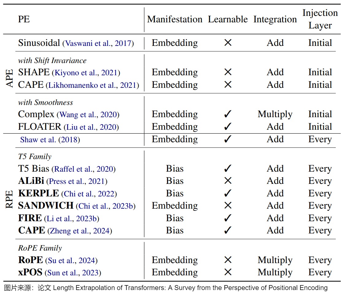
The owner question is:

When a model is asked to process positions, distances, and dependency spans outside its training distribution, which coordinate, attention, training, cache, and evaluation changes are required for useful context rather than a merely larger accepted input?

M3.5 owns the model-level extension recipe and evidence. M4 owns kernel cost. M5 owns multi-request memory and scheduling. A context extension is not complete until all three boundaries agree, but this article does not duplicate their implementation internals.

The ownership firewall is more precise than a topic list:

Article	Object it owns	What M3.5 consumes or hands off
M3.3	where absolute rows, relative terms, and score biases enter attention	consumes the insertion point; does not rederive each positional family
M3.4	vanilla rotary operator, pairing, layout, frequency ladder, and cache-local rotation invariants	consumes a verified position_ids -> phase -> rotated Q/K operator
M3.5	changes intended to extend usable context, their adaptation state, and evidence contract	owns interpolation, frequency remapping, recurrent/summary architecture state, training, and effective-context evaluation
M4	arithmetic, traffic, kernels, parallel execution, and numerical implementation cost	hands off longer prefill/decode shapes and any extra persistent or temporary state
M5	production cache allocation, scheduling, prefix reuse, retention, and request admission	hands off an immutable position/cache identity and measured target lengths

The visual is deliberately directional. Runtime allocation cannot repair an untrained geometry, and a sound geometry cannot prove task use. Conversely, a failed long-context benchmark does not identify which earlier contract failed; that requires the tensor, training, runtime, and evaluation traces developed below.

---

Background knowledge: extrapolation is distribution shift plus systems pressure

Sequence models are trained under a length distribution, not only a maximum integer. Extending context changes several conditions at once: position values may leave the training range, attention must connect more row pairs, persistent KV state grows, and the relevant evidence may be farther from the answer.

mathematical extension:
    the formula returns values at a larger position

software extension:
    the runtime accepts and allocates the larger sequence

statistical extension:
    the model remains competent outside its training-length distribution

task extension:
    the model actually uses distant evidence under realistic distractors

Long-context methods change different members of this stack. A position-scaling method cannot by itself solve memory pressure, and a larger cache allocation cannot teach the model to reason over evidence it never learned to use.

0x00A Context extension is a joint model-and-system intervention

The A23 source surveys two broad ways to improve length generalization:

extrapolatable positional mechanisms:
    design coordinates or score biases whose rule remains useful at new lengths

position-extension interventions:
    remap positions/frequencies and adapt an existing checkpoint

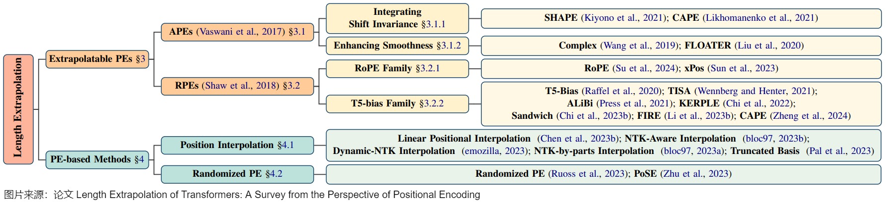
That distinction is operational. Training a model from scratch with ALiBi is not the same intervention as loading a RoPE checkpoint and changing its base. Likewise, Position Interpolation changes an existing coordinate map, while randomized position training changes the distribution of coordinates observed during optimization.

The complete dependency chain is:

coordinate map
    -> Q/K or score geometry
        -> learned attention patterns
            -> training examples and objectives
                -> kernel work and numerical behavior
                    -> persistent KV state
                        -> task evidence actually used

An extension can fail at any arrow. This motivates five independent proof obligations:

Obligation	Evidence required
representation	new positions produce defined, compatible coordinate objects
optimization	adaptation exposes the model to the new distance/task distribution
numerical	phases, masks, softmax, and kernels remain stable at target length
systems	prefill, decode, and KV memory fit the deployment budget
behavioral	quality depends correctly on distant evidence under distractors

Reporting only perplexity or only a maximum accepted token count leaves most of the claim unaudited.

Interpolation, extrapolation, and recurrence are different levers

direct extrapolation:
    evaluate the original coordinate function at unseen positions

interpolation:
    map a larger physical range into a coordinate range closer to training

frequency redesign:
    change how local and global phase resolution is allocated across dimensions

relative bias:
    define a pairwise distance function that continues at new offsets

recurrence or external memory:
    change which historical state is available without representing one full
    dense sequence in the original coordinate range

The last category changes both the model graph and runtime state. M3.5 owns the architecture-level reason that recurrence extends reachable history; M5 owns how persistent state is allocated, moved, admitted, and retired in a serving system. Keeping that split explicit prevents “long context” from being reduced to either one RoPE flag or one larger cache allocation.

Architecture-level extension: Transformer-XL segment recurrence

Independent fixed-length segments create two failures at once. No forward state crosses a segment boundary, so a dependency cannot extend beyond the segment. The first rows of every new segment also lose their left context even when the boundary was introduced only for batching. Transformer-XL changes the architecture by reusing prior hidden-state rows as a detached memory for the next segment.

Let the current segment contain L rows, let the retained memory contain M rows, and let layer n - 1 expose

$$H_{\tau}^{n-1}\in\mathbb{R}^{B\times L\times d}, \qquad M_{\tau}^{n-1}\in\mathbb{R}^{B\times M\times d}.$$

The extended source for the layer is

$$\widetilde H_{\tau}^{n-1} = \left[ \operatorname{SG}\!\left(M_{\tau}^{n-1}\right) \,;\, H_{\tau}^{n-1} \right] \in\mathbb{R}^{B\times(M+L)\times d},$$

where SG is stop-gradient and the semicolon concatenates rows along the sequence axis. Queries come only from current rows, while keys and values come from both retained and current rows:

$$Q_{\tau}^{n}=H_{\tau}^{n-1}W_Q^n, \qquad K_{\tau}^{n}=\widetilde H_{\tau}^{n-1}W_K^n, \qquad V_{\tau}^{n}=\widetilde H_{\tau}^{n-1}W_V^n.$$

After splitting into n_h heads, the important shapes are

Q:       [B, n_h, L,     d_h]
K, V:    [B, n_h, M + L, d_h]
scores:  [B, n_h, L,     M + L]
output:  [B, n_h, L,     d_h]

The asymmetry is the mechanism, not a shape accident:

1. Memory rows are historical context, so the layer does not need to emit new outputs or losses for them. They therefore do not contribute query rows.
2. A current query may retrieve content from retained history or from its causal prefix in the current segment, so both regions contribute K/V rows.
3. Stop-gradient preserves the forward dependency while bounding the backward graph at the segment boundary.

Stop-gradient does not freeze the current projection parameters. A detached memory row is still multiplied by the current W_K and W_V, so gradients can update those matrices. What disappears is the gradient path into the earlier computation that originally produced the memory row.

The segment transition follows the Transformer-XL recurrence contract and the explanatory sequence in the book’s Figure 6.15. The projection asymmetry, mask, and stored-object panels are an independent Transformer System reconstruction.

Causal mask over memory plus current rows

For zero-based current query row i, all M memory columns are historical and visible. Among current-segment columns, only rows through i are visible. With columns ordered as [memory ; current], the allowed relation is

$$\operatorname{allow}(i,j) \iff j\le M+i, \qquad i\in[0,L-1],\ j\in[0,M+L-1].$$

For M = 3 and L = 4, the mask contract is:

columns:       m0 m1 m2 | x0 x1 x2 x3
query x0:       1  1  1 |  1  0  0  0
query x1:       1  1  1 |  1  1  0  0
query x2:       1  1  1 |  1  1  1  0
query x3:       1  1  1 |  1  1  1  1

This produces L, not M + L, output rows. Treating the concatenated source as ordinary self-attention and emitting all rows would recompute historical states and duplicate prediction positions.

The recurrence moves across both segment and layer

The memory consumed by layer n is made from layer n - 1 hidden states. The cross-segment path is therefore

segment tau,     layer n - 1 hidden rows
    -> detached layer n - 1 memory
        -> segment tau + 1, layer n attention

That differs from an RNN whose state usually returns to the same recurrent layer at the next time step. In the paper’s equal-segment schematic, the largest possible dependency path grows as O(N * L) for N layers and segment length L: each segment crossing also advances one layer. This is a source-reported architecture property, not a claim that every task will use all reachable history.

Rolling memory update

The memory need not equal exactly one previous segment. A bounded M-row memory can span several segments:

$$M_{\tau+1}^{n} = \operatorname{SG}\!\left( \operatorname{tail}_{M} \left([M_{\tau}^{n};H_{\tau}^{n}]\right) \right).$$

The official PyTorch implementation stores N + 1 tensors for the embedding stream and layer outputs, uses time-major [M,B,d] layout, and performs the rolling slice under torch.no_grad() before calling .detach(). A conceptual implementation needs the layer-input memories that attention will consume; the extra final-output entry keeps the code’s hidden-state and memory lists aligned. Its ext_len path excludes overlapping rows that will be supplied explicitly on the next call:

def update_segment_memory(old_mems, current_hids, mem_len, ext_len):
    # Each tensor is time-major: [rows, batch, d_model].
    mlen = old_mems[0].shape[0]
    qlen = current_hids[0].shape[0]

    cache_end = mlen + max(0, qlen - ext_len)
    cache_begin = max(0, cache_end - mem_len)

    with torch.no_grad():
        return [
            torch.cat([old, current], dim=0)[cache_begin:cache_end].detach()
            for old, current in zip(old_mems, current_hids)
        ]

The attention-side implementation follows the same asymmetry:

extended = torch.cat([memory, current], dim=0)  # [M + L, B, d]

q = q_proj(current)                            # [L, B, n_h, d_h]
k, v = kv_proj(extended).chunk(2, dim=-1)      # [M + L, B, ...]

scores = einsum("ibhd,jbhd->ijbh", q, k)
scores.masked_fill_(causal_mask[:, :, None, None], -inf)
current_output = einsum("ijbh,jbhd->ibhd", softmax(scores, dim=1), v)

This code-level detail separates Transformer-XL memory from the ordinary autoregressive K/V cache in M5:

Contract	Transformer-XL recurrence	Ordinary decode K/V cache
stored object	unprojected hidden rows per layer input/output stream	projected K and V rows per layer
query rows	current segment	current decode/prefill rows
old-state projection	memory is reprojected into K/V on the next segment	cached K/V are normally consumed directly
training graph	prior hidden computation is detached	inference normally has no backward graph
semantic role	learned architecture-level cross-segment state	exact-prefix computation reuse for a fixed model

Calling both objects a “KV cache” hides their different state, compute, and training contracts.

Position coherence is part of the recurrence

Reusing hidden states while assigning every segment the same absolute positions 1..L creates temporal ambiguity: old and current rows can carry the same within-segment position despite being one or more segments apart. Transformer-XL therefore pairs recurrence with its relative attention parameterization. The query scores a memory/current key by relative distance, along with content and learned bias terms, instead of trusting a repeated absolute slot identity.

This is not evidence that any position method can be attached after training. The checkpoint, relative-score rule, memory order, and mask were trained as one architecture. M3.3 derives the relative-position score families; this section only establishes why position coherence is required by state reuse.

Training and runtime contract

Segment recurrence requires ordered stateful execution even though attention inside one segment remains parallel:

stream batch at segment tau
    -> current hidden rows and losses
    -> detached rolling memory per stream and layer
    -> same streams at segment tau + 1

The dataloader and runtime must therefore preserve several invariants:

• Segment order is preserved independently for every batch stream.
• Memory is reset at document or sequence boundaries unless cross-document conditioning is an explicit training policy.
• Batch sorting, admission, or eviction applies the same permutation to every layer’s memory tensor.
• Loss belongs to current target rows; cached memory rows are context, not repeated labels.
• mem_len, segment length, overlap/ext_len, relative-position range, and mask policy are checkpoint/runtime compatibility fields.
• Training and evaluation memory lengths are reported separately. The paper used a training memory equal to segment length in its experiments and tested longer memories at evaluation; that is a method-specific result, not a universal guarantee.

The state and score ledgers are now explicit. Ignoring embeddings, allocator padding, and temporary projections, a code path that stores N + 1 hidden streams uses approximately

$$M_{\text{recurrent state}} \approx (N+1)B M d\,b$$

bytes, while each layer forms

$$B\,n_h\,L(M+L)$$

attention-score elements before an IO-aware kernel changes materialization. Recurrence avoids recomputing old hidden layers from raw tokens, but it does not make historical state or current-to-memory attention free.

Failure signatures

Mistake	Observable failure
omit detach() / no_grad()	the graph grows across segments; memory and backward cost increase toward full BPTT
reinitialize memory every segment	shapes run, but cross-segment information flow disappears
store projected K/V while the layer expects hidden rows	double projection or incompatible dimensions corrupt attention
build queries for memory rows	historical positions are recomputed and may receive duplicate outputs/losses
mask memory columns as future rows	recurrence exists in storage but current tokens cannot read it
reuse local absolute positions without a coherent relative rule	different physical times become positionally ambiguous
carry memory across unrelated documents	one sample reads another document’s hidden state
reorder batch streams without reordering memory	each sequence receives another sequence’s history
increase evaluation mem_len without validation	software accepts more state, but quality and numerical behavior remain unproven

Transformer-XL therefore demonstrates an architecture-level route to longer reachable history. It does not demonstrate that a RoPE checkpoint extrapolates, and it does not settle the serving residency, paging, and admission problems owned by M5.

Architecture-level extension: accumulated learned segment summaries

Transformer-XL preserves bounded hidden rows from earlier segments. An AutoCompressor changes the persistent object: special learned summary-token inputs ask the model to emit final-layer hidden vectors that later segments consume as a soft prompt. This is a trained architecture and state transition, not a post-hoc K/V eviction rule.

Let segment i contain m_i token embeddings, let kappa be the number of summary tokens emitted per compressed segment, and let sigma_<i concatenate the summaries from all earlier segments. The input rows are

$$X_i = [\,\sigma_{<i};\ E(S_i);\ G\,] \in \mathbb{R}^{B\times((i-1)\kappa+m_i+\kappa)\times d_{model}},$$

where G is the learned block of kappa summary-token embeddings. If the Transformer returns final hidden state H_i, the current summary is

$$\sigma_i = H_i[:,\,-\kappa:,:] \in \mathbb{R}^{B\times\kappa\times d_{model}},$$

and summary accumulation updates the persistent state as

$$\sigma_{<i+1} = [\,\sigma_{<i};\ \sigma_i\,].$$

The two similarly named objects must not be collapsed:

summary-token embedding G:
    learned input rows that request a summary

summary vector sigma_i:
    final-layer hidden rows produced at those positions

neither object:
    an original token's already-projected per-layer K/V rows

The accumulation design also differs from a fixed recurrent bottleneck:

Design	State passed to segment i	Persistent rows before segment i	Information path
fixed recurrent summaries	previous summary sigma_(i-1)	kappa	evidence is repeatedly recompressed through one recurrent state
AutoCompressor accumulation	sigma_1, ..., sigma_(i-1)	(i - 1) * kappa	each segment retains a direct summary-level path to later segments

Summary accumulation is compressed growth, not globally fixed-size memory. For b bytes per scalar, its externally stored payload before segment i is

$$M_{summary}(i) = B(i-1)\kappa d_{model}b.$$

This grows linearly in compressed segments, at kappa vectors per segment rather than m_i source-token rows. Attention over the accumulated summary prefix can still grow quadratically. A report that says only “50 summary vectors” is incomplete unless it says whether those vectors replace one segment or the entire document.

Training makes the summary state consumable

The training signal is next-token prediction on the real segment tokens while conditioning on all previous summaries:

$$\mathcal{L} = -\frac{1}{N} \sum_{i=1}^{n}\sum_{t=1}^{m_i} \log p(x_t^i\mid x_{<t}^i,\sigma_{<i}).$$

Summary positions have no target text labels. Gradients from later segment-token losses teach the summary rows what to preserve. The paper also randomizes segment lengths so the learned compression operation is not tied to one fixed boundary.

Retaining a full cross-segment graph would defeat much of the memory purpose. The reported experiments use gradient checkpointing inside segments and stop gradients through cached summary state after two compression steps. That is truncated backpropagation through the summary recurrence, not a claim that all summary vectors are globally non-differentiable.

summary_prefix = empty([batch, 0, d_model])
steps_since_detach = 0

for segment in document_segments:
    prior_summary_len = summary_prefix.shape[1]
    x = concat(
        summary_prefix,
        embed(segment),
        learned_summary_tokens,
        axis="sequence",
    )

    h = transformer(x)
    segment_h = h[:, prior_summary_len : prior_summary_len + segment.shape[1]]
    new_summary = h[:, -kappa:]

    loss += next_token_loss(lm_head(segment_h), segment)
    summary_prefix = concat(summary_prefix, new_summary, axis="sequence")

    steps_since_detach += 1
    if steps_since_detach == 2:  # Reported experimental truncation.
        summary_prefix = stop_gradient(summary_prefix)
        steps_since_detach = 0

The optimization surface is checkpoint-specific. The paper’s OPT AutoCompressors fine-tune the model with newly initialized summary embeddings. Its Llama-2 experiment instead applies rank-16 LoRA to the attention Q/K/V and output projections and also optimizes the summary-token embeddings. Adding summary tokens only at inference is therefore not a valid conversion recipe for an unchanged base checkpoint.

Position and runtime contracts

Position handling belongs to the architecture. In the reported OPT path, summary tokens and summary vectors receive no absolute position embeddings, leaving pretrained absolute positions available for segment tokens; distinct summary-token embeddings preserve their order. The RoPE-based experiment applies relative positional encoding to summary tokens and vectors normally. A summary tensor cannot move between these checkpoints without its model and position conventions.

The official implementation exposes both explicit and internal accumulation:

# Explicit compression and reuse.
out = model(context_ids, output_softprompt=True)
summary_prefix = out.softprompt
next_out = model(next_segment_ids, softprompt=summary_prefix)

# Or let the model split and accumulate internally.
out = model(long_ids, segment_lengths=[m_1, m_2, m_3])

Once sigma_i is extracted, token-level working state for segment S_i may be discarded if summaries are the architecture’s only persistent history. Later consumption still projects the d_model summary vectors into per-layer K/V for that call:

persistent between calls:
    accumulated summary vectors       [B, (i - 1) * kappa, d_model]

temporary while compressing segment i:
    segment activations, attention state, and current summary rows

created when summaries are consumed:
    per-layer K/V projected from the summary-prefix embeddings

discarded under summary-only history:
    token-addressable state for completed source segments

The failure contract is correspondingly architectural and lossy:

Failure	Consequence
summary bottleneck	evidence absent from sigma_i cannot be recovered from discarded source rows
segmentation shift	boundaries unlike training change what evidence is compressed together
unreported accumulation	persistent state silently grows by kappa rows per segment
checkpoint or position mismatch	the receiving model interprets summary rows under a different learned contract
false K/V equivalence	treating sigma_i as projected K/V bypasses the model path that consumes it

M3.5 owns this architecture, training, and position contract. M5.4 compares its persistent serving object and byte trajectory with retained K/V, while M5.5 owns any later residency, retrieval, or promotion mechanism applied to that state.

0x01 Name the lengths

The phrase “train short, test long” hides several different lengths.

Name	Meaning	Typical object
L_train	length distribution used during pretraining or context-extension fine-tuning	training data and curriculum
L_config	configured maximum length accepted by model or server	max_position_embeddings, max_model_len, max_cache_len
L_test	length used in evaluation or deployment prompt	benchmark prompt or user request
L_runtime	length actually processed by prefill, decode, attention kernels, and KV cache	score tensors and cache tensors
L_task	distance and structure required by the task evidence	document span, code dependency, tool-history event

Length extrapolation is usually written as:

$$L_{\text{test}} > L_{\text{train}}$$

But a production claim needs more fields:

The model trained mostly at 4096.
The config accepts 32768.
The server admits 32768 only if KV memory is available.
The benchmark places evidence 24000 tokens away.
The task requires comparing that evidence with a table near the end.

Those are different statements. A long prompt can be:

accepted:
    tokenizer and server allow the tokens

attended:
    attention/runtime can compute over retained tokens

used:
    the final answer correctly depends on distant evidence

Most long-context mistakes come from treating the first line as proof of the third.

---

0x02 Four ceilings

“The context length is 32k” can mean any of four ceilings.

Ceiling	Local object	Failure symptom	Debugging question
software/config	tokenizer limit, model config, server limit, cache allocation	prompt rejected or silently truncated	What length does the runtime actually admit?
position mechanism	learned table, sinusoidal formula, ALiBi bias, RoPE rotation/scaling	tensors run but quality drops after original length	What coordinate distribution did the model learn?
attention/runtime	prefill work, decode score width, KV cache bytes, active request set	OOM, high TTFT, slow TPOT, low throughput	Can the system afford the retained context?
task/evaluation	evidence distance, distractors, reasoning depth, answer extraction	model ignores early evidence or follows wrong span	Does the test require the behavior users need?

A model trained on 2048-token windows may allocate tensors for 8192 tokens. That only proves part of the software ceiling. It does not prove that the position geometry, attention patterns, cache state, and task behavior remain reliable at 8192.

Failure geometry: range, resolution, uncertainty, and use

The position ceiling itself contains several non-equivalent failures. Let $g_L(m)$ map physical token position $m$ to the coordinate used for a request of length $L$, and let $\widetilde\omega_i(L)$ be the selected inverse frequency for rotary pair $i$. Its absolute and relative phases are

$$\phi_i(m;L)=g_L(m)\widetilde\omega_i(L), \qquad \Delta\phi_i(m,n;L)=\bigl(g_L(m)-g_L(n)\bigr) \widetilde\omega_i(L).$$

That notation exposes five separate proof obligations:

Failure class	Measurable object	Typical symptom
coordinate-range OOD	$g_L(m)$ against coordinates observed during training	table lookup failure or unseen absolute coordinate
phase-range OOD	$\Delta\phi_i$ against pairwise phases observed during training	direct RoPE extrapolation wraps through unfamiliar relative geometry
resolution distortion	local slope $\partial\phi_i/\partial m$ relative to training	nearby tokens become less distinguishable after compression
attention uncertainty	entropy/margin of target attention under changed geometry	probability spreads across distractors even when phases are defined
task-use failure	controlled output dependence on distant evidence	accepted and attended context does not change the answer correctly

For a locally smooth map, define pairwise resolution relative to vanilla training geometry:

$$R_i(m;L) = \frac{\partial \phi_i(m;L)/\partial m}{\omega_i} = g_L'(m)\frac{\widetilde\omega_i(L)}{\omega_i}.$$

Vanilla direct extrapolation has $R_i=1$: local spacing is unchanged, but phase range grows beyond training. Uniform Position Interpolation by factor $s$ has $g_L(m)=m/s$ and $R_i=1/s$: phase range is compressed while local resolution shrinks in every pair. Base scaling keeps $g_L(m)=m$ but makes $R_i=\widetilde\omega_i/\omega_i$ pair dependent. YaRN and searched mappings choose different regimes across pairs; LongRoPE can also change regime across positions.

Phase wrapping alone is not a proof of failure. Rotation is periodic by design, and M3.4 derives that local operator. The extension question is whether the joint phase vector across pairs, after learned Q/K projections, remains in a regime the checkpoint can use. Two offsets can be close in one pair and far in another; approximate collisions depend on the entire ladder and learned subspace, not one cosine.

Attention uncertainty is downstream of that geometry. For attention probabilities $a_{t,j}$, a useful diagnostic is

$$H_t=-\sum_j a_{t,j}\log a_{t,j}, \qquad \gamma_t = z_{t,j^*}-\max_{j\ne j^*}z_{t,j},$$

where $j^*$ is the required evidence row in a controlled task. Higher entropy or a collapsing evidence margin can diagnose retrieval failure, but these are probes, not universal quality laws. The RoPE-attention analysis paper reports source-specific evidence connecting attention-pattern preservation and lower uncertainty with better extrapolation; M3.5 uses that as a measurement proposal, not as proof that one scalar predicts all long-context tasks.

Finally, optimization support remains separate. Coordinate augmentation can cover large $g_L(m)$ values without placing content rows far apart. Long containers can expose large distances without requiring the loss to use the distant span. A valid training record therefore needs a joint distribution over

physical sequence length
coordinate and phase regime
evidence distance
distractor structure
task dependency
loss-bearing target position

This taxonomy is the common test harness for the methods below: each method must state which failure it reduces, which distortion it introduces, and which remaining obligations require training or evaluation evidence.

---

0x03 Absolute-position table limits

Learned absolute position embeddings have the most visible boundary:

position_embeddings = nn.Embedding(max_position_embeddings, d_model)
position_vectors = position_embeddings(position_ids)

The table has shape:

position_embeddings.weight:
    [max_position_embeddings, d_model]

position_ids:
    [B, n]

The hard rule is:

position_ids.max() < max_position_embeddings

If the table has 512 rows, position 800 has no row. One can resize the table, copy rows, interpolate rows, or initialize new rows, but that only creates parameters. It does not prove the model learned what those new coordinate rows mean.

Sinusoidal absolute encodings remove the hard learned-table lookup:

$$PE(pos, 2i) = \sin\left(\frac{pos}{10000^{2i/d}}\right)$$ $$PE(pos, 2i+1) = \cos\left(\frac{pos}{10000^{2i/d}}\right)$$

The formula can produce PE(pos) for large pos, but the learned layers still trained on a finite coordinate distribution. “Formula exists” is not the same as “the model knows how to use it.”

Why additive absolute PE can become fragile after projection

With additive coordinates, one score expands into four terms:

$$q_i^Tk_j = (x_i+p_i)W_QW_K^T(x_j+p_j)^T.$$

At new positions, the model is not merely seeing a new p_i^Tp_j value. It is seeing new combinations in both content-position cross terms and the projected position-position term. Smoothness of the raw sinusoidal table does not ensure smoothness of the learned score function after arbitrary projections.

Coordinate augmentation during training

Another family changes training-coordinate exposure rather than only inference coordinates. Examples include global shifts, local jitter, scaling, and ordered subsampling from a larger position range.

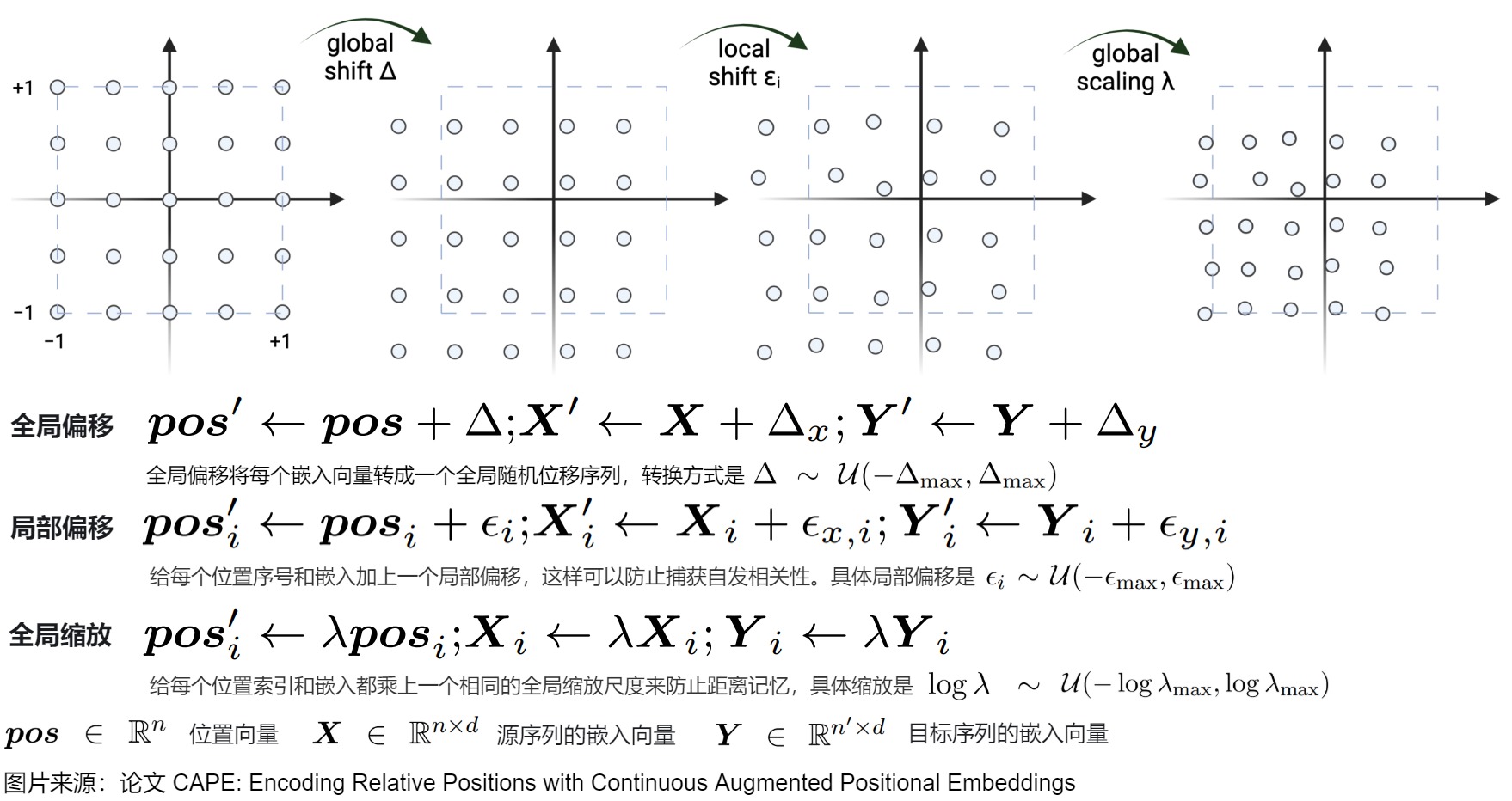
Randomized positional encoding can sample an ordered subset of positions from a larger coordinate range for each short training sequence:

def randomized_position_ids(seq_len, max_position, device):
    sampled = torch.randperm(max_position, device=device)[:seq_len]
    return sampled.sort().values

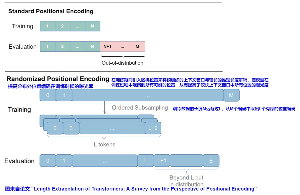
This exposes the position function to larger indices without paying full quadratic attention cost for a sequence of that physical length. It does not teach the model to connect evidence across max_position actual tokens, because only seq_len content rows are present. Coordinate-range generalization and long dependency learning remain separate.

The training contract must record whether offsets are:

global per sample:
    preserve all pairwise distances, change absolute origin

local per token:
    perturb pairwise distances as augmentation

ordered subsampling:
    preserve order, increase gaps between adjacent physical rows

global scaling:
    compress or expand every pairwise distance

These interventions are not interchangeable even if each returns position_ids: [B,N].

---

0x04 Direct extrapolation: formula exists, distribution changes

Direct extrapolation keeps the coordinate rule unchanged and asks the model to run farther.

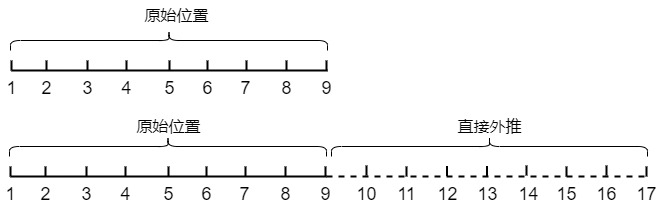
For different mechanisms, that means different things:

Method	What extends	Local warning
learned absolute	table index	hard out-of-range unless table is resized
sinusoidal	trigonometric formula	values exist, learned use may not
ALiBi	distance-proportional score bias	bias can be computed, task success is not guaranteed
RoPE	Q/K rotation angles	cos/sin exist, phase distribution changes

For RoPE, vanilla rotation uses a frequency ladder:

inv_freq = 1.0 / (
    rope_theta ** (torch.arange(0, rotary_dim, 2).float() / rotary_dim)
)

angle = position_ids[..., None] * inv_freq[None, :]
cos = angle.cos()
sin = angle.sin()

q_rot, k_rot = apply_rotary_pos_emb(q, k, cos, sin)

The Q and K shapes still match:

q, k:
    [B, h, n, d_head] or layout equivalent

q_rot, k_rot:
    same shape

The problem is semantic. At positions far beyond L_train, some dimensions rotate through phase patterns that the model did not learn to interpret. High-frequency dimensions may wrap many times. Low-frequency dimensions vary slowly. The tensors are valid, but the attention distribution may be outside the training regime.

---

0x05 RoPE object audit

M3.4 owns the RoPE proof and Q/K rotation implementation. M3.5 only needs the objects that context-extension methods change.

Object	Shape / value	M3.5 question
position_ids	[B,n]	Are positions raw, offset, compressed, or reset?
rope_theta / base	scalar	Which base produced the frequency ladder?
inv_freq	[rotary_dim/2]	Did scaling change frequency allocation?
cos, sin / freqs_cis	broadcast-compatible with Q/K	Were tables built with the same convention in train and serve?
cache_position / start_pos	scalar or [n]	Do cached keys and new queries use consistent positions?

The important mapping is:

(position_id, dimension_index)
    -> rotation angle

Config fields are just ways of defining that mapping.

Field	What to audit
max_position_embeddings	original or configured position limit
original_max_position_embeddings	denominator for scaling recipes
max_sequence_length / max_model_len	server/runtime acceptance limit
rope_theta	base for inv_freq
rope_scaling	scaling-method object
rope_type	runtime dispatch for the scaling formula
factor	PI / NTK / YaRN scaling factor
attention_factor	YaRN-style attention score correction
beta_fast, beta_slow	YaRN-style frequency-band controls
short_factor, long_factor	runtime-specific LongRoPE-style vectors, commonly one value per rotary pair
sliding_window	runtime retention policy, not a position formula
max_cache_len	cache allocation ceiling

Field names vary. The stable debugging rule is to locate the object that actually changed: position_ids, inv_freq, cos/sin, attention scaling, fine-tuning data, or cache limits.

---

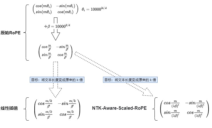
0x06 Position Interpolation: compress coordinates into the trained range

Position Interpolation changes the coordinate passed into RoPE. If the model was trained up to length $L$ and we want to run at length $L'$, define:

$$s = \frac{L'}{L}$$

Then map position $m$ to:

$$m' = \frac{m}{s}$$

The map follows directly from the endpoint requirement. If physical positions run from $0$ through $L'-1$ and the original trained coordinate interval is $[0,L)$, choose a linear map $g(m)=am$ with $g(0)=0$ and $g(L')=L$. Hence $a=L/L'=1/s$. For the last discrete position,

$$g(L'-1)=\frac{L'-1}{s}=L-\frac{1}{s}<L,$$

so every requested coordinate lies below the original continuous endpoint. This proves a range property, not a quality property.

In RoPE terms:

$$\phi(m,i) = m\theta_i$$

becomes:

$$\phi(m,i) = \frac{m}{s}\theta_i$$

scale = new_context_len / original_context_len
scaled_position_ids = position_ids.float() / scale

angle = scaled_position_ids[..., None] * inv_freq[None, :]
cos = angle.cos()
sin = angle.sin()

This compresses a long inference range into the old coordinate range.

direct extrapolation:
    m = 0 ... 8191

interpolation with s = 4:
    m' = 0 ... 2047.75

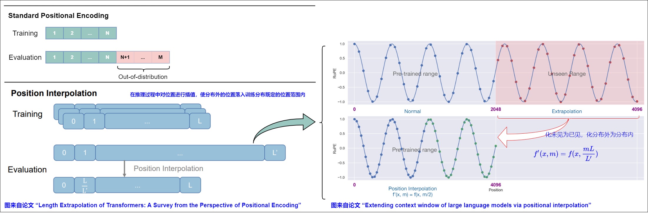
The advantage is that far positions no longer use raw coordinates outside the old range. The cost is local distortion: adjacent or nearby tokens become closer in positional phase. A distance of 4 tokens now looks like a distance of 1 token in the coordinate system.

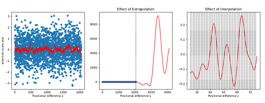
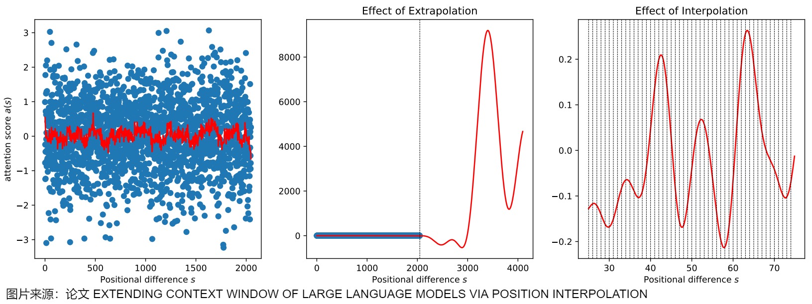
Source: Extending Context Window of Large Language Models via Position Interpolation, Figure 2. This is a constructed fitted-function example for the paper’s argument, not a measured attention trace from every long-context model. Its role is to show why “the trigonometric formula still evaluates” is weaker than “the learned score function behaves inside a familiar coordinate range.”

PI is therefore not just a harmless config flag. It changes distance semantics in every attention layer. Fine-tuning is often part of the recipe because the model has to adapt to the crowded coordinate scale.

Deriving the resolution tradeoff

For one RoPE pair with frequency theta_i, two positions separated by delta have phase difference

$$\Delta\phi_i=\delta\theta_i.$$

Uniform Position Interpolation replaces it with

$$\Delta\phi_i^{PI}=\frac{\delta}{s}\theta_i.$$

The target range grows by s, but every local phase difference shrinks by the same factor. For adjacent tokens,

$$\Delta\phi_i^{PI}(1)=\frac{\theta_i}{s}.$$

Large s can make nearby positions nearly indistinguishable in low-frequency pairs and reduce resolution even in high-frequency pairs. Fine-tuning must teach Q/K projections to interpret this denser coordinate grid.

The relative rotary score makes the same tradeoff explicit. Consuming M3.4’s pair identity,

$$\left(R(g(m))q\right)^T\left(R(g(n))k\right) =q^TR\!\left(\frac{n-m}{s}\right)k.$$

PI does not merely move two absolute endpoints. It divides every relative offset presented to every rotary pair by $s$. The phase gradient with respect to physical position is correspondingly

$$\frac{\partial\phi_i^{PI}}{\partial m}=\frac{\omega_i}{s}.$$

Backpropagation through the rotation remains ordinary differentiable tensor algebra, but the learned Q/K projections receive gradients from a different distance geometry. This is why adaptation is part of the paper’s method rather than post-hoc evidence that the same checkpoint happens to tolerate one flag.

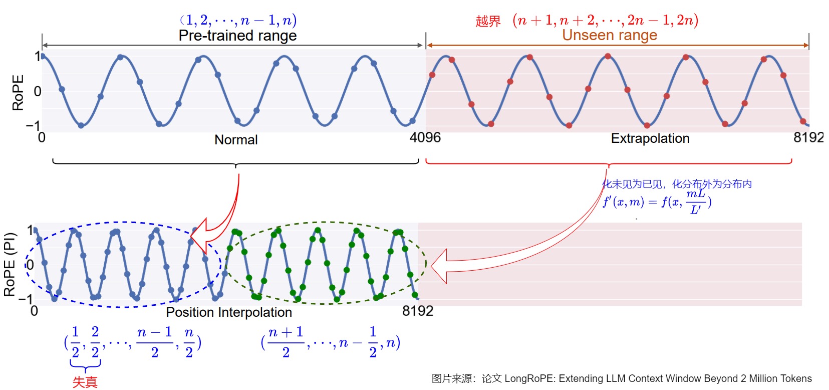
The Position Interpolation argument is not only that interpolated positions remain below the old maximum. The paper analyzes the fitted attention function between trained integer positions and argues that interpolation is better controlled than arbitrarily distant extrapolation. The visual comparison below shows the intended contrast; it remains a constructed analysis, not a guarantee for every trained Q/K function.

Training and serving must use the same coordinate implementation

Two algebraically equivalent implementations are common:

# Scale positions.
angles = (position_ids.float() / factor)[..., None] * inv_freq

# Or scale inverse frequencies.
angles = position_ids.float()[..., None] * (inv_freq / factor)

For position_ids: [B,N] and inv_freq: [d_r/2], both paths form angles: [B,N,d_r/2]. A numerically explicit implementation is:

def linear_rope_state(position_ids, inv_freq, factor, output_dtype):
    assert position_ids.ndim == 2
    assert inv_freq.ndim == 1
    assert factor >= 1.0

    # Construct phase in a controlled dtype even when Q/K are bf16/fp16.
    pos = position_ids.to(torch.float32)
    freq = inv_freq.to(device=pos.device, dtype=torch.float32) / factor
    phase = pos[..., None] * freq[None, None, :]  # [B,N,d_r/2]
    cos = phase.cos().to(output_dtype)
    sin = phase.sin().to(output_dtype)
    return cos, sin

The pinned Transformers source used by this audit implements linear scaling in _compute_linear_scaling_rope_parameters by computing the default inverse frequencies and dividing them by factor. That is an implementation trace, not a universal API promise: pin the repository commit and symbol because runtime configuration formats and dispatch code evolve.

They are equivalent only if no other method modifies position_ids or inv_freq, and if both use the same precision and factor. A checkpoint config that says factor=4 is insufficient without the runtime dispatch rule.

During decode, position m must use m/factor, not (local_decode_index)/factor. Cached keys and new queries must use the same scaled map. Prefix-cache keys also need the scaling method and original maximum in their compatibility identity.

The paper’s reported extension results include brief fine-tuning rather than a claim of universal zero-shot extension. Preserve that experimental contract:

paper claim:
    specific LLaMA checkpoints, extension factors, datasets, optimization,
    and evaluations reported by the Position Interpolation authors

local reproduction claim:
    pinned checkpoint + exact phase map + adaptation manifest + measured suite

not established by the paper alone:
    every architecture, factor, backend, workload, or no-fine-tuning setup

At minimum, a PI release test should compare: original logits with factor=1, the two equivalent phase implementations, positions around $L-1,L,L+1$, cached versus no-cache decoding, short-context regression, and quality at several intermediate lengths. Passing only the target maximum can hide a gradual loss of local resolution.

---

0x07 NTK-aware and Dynamic NTK scaling

Position Interpolation scales all frequencies uniformly by changing position_ids. NTK-aware scaling changes the RoPE base, which changes inv_freq.

The RoPE frequency ladder is:

$$\theta_i = \text{base}^{-2i/d}$$

Increasing the base makes some frequencies smaller, especially in later dimensions. That stretches wavelengths and redistributes the positional representation across frequency bands.

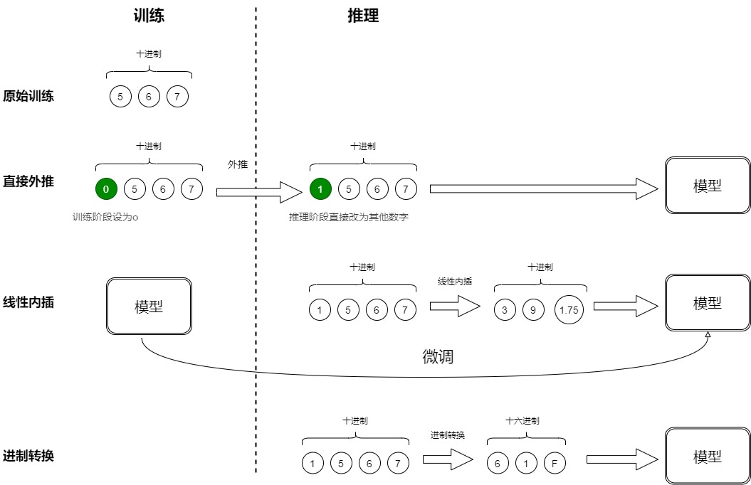
A simplified Dynamic NTK-style implementation may recompute the base when the sequence length exceeds the original maximum:

if seq_len > max_position_embeddings:
    base = rope_theta * (
        (scaling_factor * seq_len / max_position_embeddings)
        - (scaling_factor - 1)
    ) ** (rotary_dim / (rotary_dim - 2))
else:
    base = rope_theta

inv_freq = 1.0 / (
    base ** (torch.arange(0, rotary_dim, 2).float() / rotary_dim)
)

This code is an example, not a universal definition. The exact formula differs by implementation and paper. The local M3.5 point is stable:

changed object:
    inv_freq via base

shape preserved:
    Q/K rotations still return the same Q/K shape

semantic change:
    dimension bands see different phase distributions

serving risk:
    prefill and decode must use compatible scaling

If the prompt keys were cached under one inv_freq rule and the new query is rotated under another, the score tensor still has the right shape but the geometry is inconsistent.

Deriving why changing the base is not uniform interpolation

Let original inverse frequency be

$$\theta_i=b^{-2i/r}.$$

If the base becomes b' = b * c, then

$$\theta_i' =(bc)^{-2i/r} =\theta_i c^{-2i/r}.$$

The scale factor depends on pair index i. Pair zero is unchanged; later pairs are reduced progressively. In contrast, PI uses

$$\theta_i^{PI}=\frac{\theta_i}{s}$$

for every pair. This is the core reason base scaling can preserve more high-frequency local phase than uniform interpolation while stretching lower frequencies more strongly.

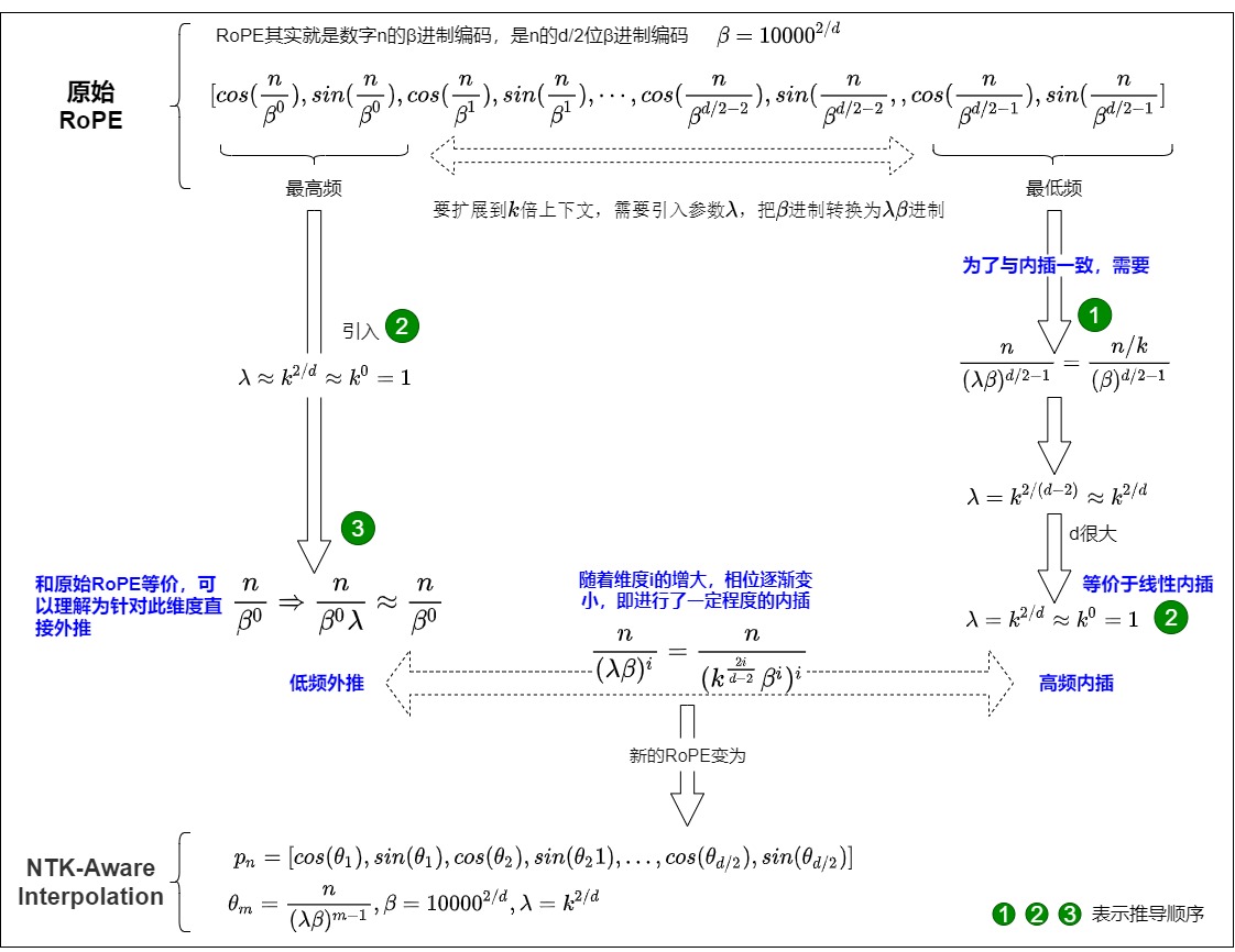
The common exponent r/(r-2) in one NTK-aware recipe is chosen so the lowest frequency pair receives approximately the desired extension factor. For the last pair i=r/2-1, the base exponent is

$$\frac{2i}{r}=\frac{r-2}{r}.$$

If

$$b'=b\,s^{r/(r-2)},$$

then the last inverse frequency becomes

$$\theta_{last}' = \theta_{last} \left(s^{r/(r-2)}\right)^{-(r-2)/r} = \frac{\theta_{last}}{s}.$$

The lowest-frequency pair is stretched by s, while earlier pairs receive less stretching. This derivation explains the formula; it does not establish a universal best runtime recipe.

For that common static parameterization, the effective frequency ratio for pair $i$ is

$$\frac{\omega_i'}{\omega_i} =s^{-2i/(r-2)}.$$

Pair zero has ratio one, the last pair has ratio $1/s$, and intermediate pairs follow a geometric schedule. The phrase “preserves high frequencies” therefore means relative to uniform PI, not that every pair is unchanged.

Static and dynamic base selection

static NTK-aware:
    choose one extended base for the checkpoint/runtime target length

dynamic NTK:
    derive the base from the current sequence length after a threshold

Dynamic selection can preserve the original map for short prompts, but creates a cache consistency problem if the base changes after K rows were already rotated. A safe implementation must define whether:

the base is fixed for the whole request at admission time;
historical K is recomputed when the threshold changes;
or the method's exact formula guarantees compatible cached phases.

Merely recomputing inv_freq when seq_len grows does not repair old rotated K. Runtime code and cache format must be audited together.

Pinned Dynamic NTK source trace

The pinned Transformers implementation used here first clamps seq_len to at least max_position_embeddings. With configured factor $s$, original length $L_0$, and rotary width $r$, it defines

$$F(\ell)=s\frac{\ell}{L_0}-(s-1), \qquad b(\ell)=b_0F(\ell)^{r/(r-2)}.$$

Therefore

$$\frac{\widetilde\omega_i(\ell)}{\omega_i} =F(\ell)^{-2i/(r-2)}.$$

At $\ell=L_0$, $F=1$ and the original ladder is recovered. Beyond that threshold, pair zero remains unchanged and the last pair is divided by $F(\ell)$. Notice that the config factor is an input to a length-dependent formula; it is not generally equal to the final per-pair stretch. This is why copying the scalar between libraries without pinning the formula is unsafe.

The source decorator has two mutable transitions:

growth:
    if request max position exceeds max_seq_len_cached
    recompute inv_freq for the new seq_len
    replace the non-persistent buffer

reset:
    if a later request returns below original_max_seq_len
    restore original_inv_freq for short-sequence precision

That source behavior is sufficient to produce frequencies for a forward call; it does not by itself prove compatibility with an external rotated-key cache. Suppose rows $0{:}t$ were rotated under ladder $\omega^{(a)}$ and growth at $t+1$ selects $\omega^{(b)}$. A score against an old row becomes

$$\left(R((t+1)\omega^{(b)})q\right)^T \left(R(j\omega^{(a)})k_j\right),$$

which cannot be reduced to the intended single-ladder relative offset unless the two ladders agree. Three valid runtime strategies are possible:

Strategy	Cache action	Tradeoff
freeze at admission	choose one target ladder before prefill and keep it for the request	stable cache; request target length must be known
rerotate/recompute	retain raw K or recompute historical K when the ladder changes	exact selected geometry; extra state or work
no cross-regime cache reuse	restart prefill when the dynamic regime changes	simple correctness; potentially large latency

“Update inv_freq and continue” is not a fourth strategy. If a framework or model defines another cache-compatible rule, that rule must be stated and tested explicitly. Shared mutable RoPE state also needs request isolation: a short request resetting the buffer must not change the ladder used by an in-flight long request.

Required probes are: $L_0-1,L_0,L_0+1$; growth past every cached maximum; return to a short request; one-shot versus token-by-token decoding; cached versus recomputed logits; and interleaved short/long request execution on the same model instance.

---

0x08 YaRN, LongRoPE, Giraffe, and mixed recipes

Mixed schemes exist because not all dimensions want the same treatment. High-frequency dimensions carry local detail. Low-frequency dimensions change slowly and can support long-range structure. A single uniform rule can help long range while damaging local resolution.

Use method names as audit handles, not as a memorization list.

Family	Changed object	Claimed goal	Audit fields	Common failure
NTK-by-parts	frequency-band scaling	preserve local resolution while extending low-frequency range	band split, scale per band	wrong band thresholds
YaRN	frequency-band scaling, attention_factor, fine-tuning recipe	efficient RoPE context extension with short-context retention	factor, attention_factor, beta_fast, beta_slow	missing attention correction or short-context regression
LongRoPE	per-dimension factors, initial-position threshold, progressive extension, short-context readjustment	extend very far while recovering short windows	factor vector, start threshold, short/long dispatch, progressive training	runtime lacks the exact mapping or loads factors in the wrong order
Giraffe	basis/scaling/truncation experiments and task evaluation	study context expansion recipes beyond perplexity	base, scaling, training/eval mix	benchmark claim does not match task

The unifying question is:

what function maps position_ids and dimension index to rotation angle?

For ordinary RoPE:

$$\phi(m,i) = m\theta_i$$

For PI:

$$\phi(m,i) = \frac{m}{s}\theta_i$$

For NTK-aware scaling:

$$\phi(m,i) = m\theta_i'$$

For mixed schemes:

$$\phi(m,i) = f(m,i)$$

where $f$ may depend on frequency band, scaling regime, attention correction, and fine-tuning target.

YaRN: preserve, interpolate, or blend by wavelength

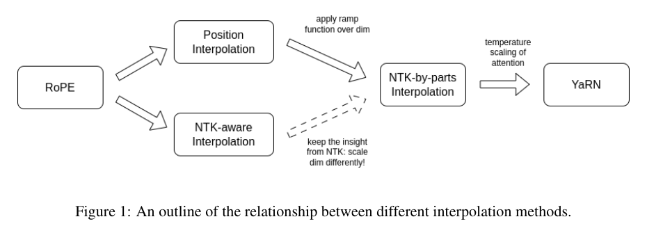
Source: YaRN: Efficient Context Window Extension of Large Language Models, Figure 1. The diagram is a dependency map for YaRN’s recipe, not a claim that every runtime implements the same fields or formulas. Audit the actual frequency ramp and attention scaling separately.

YaRN builds on the NTK-by-parts observation that uniform PI compresses local phase differences in every rotary pair. Let theta_i be the original inverse frequency, s the extension factor, and define a high-frequency preservation weight g_i:

$$g_i = \begin{cases} 1, & \text{high-frequency pair: preserve} \\ 0, & \text{low-frequency pair: interpolate} \\ (0,1), & \text{transition band} \end{cases}$$

A compact implementation-level description is:

$$\theta_i^{\text{YaRN}} = g_i\theta_i + (1-g_i)\frac{\theta_i}{s}$$

high frequency / short wavelength:
    theta_i' = theta_i
    preserve nearby-token phase resolution

low frequency / long wavelength:
    theta_i' = theta_i / s
    compress the long coordinate range

middle frequencies:
    blend the two rules with a ramp

beta_fast and beta_slow are implementation/config controls for locating that transition from a frequency’s rotations or wavelength relative to the original context. Their names do not define a universal tensor formula; the runtime’s RoPE function does.

The usual correction-dimension formula can be derived from the number of full rotations a pair makes over the original training length $L_0$. For pair index $i$ and base $b$:

$$\theta_i=b^{-2i/r}, \qquad \operatorname{rotations}_i =\frac{L_0\theta_i}{2\pi}.$$

Set this count to a boundary value $\beta$ and solve for $i$:

$$\beta=\frac{L_0b^{-2i/r}}{2\pi},$$ $$\log\left(\frac{L_0}{2\pi\beta}\right) =\frac{2i}{r}\log b,$$ $$i(\beta) =\frac{r\log(L_0/(2\pi\beta))}{2\log b}.$$

beta_fast and beta_slow map to two correction dimensions. After clamping them to valid pair indices, a linear ramp can define the blend:

def correction_dim(rotations, rotary_dim, base, original_length):
    return (
        rotary_dim
        * math.log(original_length / (2 * math.pi * rotations))
        / (2 * math.log(base))
    )

lo = floor(correction_dim(beta_fast, ...))
hi = ceil(correction_dim(beta_slow, ...))
ramp = ((pair_index - lo) / max(hi - lo, eps)).clamp(0, 1)

Different codebases orient ramp in opposite directions and may swap the names of interpolation/extrapolation weights. The conformance test is the resulting frequency behavior:

designated fast/high-frequency pairs:
    remain near original theta_i

designated slow/low-frequency pairs:
    approach theta_i / s

Auditing only beta_fast < beta_slow is insufficient because the correction dimension decreases as requested rotation count increases.

For a concrete source trace with $r=128$, $b=10000$, $L_0=4096$, beta_fast=32, and beta_slow=1, the unrounded correction dimensions are approximately

i(beta_fast = 32) = 20.944...
i(beta_slow = 1)  = 45.027...

The pinned Transformers implementation truncates these to a ramp interval [20, 46]. It constructs an increasing ramp over the 64 rotary pairs, then uses 1 - ramp as the extrapolation/original-frequency weight:

pair index <= 20:
    original inverse frequency; local high-frequency resolution preserved

20 < pair index < 46:
    convex blend of original and divided-by-factor frequency

pair index >= 46:
    interpolated inverse frequency; long wavelengths stretched by factor

This numeric trace resolves the naming trap. In this implementation, lower pair indices are the faster frequencies, and inv_freq_extrapolation_factor means “weight on the original frequency,” not “weight on PI.” A port can use opposite variable names and still be correct; compare the output ladder.

The second YaRN object is not inv_freq. The paper adds a temperature-like correction to attention logits:

$$P = \operatorname{softmax}\left( \frac{1}{t} \frac{Q'K'^T}{\sqrt{d_h}} \right)$$

The paper notes that this can be implemented by scaling the rotary embeddings, which changes the Q/K dot-product magnitude without rewriting the attention kernel. Modern configs often expose the corresponding quantity as attention_factor. Exact parameterization varies: inspect whether the runtime scales cos/sin, Q/K, or scores, and whether the factor is applied once or effectively squared through both Q and K.

So a YaRN audit has two independent checks:

frequency mapping:
    theta_i -> theta_i^YaRN

attention magnitude:
    q_rot @ k_rot.T -> corrected score scale

Loading the band schedule while dropping the attention correction is not the same method. Applying the correction twice is also wrong even though every shape survives.

The square is the implementation trap. If the desired score multiplier is $\kappa$,

$$s'=\kappa\frac{q'^Tk'}{\sqrt{d_h}},$$

and the runtime instead scales both rotary outputs by $a$, then

$$(aq')^T(ak')=a^2q'^Tk'.$$

Therefore $a=\sqrt\kappa$. For a softmax temperature $t$, where the desired score multiplier is $1/t$, the symmetric Q/K scale is $a=t^{-1/2}$. A config field called attention_factor may mean $a$, $a^2$, or a paper-specific intermediate depending on the implementation. Verify the final score ratio on a fixed Q/K tensor rather than trusting the field name.

base_score = q_rot @ k_rot.transpose(-2, -1)
scaled_score = (a * q_rot) @ (a * k_rot).transpose(-2, -1)
torch.testing.assert_close(scaled_score, (a * a) * base_score)

In the pinned Transformers path, the default returned factor is

$$a(s)= \begin{cases} 1,&s\le1,\\ 1+0.1\log s,&s>1, \end{cases}$$

unless explicit attention_factor or compatible mscale fields override it. For $s=8$, $a\approx1.207944$; multiplying both cos and sin by this value scales rotated Q and K by $a$ and their score contribution by $a^2\approx 1.45913$. Do not compare a config field directly with a paper temperature without tracing where it enters the model.

YaRN’s paper reports, for its studied checkpoints and setup, lower adaptation token and step requirements than prior approaches. Those are source-reported experimental results, not constants of the frequency formula. A reproduction must preserve:

base checkpoint and original context
extension factor and complete frequency-band configuration
attention-factor convention and application site
training length mixture, token count, steps, optimizer, and data
short-context and target-context evaluations
runtime source/version used for derived frequencies

A zero-training runtime experiment is a different method contract even if it uses the same YaRN frequency function.

LongRoPE: search a factor per rotary pair and a position threshold

LongRoPE makes the interpolation rule non-uniform over both rotary dimensions and token positions. In the paper’s local notation, let lambda_i be a searched rescale factor for rotary pair i, and let n_hat be the number of initial positions kept on original RoPE. The angle map is:

$$\phi(n,i) = \begin{cases} n\theta_i, & n < \hat{n} \\ \dfrac{n\theta_i}{\lambda_i}, & n \ge \hat{n} \end{cases}$$

The changed objects are therefore:

lambda:
    [rotary_dim / 2]
    one rescale factor per rotary pair

n_hat:
    scalar threshold
    initial positions use unscaled RoPE

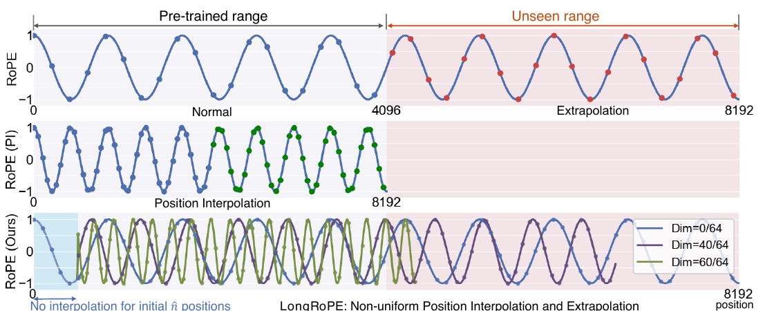
Source: LongRoPE: Extending LLM Context Window Beyond 2 Million Tokens, Figure 2. The bottom panel visualizes two independent non-uniformities: different rotary dimensions receive different factors, and the first n_hat positions can remain unscaled. It illustrates the mapping; the paper’s large extension result also depends on search, staged adaptation, and short-context recovery.

The paper searches these objects using long-sequence perplexity, with a monotonic constraint on the per-dimension factors to reduce the search space. This is different from deriving every factor from one scalar rope_theta or one uniform factor.

LongRoPE’s very large extension claim also depends on a staged recipe, not just the angle equation:

stage 1:
    search an extension mapping for an intermediate window
    fine-tune at that intermediate length (256k in the paper recipe)

stage 2:
    search another mapping on the extended checkpoint
    use the non-uniform interpolation to reach the larger target

short-window recovery:
    search/readjust factors for short inputs
    dispatch to the short-context mapping below its threshold

Checkpoint schemas may serialize this last distinction as short_factor and long_factor vectors. Those field names are a runtime representation, not the paper’s whole algorithm. A safe conceptual dispatch is:

factors = short_factors if seq_len <= short_window else long_factors
# factors: [rotary_dim // 2]
angles = position_ids[..., None] * inv_freq[None, :] / factors[None, :]

The actual threshold and formula must come from the checkpoint/runtime contract. Using the right numbers with the wrong dimension order, rotary pairing, or short/long branch produces valid cos/sin tensors with the wrong geometry.

LongRoPE’s threshold is a piecewise phase rule

The primary-paper equation applies the original angle for $n<\hat n$ and the scaled angle $n\theta_i/\lambda_i$ for $n\ge\hat n$. Unless $\lambda_i=1$, that piecewise rule can jump at the threshold:

$$\phi(\hat n^- ,i)\approx\hat n\theta_i, \qquad \phi(\hat n,i)=\frac{\hat n\theta_i}{\lambda_i}.$$

Do not silently replace it with a continuous alternative such as

$$\hat n\theta_i+\frac{(n-\hat n)\theta_i}{\lambda_i}$$

because that is a different map, even if it looks aesthetically preferable. The searched parameters are optimized under the paper’s declared piecewise rule.

The search objective can be written schematically as

$$(\lambda^*,\hat n^*) =\arg\min_{\lambda,\hat n} \frac{1}{|\mathcal X|} \sum_{x\in\mathcal X} \operatorname{NLL} \left(x;\operatorname{RoPE}_{\lambda,\hat n}\right).$$

The result is checkpoint-specific. A vector found for one base model, rotary dimension, pairing convention, or adaptation stage is not a universal LongRoPE vector.

Implementation state should expose at least:

original context length
target context length / dispatch threshold
rotary_dim and pairing convention
short_factor [rotary_dim/2]
long_factor  [rotary_dim/2]
n_hat or equivalent position regime
attention scaling, if any
training/search stage that produced each vector

If a request chooses its short/long factor from total sequence length, the choice must be fixed before cache creation or old K rows must be recomputed. Switching factor vectors after prefill changes every historical phase.

Paper map, searched artifact, and runtime representation

These three objects must not be collapsed:

LongRoPE paper search space:
    lambda[pair] plus an initial unscaled-position threshold n_hat

searched/adapted artifact:
    factors selected for one checkpoint, target, search corpus, and stage

pinned Transformers longrope runtime:
    select short_factor or long_factor for the whole request
    inv_freq_i = 1 / (factor_i * base^(2i / rotary_dim))
    return one attention_factor

The pinned runtime function does not apply the paper’s per-position n_hat branch inside one request. Its decorator switches factor vectors according to whether the request’s maximum position exceeds original_max_position_embeddings. That can be a valid serialization for a particular released checkpoint, but it is not a line-by-line implementation of the complete paper search equation. Reproduction claims must say which object they implement.

The official LongRoPE repository exposes evolutionary-search machinery and states that general training systems can be used for the adaptation stages. Consequently, “ran the repository” does not by itself reconstruct the paper’s progressive fine-tuning. Record population initialization, monotonic factor constraint, mutation/crossover settings, search samples, perplexity reduction, selected vector, and every training checkpoint between searches.

LongRoPE2: a different search and training contract

LongRoPE2 retains per-dimension rescaling but changes the diagnosis, objective, and adaptation schedule. The paper first defines a theoretical critical pair from whether a frequency completes a period within the original length. In pair index notation,

$$i_{tcd} = \left\lceil \frac{r}{2}\log_b\left(\frac{L_{train}}{2\pi}\right) \right\rceil.$$

It then advances a source-reported hypothesis: slowly rotating pairs may be effectively under-trained because real data seldom supplies dependencies across their full theoretical period, so the practical critical boundary can occur earlier. This is an empirical model of the paper’s results, not a theorem that every checkpoint has the same shifted boundary.

The search signal addresses a weakness of ordinary token-average perplexity. Let $I_{needle}$ contain only answer-token positions whose prediction requires the distant inserted evidence. Needle-driven negative log-likelihood is

$$\mathcal L_{needle}(\lambda) =- \frac{1}{|I_{needle}|} \sum_{t\in I_{needle}} \log p_{\lambda}(x_t\mid x_{<t}).$$

The evolutionary search uses controlled long-distance samples, searches a candidate practical critical dimension and factors above it, and applies an NTK-style schedule below that boundary. This objective is more targeted than whole-document perplexity, but it can overfit the synthetic needle generator; the selected map still needs independent retrieval, reasoning, language-model, and short-task evaluation.

LongRoPE2’s second object is mixed-window training:

long branch:
    long documents packed to target length
    rescaled RoPE
    cross-token attention allowed by the long-example structure

short branch:
    short documents packed into the same physical training length
    original RoPE
    block-diagonal document mask prevents cross-document attention

shared update:
    both branches update the same model weights

At inference, the paper dispatches original RoPE within the short context and rescaled RoPE beyond it. Therefore the release includes two positional regimes, the threshold, and weights jointly trained under both. A heterogeneous batch must preserve per-request regime identity, and a prefix created under one regime cannot be reused under the other merely because token IDs match.

All LongRoPE and LongRoPE2 scale, effective-context, and short-retention numbers remain source-reported. They transfer only with the checkpoint, factor vectors, search/training manifests, runtime semantics, and evaluation protocol that produced them.

Giraffe as an evaluation and design-space boundary

Giraffe studies several basis and scaling choices and evaluates more than one language-modeling statistic. M3.5 uses it as a warning against collapsing the design space into one “best base” value or treating perplexity as a complete usable-context test. It does not need another full RoPE derivation here.

Llama 3’s wavelength-banded fixed schedule

The pinned Transformers implementation for the Llama 3.1-style schedule starts from vanilla inverse frequencies and computes each wavelength

$$\Lambda_i=\frac{2\pi}{\omega_i}.$$

Given original context $L_0$, extension factor $s$, and two controls $c_{low}<c_{high}$, it defines wavelength boundaries

$$\Lambda_{low}=\frac{L_0}{c_{low}}, \qquad \Lambda_{high}=\frac{L_0}{c_{high}}.$$

The resulting rule is:

Wavelength region	Frequency action	Local interpretation
$\Lambda_i<\Lambda_{high}$	preserve $\omega_i$	fast/local frequency remains unchanged
$\Lambda_i>\Lambda_{low}$	use $\omega_i/s$	slow/global frequency is stretched
between boundaries	smooth blend of $\omega_i$ and $\omega_i/s$	avoid a hard pair-index transition

For the middle band, the pinned source computes

$$\alpha_i = \frac{L_0/\Lambda_i-c_{low}}{c_{high}-c_{low}}, \qquad \widetilde\omega_i = \alpha_i\omega_i+(1-\alpha_i)\frac{\omega_i}{s}.$$

This resembles YaRN’s preserve/blend/interpolate structure, but it is not YaRN: the boundary variables, default values, attention correction, and training lineage differ. The implementation returns attention factor one. Treat rope_type=llama3 as a distinct fixed frequency map and compare its derived tensor rather than translating fields by name.

CLEX: learn continuous frequency dynamics

CLEX unifies position scaling and frequency scaling by writing a length-conditioned frequency basis

$$\boldsymbol\omega(t) = \boldsymbol\alpha(t)\odot\boldsymbol\omega(1), \qquad \mathbf z(t)=\log\boldsymbol\omega(t).$$

Uniform PI is the special case $\boldsymbol\alpha(t)=1/t$ in every pair; power-law base scaling uses pair-dependent components. CLEX models the continuous evolution instead:

$$\frac{d\mathbf z(t)}{dt} = g_{\varphi}(\mathbf z(t),t), \qquad \mathbf z(t') = \mathbf z(1)+\int_1^{t'}g_{\varphi}(\mathbf z(t),t)\,dt.$$

The ODE parameters $\varphi$ are learned checkpoint state. The paper uses a lightweight up/down projection and a length-factor embedding, samples $t'\in[1,t_{train}]$ during training, and changes positional exposure so the selected frequency basis is paired with compatible coordinate ranges. Inference can precompute bases at discrete factors and choose a nearest upper bucket for a request.

That creates a different lifecycle from scalar RoPE scaling:

checkpoint:
    base model weights + learned ODE parameters

training state:
    sampled length factor + coordinate-sampling policy

runtime state:
    ODE solver/version or cached factor-to-frequency table
    bucket-selection rule fixed for the request

cache identity:
    selected frequency bucket + table/ODE artifact hash

CLEX’s paper reports extrapolation results for its models and protocol. Those numbers are source-reported; a learned continuous map does not guarantee arbitrary extrapolation, and discrete runtime bucketing reintroduces boundaries that need neighborhood tests.

M3.4 handoff acceptance: trained rotary variants

M3.4 owns the operator and checkpoint identity of learned frequencies, p-RoPE, and HoPE. M3.5 accepts only their extension-evidence question: what training regime, tested lengths, tasks, metrics, and short-context regressions support a claim beyond the training window? Accepting that handoff does not turn any of these trained architectures into a post-hoc inference switch.

M3.4 handoff	M3.4-owned change	M3.5 acceptance and evidence status
generic learned frequencies	trainable rotary parameters, optimizer state, and checkpoint/cache identity	No generic extrapolation guarantee follows from making frequencies trainable. M3.5 evaluates only a named method with a frozen training and length protocol. CLEX is one such specific method: it learns continuous frequency-basis dynamics rather than standing for every learned-frequency design.
p-RoPE	the selected lowest-frequency blocks become position independent and the retained fraction $p$ becomes part of the trained operator	The source paper reports 2B-parameter models trained and evaluated at an 8k context, then explicitly leaves careful long-context evaluation to future work. M3.5 therefore records p-RoPE as an extension hypothesis requiring new long-context evidence, not as an established extension baseline.
HoPE	paper-selected activated and low-frequency components become position independent while high-frequency rotary signals remain	M3.5 accepts the paper-bounded extrapolation claim only with HoPE’s from-scratch training and reported evaluation protocol. Its results, including combinations with PI or YaRN, do not validate toggling HoPE on vanilla RoPE weights.

The owner split is therefore exact: M3.4 answers which positional operator and state changed; M3.5 answers whether a declared protocol demonstrates useful behavior outside its training-length regime. Similar identity subspaces do not merge p-RoPE and HoPE into one method, and the phrase “learned frequencies” is not evidence until it names a concrete parameterization and evaluation bundle.

xPos: add opposite query/key magnitude scaling to rotation

xPos starts from the same rotational relative-offset identity but multiplies query and key rotary components by reciprocal position-dependent scales. In a schematic pair-wise form,

$$q_m' = R_m q_m \odot \zeta^m, \qquad k_n' = R_n k_n \odot \zeta^{-n}.$$

Their dot product contains a displacement-dependent scale:

$${q_m'}^Tk_n' \propto q_m^TR_{n-m}k_n \odot \zeta^{m-n}.$$

The reciprocal Q/K factors are essential. Applying the same factor to both sides changes the score according to m+n, not only m-n. Unlike vanilla RoPE, xPos is not norm preserving; its scaling is part of the length behavior and numerical contract.

This is an example of an architecture designed for extrapolation rather than a post-hoc uniform position remap. It must be trained with the scaling rule.

Architecture alternatives change the state graph

Frequency remapping is only one design family. The recurrence and summary mechanisms introduced earlier change which rows survive:

Family	Persistent model object	Training requirement	Runtime consequence	Main loss of equivalence
Transformer-XL	detached prior hidden rows at each layer	segment recurrence plus relative-position contract	bounded recurrent memory is concatenated to current K/V sources	not equivalent to one dense full-sequence forward
accumulated summaries	learned summary vectors in model space	summary-token objective and segmented curriculum	summary rows persist; token-level history may be discarded	lossy compression can remove unrecoverable evidence
xPos	reciprocal Q/K magnitude basis plus rotation	train the attention operator with xPos	cache identity includes scale and phase rule	not a post-hoc norm-preserving RoPE flag
CLEX	learned length-to-frequency dynamics	jointly learn model and ODE over sampled factors	derive/cache a frequency basis per request bucket	learned dynamics and bucket dispatch are new checkpoint/runtime state
fixed banded maps	deterministic factor schedule	architecture-specific adaptation or pretraining evidence	one derived frequency tensor per declared regime	config names do not establish tensor equivalence

These methods can be combined, but combination multiplies contracts. A learned frequency map plus summary memory needs both checkpoint states, coherent positions for summary rows, training under the combined graph, and an evaluation that distinguishes failure of compression from failure of position geometry.

Method comparison by changed object

Method	Position map	Frequency map	Score magnitude	Learned/searched state	Typical adaptation
direct RoPE	m	original	original	none	none
PI	m/s	uniform theta/s equivalent	original unless separately corrected	scalar factor	short long-context fine-tune commonly used
static NTK-aware	m	changed base, pair-dependent scaling	original	target factor/base	optional, runtime-specific
Dynamic NTK	m	base depends on request length	original	formula/config	cache policy required
YaRN	m	preserve/blend/interpolate by band	explicit attention correction	factor, band controls	context-extension fine-tune
LongRoPE	m	searched factor per pair and position regime	recipe-specific	vectors plus threshold	staged search/fine-tuning and short recovery
LongRoPE2	short/long regime dispatch	searched factors around a practical critical dimension	regime-specific	needle-guided search artifact	mixed original/rescaled-RoPE training
xPos	m	rotation plus reciprocal scale basis	displacement-dependent	fixed scale rule	train with architecture
Llama 3 schedule	m	preserve/blend/scale by wavelength	original	fixed band controls	checkpoint-specific training lineage
CLEX	m plus sampled coordinate exposure	learned continuous dynamics in log-frequency space	model-specific	ODE parameters or derived basis table	train across sampled length factors
ALiBi	no rotary map	n/a	linear head-specific bias	deterministic slopes	train with architecture
randomized PE	sampled ordered positions	base method unchanged	base method unchanged	sampling policy	train under augmented positions

The table prevents a common error: two methods can advertise the same target length while changing completely different tensors and requiring different checkpoint/runtime support.

---

0x09 Fine-tuning and data distribution

Many context-extension recipes are described as if changing the RoPE formula is the whole operation. In practice, the coordinate change often comes with adaptation.

coordinate change:
    PI, NTK-aware scaling, YaRN, LongRoPE, changed rope_theta, changed inv_freq

adaptation data:
    long documents, code files, book-like sequences, retrieval mixtures, synthetic long prompts

runtime path:
    prefill kernel, KV cache layout, cache_position, batch scheduling, memory budget

Adaptation matters because train-short-test-long is not only a formula problem. If the model never trained on tasks where useful evidence appears 20k tokens away, a longer coordinate system may allow attention to reach that evidence without teaching the model when distant evidence should override local priors.

Longer training examples also change optimization and distribution:

batch size:
    fewer long sequences fit in memory

activation memory:
    longer examples raise training cost

data mix:
    overfocusing on long examples can harm ordinary short prompts

evaluation:
    synthetic retrieval can improve while realistic reasoning remains weak

A useful context-extension report includes:

old max length:
    4096

new configured max length:
    32768

position change:
    direct / PI / Dynamic NTK / YaRN / LongRoPE

adaptation:
    none / short fine-tune / long-document fine-tune / continued pretraining

short-context regression:
    measured or not measured

long-context retrieval:
    measured by distance and distractor type

runtime budget:
    KV cache memory, prefill latency, decode latency

Without these fields, “the model supports 32k” is an interface statement, not an engineering statement.

A concrete extension-training pipeline

def context_extension_step(batch, model, rope_policy, optimizer):
    input_ids = batch.input_ids             # [B,N]
    labels = batch.labels                   # [B,N]
    visibility = batch.attention_mask       # [B,N] / packed form
    logical_pos = batch.position_ids        # [B,N]

    rope_state = rope_policy(
        position_ids=logical_pos,
        sequence_length=input_ids.shape[1],
    )

    logits = model(
        input_ids=input_ids,
        attention_mask=visibility,
        position_ids=logical_pos,
        rope_state=rope_state,
    ).logits

    loss = cross_entropy(
        logits[:, :-1].reshape(-1, logits.shape[-1]),
        labels[:, 1:].reshape(-1),
        ignore_index=-100,
    )

    loss.backward()
    clip_grad_norm_(model.parameters(), max_norm)
    optimizer.step()
    optimizer.zero_grad(set_to_none=True)

The code looks like ordinary causal training, but the batch and rope policy carry new obligations:

length curriculum:
    what fraction of tokens and examples appear at each length?

dependency curriculum:
    do labels actually require information from distant spans?

packing:
    do document boundaries block attention, and do logical positions reset?

position policy:
    is the same PI/YaRN/LongRoPE map used in every layer and runtime?

loss weighting:
    do long examples dominate because they contain more supervised tokens?

A token-weighted objective naturally gives a 32k example eight times the loss rows of a 4k example. If the intended mixture is example weighted, the trainer must normalize per sequence or per source before aggregation. Neither choice is universally correct; the weighting must be reported.

Write the alternatives explicitly. If sequence $b$ contributes valid target set $T_b$ with token losses $\ell_{b,t}$, token-weighted training uses

$$\mathcal L_{token} = \frac{\sum_b\sum_{t\in T_b}\ell_{b,t}} {\sum_b|T_b|},$$

while example-weighted training uses

$$\mathcal L_{example} = \frac{1}{B}\sum_b \frac{1}{|T_b|}\sum_{t\in T_b}\ell_{b,t}.$$

A controlled length/source curriculum can assign explicit weights $w_b$ to the per-example means. These objectives produce different gradients whenever valid lengths differ. Gradient accumulation that holds global tokens constant does not make them equivalent.

The immutable batch record should include:

sample_id: ...
source_document_ids: [...]
physical_length: 32768
valid_target_count: 32110
logical_position_policy: global_monotone
document_spans: [[0, 8000], [8000, 15100], ...]
cross_document_attention: false
rope_regime: long
evidence_edges:
  - {target: 31800, evidence: [120, 7040], dependency: multi_hop}
loss_weight: 0.5

Packing is a semantic transformation, not only utilization. With two documents of lengths $N_1,N_2$, a block-diagonal causal mask forbids cross-document attention. Position IDs may either reset at each document or remain monotone across the physical pack:

reset positions:
    doc A: 0 ... N1-1
    doc B: 0 ... N2-1

monotone positions:
    doc A: 0 ... N1-1
    doc B: N1 ... N1+N2-1

The first policy teaches document-local geometry but does not expose the second document to large coordinates. The second exposes large coordinates while the mask still forbids dependencies across documents. Neither is equivalent to one coherent long document. LongRoPE2’s mixed-window short branch deliberately uses packed short documents and masks them while retaining the method’s declared short-regime geometry; other recipes must state their own contract.

Data needs long dependencies, not only long containers

Concatenating unrelated documents to reach the target token count teaches the model to process long physical rows but may not teach useful far-distance attention. A stronger mixture includes:

natural long documents and code repositories;
cross-section continuation and retrieval objectives;
questions whose answer requires distant evidence;
multi-hop examples with controlled distractors;
ordinary short prompts to monitor regression.

The distance distribution of supervised dependencies should be measured, not inferred from sequence length. For a label at position t, record the earliest or relevant evidence positions and summarize their distances where annotations or synthetic construction permit.

Distributed training consequences

Long examples reduce the number of sequences per device, increase activation memory, and make sequence-length imbalance a straggler source. Common systems responses include activation checkpointing, sequence/context parallelism, packing, and length-aware batch construction. Those mechanisms belong in the training execution and kernel owners, but an extension report must state which ones changed the effective batch and optimization schedule.

same global token batch != same number of independent sequences
same optimizer step count != same number of long-distance supervision events
same max length != same length mixture

Short-context regression must be evaluated throughout adaptation. Restoring it after a very long extension can require separate short factors, mixed-length fine-tuning, or a second recovery stage, as LongRoPE makes explicit.

Checkpoint and optimizer lifecycle

Treat context extension as a state machine:

BASELINE
  -> MAP_SEARCHED
  -> LONG_ADAPTED
  -> SHORT_RECOVERED_OR_MIXED
  -> EVALUATED
  -> RELEASED

Every transition has owned artifacts:

Transition	Required input	New immutable output	Restart question
map search	baseline checkpoint, search data, search code/config	factor vector, threshold or learned map, objective trace	was search performed with frozen model weights?
long adaptation	selected map, long/dependency mixture, optimizer config	extended weights and optimizer/scheduler state	were optimizer moments initialized, resumed, or discarded?
short recovery	extended checkpoint and short mixture, or joint branch schedule	recovered/mixed weights and short/long regime policy	does recovery update the map, weights, or both?
evaluation	frozen candidate plus runtime implementation	quality/runtime reports and failure artifacts	were thresholds and cache modes identical to release?
release	candidate, tokenizer, position/runtime config, evidence	signed manifest and atomic rollback bundle	can every prior model object be restored atomically?

Changing the frequency map changes the function even when weight tensor shapes do not change. Reusing optimizer moments may be intentional, but it is not semantically neutral; restarting them changes the optimization trajectory. Record parameter-group membership for learned map parameters such as CLEX, summary embeddings, or other architecture additions.

Transformer-XL and summary models need their own curriculum fields:

Transformer-XL:
    segment length, memory length, recurrence depth, reset boundaries,
    stop-gradient policy, relative-position span

learned summaries:
    segment lengths, summaries per segment, accumulation/drop policy,
    summary-loss placement, raw-history availability

Distributed training can change microbatch composition, but the global manifest must reconcile examples, valid targets, length buckets, evidence-distance buckets, and total optimizer updates after dropped or retried batches. M4 owns the communication and kernel cost; M3.5 owns whether the realized training distribution still matches the extension claim.

---

0x0A Runtime ceiling: prefill, decode, and KV cache

Position extrapolation does not make long-context serving cheap.

During prefill, the model processes $n$ prompt tokens. Full attention has a score interaction:

$$S \in \mathbb{R}^{B \times h \times n \times n}$$

Optimized kernels may avoid materializing all intermediate tensors, but the prompt still has to be processed and K/V rows still have to be written.

During decode, the model usually processes one new token at a time:

q:
    [B, h, 1, d_head]

cached k:
    [B, h_kv, T, d_head]

scores:
    [B, h, 1, T]

The KV cache is persistent per-layer request state:

per-layer cache_k:
    [B, H_kv, T, d_head]

per-layer cache_v:
    [B, H_kv, T, d_head]

The rough payload formula is:

KV_bytes =
    2 * n_layers * batch * n_kv_heads * context_len * d_head * bytes_per_element

For a Llama-like GQA shape:

n_layers = 32
n_kv_heads = 8
d_head = 128
context_len = 4096
dtype = fp16 = 2 bytes

the persistent KV payload for one active request is:

2 * 32 * 1 * 8 * 4096 * 128 * 2 bytes
= 536,870,912 bytes
= 512 MiB

With full MHA at n_kv_heads = 32, the same context would be:

2 * 32 * 1 * 32 * 4096 * 128 * 2 bytes
= 2,147,483,648 bytes
= 2 GiB

That is only persistent K/V. It does not count model weights, temporary buffers, logits, allocator overhead, paging metadata, tensor-parallel communication, or host-side queues. MQA, GQA, KV quantization, paged cache, prefix sharing, and sliding windows change constants and retention policy. They do not make context length free.

So M3.5 should stop at the runtime ceiling:

prefill:
    how fast can the prompt be processed?

decode:
    how fast can one query attend over retained K/V?

cache residency:
    how many long requests can remain active?

M5 owns scheduler policy, paged cache, eviction, prefix reuse, block allocation, and production serving mechanics.

Runtime configuration is executable model state

A long-context checkpoint is not fully described by weight tensors. The positional runtime may need:

max_position_embeddings
original_max_position_embeddings
rope_type / scaling method
rope_theta / base
factor or target length
rotary_dim / partial_rotary_factor
beta_fast / beta_slow
attention_factor or mscale convention
short_factor / long_factor vectors
dynamic-length threshold
position-ID reset and packed-segment policy

Conversion should compare derived tensors, not only JSON fields:

positions = torch.tensor([0, 1, L0 - 1, L0, Ltarget - 1])
ref_cos, ref_sin = reference_rope(positions, config_ref)
dst_cos, dst_sin = converted_rope(positions, config_dst)
torch.testing.assert_close(dst_cos, ref_cos, rtol=rtol, atol=atol)
torch.testing.assert_close(dst_sin, ref_sin, rtol=rtol, atol=atol)

Then compare attention scores on fixed Q/K and end-to-end logits. Two configs can produce similar low-position phases and diverge only after the original window.

Cache identity must include the positional map

If K is cached after rotation, reusable-prefix identity includes:

checkpoint weights
rope method and every scaling field
logical position origin and IDs
rotary pairing/width
cache dtype/quantization
short/long or dynamic regime chosen for the request

Two requests with identical token IDs but different YaRN attention factors or LongRoPE factor branches do not share equivalent rotated K. Reusing such a prefix is a correctness bug, not only a quality risk.

Bind one positional regime to the whole request transaction

The runtime must resolve extension state before the first cache row is made. For a request with prompt length $L_p$, reserved output budget $L_o$, and largest logical position $L_{req}-1$, define

$$L_{req}=L_p+L_o, \qquad R_{req}=\operatorname{ResolveRegime}(L_{req},\mathcal C_{position}).$$

Renderer-safe form:

request_position_limit = prompt_tokens + reserved_output_tokens
request_regime = resolve_regime(request_position_limit, position_config)

R_req contains the concrete inverse-frequency vector or learned map version, attention correction, position origin/policy, cache representation, dtype, and implementation identity. It is immutable until the request retires:

def begin_context_transaction(request, release):
    required_length = len(request.prompt_ids) + request.max_new_tokens
    regime = release.position_runtime.resolve(required_length)

    identity = cache_identity(
        release_digest=release.digest,
        tokenizer_digest=release.tokenizer_digest,
        position_regime_digest=regime.digest,
        position_origin=request.position_origin,
        packed_policy=request.packed_policy,
        cache_encoding=release.cache_encoding,
        backend_identity=release.backend_identity,
    )

    cache = reserve_or_reuse_prefix(identity, required_length)
    return ContextTransaction(identity=identity, regime=regime, cache=cache)

def append_decode_row(txn, token, logical_position):
    assert txn.regime.digest == txn.cache.position_regime_digest
    assert logical_position < txn.cache.reserved_position_limit
    return target_append(token, logical_position, txn.regime, txn.cache)

This is stricter than a mutable module field. The pinned Transformers RoPE utility demonstrates that a Dynamic NTK implementation can update inv_freq when a larger sequence appears and restore the original vector for a later short request. That source behavior is useful for deriving frequencies; it does not by itself make a shared module, an existing rotated-key cache, or a prefix cache transactional.

If a method would cross into a new frequency regime after K has already been rotated and cached, there are only explicit design choices:

Strategy	Correctness action	Cost / restriction
resolve from reserved total length	use the final regime before prefill and keep it fixed	needs an output reservation; may use long-regime geometry for a shorter actual completion
prohibit threshold crossing	reject or cap generation before the regime changes	preserves cache identity but constrains output
rebuild transaction	recompute every affected cached K row under the new regime before continuing	adds an expensive synchronization/re-prefill path
cache unrotated K	rotate historical K under the selected regime when consumed	changes cache layout and decode work; must be supported end to end

Changing only new Q/K rows is not a valid fifth strategy. It creates a mixed phase basis. Chunked prefill also belongs to one transaction: each chunk uses global logical positions and the same resolved regime, and the final cache must match one-shot prefill within declared numerical tolerance.

Prefix identity should be a canonical digest rather than an informal tuple:

prefix_cache_key = SHA256(canonical_json({
    release_digest,
    token_ids,
    logical_position_ids,
    position_regime_digest,
    attention_factor,
    cache_encoding_and_dtype,
    backend_semantics
}))

Allocator block IDs and request IDs are deliberately absent: they name storage, not model semantics. M5 owns lookup, paging, admission, and eviction after M3.5 hands it this identity.

Release and rollback matrix

Before promoting an extension, preserve a baseline and evaluate:

Axis	Baseline comparison
short-window logits	original checkpoint/config on prompts within $L_0$
boundary logits	lengths around $L_0-1,L_0,L_0+1$ and every dynamic threshold
long perplexity	multiple lengths and domains, token-weighted consistently
retrieval	controlled evidence/distractor distances
reasoning	tasks where distant evidence changes the answer
cache equivalence	cached versus no-cache and one-shot versus chunked prefill
runtime	TTFT, decode latency, peak memory, maximum resident requests
numerical stability	finite Q/K, scores, softmax, logits at target length

Rollback must restore both weights and positional/runtime configuration. Keeping extended weights while reverting only rope_scaling, or reverting weights while keeping searched factors, creates a hybrid not covered by either evaluation.

Release one content-addressed bundle

The release object is the unit of promotion and rollback:

context_extension_release:
  release_id: "m3-5-example-v1"
  parent_release_digest: "baseline-sha256"
  checkpoint_digest: "..."
  tokenizer_and_chat_template_digest: "..."
  position_manifest_digest: "..."
  map_artifact_digest: "factors / threshold / ODE parameters"
  runtime_implementation: "repository + commit + backend versions"
  cache_encoding: "rotated-k + dtype + quantization contract"
  adaptation_lineage_digest: "data + objective + optimizer lifecycle"
  evaluation_manifest_digest: "items + metrics + thresholds + reports"
  runtime_profile_digest: "hardware + software + measured surfaces"
  source_and_visual_provenance_digest: "..."
  rollback_bundle_digest: "complete parent release"

The release digest is computed from canonical serialized content. Promotion changes one routing alias from the old digest to the candidate digest; it does not copy independent config fragments into live service state.

A bounded rollout is:

BUILD
  -> OFFLINE_VERIFIED
  -> SHADOW
  -> CANARY_BY_LENGTH_BUCKET
  -> STAGED_TRAFFIC
  -> DEFAULT

Each transition checks the same short, boundary, long-task, cache-equivalence, TTFT, decode, memory, and error-rate gates defined before evaluation. Prefixes created under one release digest are not silently inherited by another. A candidate may prove phase-equivalent and opt into migration through an explicit conversion test; otherwise promotion invalidates or namespaces old prefixes.

Rollback atomically redirects new requests to the complete parent bundle, drains or terminates candidate-bound transactions according to policy, and keeps their caches isolated until retirement. Existing requests must never switch geometry halfway through decode. A rollback that changes only rope_scaling, only weights, or only the server’s maximum length is a new untested hybrid, not restoration.

---

0x0B Evaluation ceiling: accepted, attended, used

Long-context evaluation can be misleading because different tests measure different things.

Evaluation type	What it can show	What it can miss
perplexity	language modeling distribution shift	retrieval and reasoning behavior
passkey / needle-in-a-haystack	distance-sensitive retrieval probe	realistic distractors and multi-hop use
NoLiMa-style tests	reduced lexical overlap and less literal retrieval	full application behavior
LongBench-style suites	broader long-context tasks across QA, summarization, synthetic tasks, and code	exact target workload
real task suites	whether the model solves the intended work	harder to standardize

A model can pass a simple needle test by copying an obvious unique string. It may still fail when the answer requires combining two far-apart facts, respecting a table structure, following code references, or ignoring contradictory distractors.

Source: NoLiMa: Long-Context Evaluation Beyond Literal Matching, Figure 2. These curves are results for the paper’s NoLiMa setup, not a universal context-length law; their role here is to show why task structure changes the measured usable length.

For engineering work, test the target behavior:

code:
    can the model connect definitions, uses, and tests across files?

documents:
    can the model connect sections, tables, footnotes, and exceptions?

agents:
    can the model use old tool results without confusing them with newer ones?

conversation:
    can the model preserve commitments and preferences without over-weighting stale context?

“Supports 128k” is incomplete unless followed by:

for what task?
with what evidence distance?
at what latency and KV memory cost?
after what fine-tuning?
under what runtime config?

Evaluate a surface, not one endpoint

A useful evaluation matrix varies at least four axes:

prompt length:
    short, training boundary, intermediate extension, target maximum

evidence distance:
    local, middle, far, and near-boundary

distractor structure:
    none, lexical overlap, contradictory evidence, reordered evidence

reasoning requirement:
    copy, single-hop selection, multi-hop composition, structured calculation

Report score as a function

$$Q = Q(L_{prompt}, D_{evidence}, C_{distractor}, R_{task}),$$

not only as one average. An average can hide a model that is excellent at local items and nearly random at far multi-hop items.

The axes are not interchangeable. Padding a one-hop item to 64k tests a long physical container, not necessarily a 64k dependency. Moving evidence farther from the query changes dependency distance. Adding plausible competitors changes selection pressure. Requiring aggregation or multi-hop composition changes the computation after retrieval. A reproducible item therefore stores both its realized token layout and its semantic construction:

evaluation_item:
  item_id: "immutable-id"
  source_group_id: "shared-document-or-template-family"
  dataset_version: "repository + commit + split hash"
  prompt_template_sha256: "..."
  tokenizer_sha256: "..."
  chat_template_sha256: "..."
  realized_prompt_tokens: 32768
  scored_output_tokens: 12
  evidence_spans: [[1340, 1361], [28670, 28704]]
  query_position: 32740
  distractor_spans: [[8010, 8042], [22211, 22248]]
  dependency: {hops: 2, lexical_overlap: false, order: inverted}
  decoding: {mode: greedy, max_new_tokens: 64, stop: ["..."]}
  metric: {name: exact_match, normalizer_version: "..."}

realized_prompt_tokens must be measured after the exact tokenizer and chat template used for inference. Character count, source-document length, and a benchmark’s nominal bucket are not substitutes. If truncation removes an evidence span, the item is invalid for that cell rather than a model failure.

Perplexity is a target-token accounting protocol

For document $d$, target position $t$, target mask $m_{d,t}\in\{0,1\}$, and causal token loss

$$\ell_{d,t}=-\log p_\theta(x_{d,t}\mid x_{d,<t}),$$

the token-weighted corpus loss and perplexity are

$$\mathcal L_{tok} = \frac{\sum_d\sum_t m_{d,t}\ell_{d,t}} {\sum_d\sum_t m_{d,t}}, \qquad \operatorname{PPL}=\exp(\mathcal L_{tok}).$$

Renderer-safe form:

L_token = sum(loss[d,t] * target_mask[d,t]) / sum(target_mask[d,t])
PPL = exp(L_token)

The denominator is valid predicted tokens, not documents, padded rows, windows, bytes, or optimizer batches. This is the same ownership distinction used in the training section: an example-weighted average answers a different question because a short document and a long document receive equal mass. Perplexities produced by different tokenizers are also not directly comparable; the event space and denominator changed.

Long documents often require overlapping evaluation windows. Let window $j$ contain token indices $[a_j,b_j)$ but let $U_j$ be the subset whose losses are owned by that window. The required invariant is

$$U_j\cap U_k=\varnothing\quad(j\ne k), \qquad \bigcup_j U_j=\{2,\ldots,N\}.$$

The overlap is input context, not repeated supervision. A typical strided implementation masks the old prefix of each window and scores only newly introduced target rows:

total_nll = 0.0
total_targets = 0

for begin, end, owned_begin in sliding_windows(token_ids, window, stride):
    x = token_ids[begin:end]
    labels = x.clone()
    labels[: owned_begin - begin] = IGNORE_INDEX
    labels[0] = IGNORE_INDEX  # no left context inside the first row

    loss_sum, valid = model_loss_sum(x, labels)
    total_nll += loss_sum
    total_targets += valid

assert total_targets == len(token_ids) - 1
ppl = exp(total_nll / total_targets)

This oracle also records window length, stride, beginning-of-sequence policy, document reset policy, padding side, dtype, cache use, and whether the model saw the same amount of left context for each scored token. Comparing a full-context loss to a sliding-window loss with a much shorter left history confounds model quality with evaluation context.

Benchmark names are protocol boundaries, not interchangeable scores

The benchmark suite should cover different failure mechanisms, but each row keeps its original contract:

Suite	Controlled object	Useful signal	What the score does not prove
RULER	synthetic length and complexity across retrieval, multi-hop tracing, aggregation, and QA	configurable degradation curves and a thresholded effective length	natural-document transfer or the target product workload
LongBench	bilingual multitask long-context understanding	broader task/domain coverage than one synthetic probe	controlled evidence distance in every item or runtime fitness
HELMET	seven application-oriented categories with controlled lengths	diverse application behavior and category-specific rankings	that one category predicts all others; the paper reports low category correlation
NoLiMa	question/needle pairs with minimal literal overlap, placement, hop count, and order	associative retrieval beyond lexical matching	complete application behavior or arbitrary multi-document reasoning

RULER’s paper defines its reported effective context as the largest tested length exceeding a fixed reference threshold and evaluates 13 selected tasks over discrete length buckets. NoLiMa’s released evaluation instead defines an effective length relative to each model’s short-context base score (85% in its reported protocol). Those two numbers are not directly comparable even when both are called “effective length.” HELMET’s result that categories exhibit distinct trends is a reason to retain the task vector, not collapse it early. All benchmark outcomes and numeric thresholds here are source-reported protocols, not universal laws.

For a product-owned task family $k$, define a local relative threshold only after freezing the short reference $L_{ref}$ and retention fraction $\rho_k$:

$$R_k(L)=\frac{S_k(L)}{S_k(L_{ref})}, \qquad L^{point}_{eff,k}=\max\{L:R_k(L)\ge\rho_k\}.$$

A single noisy rebound can make the pointwise definition misleading. A stricter prefix-stable definition requires every tested bucket through $L$ to pass:

$$L^{stable}_{eff,k} = \max\left\{L_j:\min_{i\le j}R_k(L_i)\ge\rho_k\right\}.$$

Renderer-safe form:

relative_score[k,L] = score[k,L] / score[k,L_ref]
stable_effective_length[k] = largest L_j where all buckets <= L_j pass rho[k]

Report $L_{eff,k}$ per task family, the exact tested grid, $L_{ref}$, $\rho_k$, and uncertainty. Never interpolate a maximum between untested length buckets. If the short baseline is already weak or near chance, a high retention ratio is not evidence of useful long-context behavior; release gates need an absolute quality floor as well.

Repetition and prompt families reduce the effective sample size

Synthetic long-context suites commonly create many placements, lengths, or distractor variants from one template and source document. These observations are useful paired probes, but they are not independent draws from the target workload. Assign a source_group_id before inference and keep all variants of a group in one split. For approximately equal cluster size $\bar m$ and intraclass correlation $\rho_c$, the standard design-effect diagnostic is

$$DEFF=1+(\bar m-1)\rho_c, \qquad N_{eff}\approx\frac{N}{DEFF}.$$

This approximation is a warning gauge, not a replacement for the actual resampling design. Confidence intervals should use a cluster bootstrap that resamples source/template groups, then retains all paired model predictions inside each sampled group. For candidate $c$ and baseline $b$, compute itemwise differences under identical prompts and decoding:

$$\Delta_i=S_i^{(c)}-S_i^{(b)},$$

then bootstrap the mean or task-cell aggregate of $\Delta$, not two unrelated sets of scores. Publish group count, item count, random seeds, failed requests, judge identity/version where applicable, and the interval construction.

groups = group_by_source_id(paired_rows)
replicates = []

for seed in bootstrap_seeds:
    sampled_groups = sample_with_replacement(groups.keys(), rng=seed)
    rows = concatenate(groups[g] for g in sampled_groups)
    replicates.append(weighted_mean(row.candidate - row.baseline for row in rows))

interval = percentile(replicates, [2.5, 97.5])

Data hygiene is part of the contract. Freeze train/search/dev/test source IDs before map search, deduplicate near-identical documents across splits, record benchmark versions and generation seeds, and keep release-test labels outside human or automated tuning. A candidate selected on the same long-context cells used for the final claim has measured selection performance, not untouched test performance. For public corpora that may have entered pretraining, distinguish benchmark contamination from extension-specific memorization by adding held-out synthetic constructions and private workload probes.

Quality and runtime form a constrained release decision

The runtime surface should be measured alongside quality:

TTFT versus prompt length
prefill tokens/s versus prompt length
decode latency versus retained KV length
peak and resident KV bytes
maximum concurrent requests at each context bucket

A method that preserves quality but makes the target service economically unusable is not a deployment-ready extension. Conversely, a fast approximate retention method is not an exact extension of the original context function.

Do not hide that decision in one unconstrained average. Freeze workload weights $w_k$ and hard gates before running the release suite:

$$Q_{workload}=\sum_k w_k S_k, \qquad \sum_k w_k=1,$$

subject to constraints such as

short regression <= delta_short_max
every required task/length cell >= absolute_floor[k,L]
stable effective length >= product target
p95 TTFT <= budget[length]
p95 inter-token latency <= budget[retained_kv]
peak and resident bytes <= deployment budget
cache-equivalence and boundary tests == pass
paired confidence interval excludes the disallowed regression

The weighted score ranks candidates after all hard constraints pass. The manifest must store the workload weights, thresholds, confidence procedure, hardware/software runtime identity, and any failed or retried requests. That turns “128k works” into a falsifiable release contract rather than a label.

Short-context and boundary regression

Every extension release should include:

ordinary short benchmark/task regression;
quality immediately below and above the original length;
quality around any dynamic-scaling threshold;
single-shot versus incremental decode equivalence;
prefix-cache reuse versus fresh prefill equivalence;
left/right padding and batched/unbatched equivalence.

Threshold methods can create discontinuities where one token changes the selected base, factor vector, or attention correction. Test neighborhoods around those boundaries explicitly.

---

0x0C Shape, config, and cost ledger

Use this as the debugging ledger for M3.5.

Object	Shape / value	Notes
input_ids	[B,n]	accepted prompt tokens
position_ids	[B,n]	raw, compressed, offset, or scaled
learned position table	[max_position_embeddings,d_model]	finite learned-absolute boundary
q, k	[B,h,n,d_head] or layout equivalent	RoPE preserves shape
inv_freq	[rotary_dim/2]	frequency ladder
cos, sin	broadcast-compatible with Q/K	derived from positions and inv_freq
prefill scores	[B,h,n,n]	dense interaction; kernels may avoid materializing
decode scores	[B,h,1,T]	one query over cached history
per-layer cache_k	[B,H_kv,T,d_head]	serving layout variant
full KV cache	2 * layers * B * H_kv * T * d_head * bytes	rough persistent K+V payload
L_train	scalar / distribution	training or fine-tuning length exposure
L_config	scalar	configured acceptance limit
L_test	scalar	evaluation or deployment prompt length
L_runtime	scalar / distribution	length prefill/decode/cache must process
L_task	scalar / distribution	evidence distance and reasoning depth

This ledger keeps three failure classes separate:

shape valid:
    tensors run

geometry valid:
    positions and cache state use the intended coordinate system

task valid:
    distant evidence changes the answer correctly

---

0x0D Failure lab

Software / config ceiling

1. max_position_embeddings or server max_model_len is smaller than advertised.
2. Tokenizer or runtime silently truncates before distant evidence reaches the model.
3. Config says 32k but checkpoint was trained or fine-tuned for 4k without a valid extension recipe.
4. original_max_position_embeddings is missing or wrong, so scaling factor is computed against the wrong base length.
5. Model conversion drops rope_scaling, rope_theta, attention_factor, short_factor, long_factor, or related fields.

Learned absolute position

6. position_ids.max() >= max_position_embeddings.
7. Position table is resized but new rows are untrained.
8. Interpolated position table works on shape tests but fails semantic use.
9. Short-context behavior regresses after table resizing or fine-tuning.

RoPE direct extrapolation

10. Cos/sin can be computed for long positions, but quality collapses beyond L_train.
11. Different RoPE base is used between training and inference.
12. Wrong exponent denominator: d_head, rotary_dim, and config disagree.
13. Partial rotary config changes at inference.
14. Same-shape tensors hide wrong phase geometry.

PI / NTK / YaRN / LongRoPE

15. PI compresses local distances too aggressively.
16. NTK-aware scaling changes inv_freq, but serving assumes vanilla RoPE.
17. Dynamic NTK recomputes base during prefill but not during decode.
18. YaRN’s preservation/interpolation ramp is reversed, so high-frequency pairs are compressed while low-frequency pairs are left unchanged.
19. YaRN attention_factor is missing, applied twice, or interpreted as a score factor when the implementation expects a Q/K or cos/sin factor.
20. YaRN band fields are present, but the runtime silently dispatches to linear or Dynamic NTK RoPE.
21. LongRoPE per-dimension factors have the wrong length or are permuted relative to rotary pairs.
22. LongRoPE’s initial-position threshold is ignored, changing the token-position non-uniformity.
23. short_factor and long_factor dispatch on the wrong sequence threshold.
24. A final LongRoPE factor table is loaded without the intermediate fine-tuning/checkpoint stage assumed by the recipe.
25. Mixed scaling preserves long range but damages short-context behavior.

Cache / runtime

26. Prefill uses one scaling rule and decode uses another.
27. Cached K was rotated under one coordinate system; new Q uses another.
28. Dynamic scaling changes the frequency map as sequence length grows without recomputing already-rotated cached keys.
29. cache_position, position_ids, and cache write/read slice disagree.
30. Long context OOMs because KV memory was not estimated.
31. Scheduler admits fewer requests than expected because each request reserves long cache.
32. Sliding-window or truncation policy removes early evidence while the prompt still appears accepted.
33. Paged/block cache reduces fragmentation but does not remove attention/KV cost.

Evaluation / task

34. Needle test passes but realistic long-document QA fails.
35. Perplexity improves but distant evidence use does not.
36. Model answers from local prior instead of early context.
37. Long context contains contradictory distractors and the model follows the wrong span.
38. Evaluation only places evidence near the end, hiding failure on early evidence.
39. Reported context length is maximum accepted tokens, not reliable usable-context length.

Training, evidence, and release lifecycle

40. Packed examples use a block-diagonal attention mask but reset position IDs under a runtime that later assumes global monotone coordinates.
41. Token-weighted training is reported using an example-weighted objective, so the realized length mixture differs from the stated mixture.
42. Long physical containers contain no supervised dependencies at the claimed distances.
43. Map search, hyperparameter selection, and final release claims reuse the same evaluation groups.
44. Overlapping perplexity windows score the same target more than once.
45. Many placements from one source/template are treated as independent items, producing confidence intervals that are too narrow.
46. A relative effective-length threshold passes because the short baseline is already near chance.
47. A noisy score rebound at one long bucket is reported as effective context despite failure at an earlier bucket.
48. Promotion combines candidate weights with a stale factor table or runtime implementation.
49. Rollback restores weights but leaves the candidate position map, cache namespace, or server limit active.
50. A dynamic request crosses frequency regimes and only future Q/K rows use the new map.
51. Chunked prefill restarts position IDs or resolves a different regime per chunk.
52. CLEX or another learned map uses extrapolation-time length buckets not covered by conversion and cache-equivalence tests.

Boundary confusion

53. Re-deriving RoPE instead of auditing scaling and extension.
54. Turning M3.5 into serving-system internals instead of showing runtime as one ceiling.
55. Treating retrieval, RAG, summarization, and true long-context use as the same thing.

Source and visual provenance closure

M3.5 uses four evidence classes and does not merge their authority:

Class	Role in this article	Claim boundary
source-local A8/A9/A17/A23	handwritten motivation, taxonomy, method coverage, and reusable diagrams	evidence for what the original series says
primary papers	defining method, training, evaluation, and source-reported result contracts	evidence for the paper’s system and protocol, not universal performance
official implementation	executable tensor/config behavior for a pinned revision	evidence for that revision; other versions may differ
Transformer System reconstruction	derivations, tensor traces, ledgers, failure cases, and responsive diagrams	rewrite interpretation tested by local oracles where possible

The visual inventory is equally explicit:

Visual family	Provenance	Use
transformer23-*	reused from source-local A23	preserve the handwritten taxonomy and mechanism intuition
PI Figure 2, YaRN Figure 1, LongRoPE Figure 2, NoLiMa Figure 2	cropped source figures already archived under numinens-source-figures	show paper-specific evidence with nearby source-qualified captions
AutoCompressor summary flow	cross-article reuse from M5.4	preserve one canonical state-object diagram across owners
numinens-m3-5-* SVGs	independent Transformer System reconstruction	expose manifests, tensors, algorithms, lifecycle, evaluation, and release contracts

The machine-readable manifests and audits live under docs/numinens-evidence/m3-5-context-extension/. They freeze source-local hashes, the pinned runtime snapshot, visual-classification rules, executable oracles, and local-link checks. A changed source or missing image fails the publication audit instead of silently changing the evidence surface.

---

0x0E Handoff: from position extension to serving and memory systems

Length extrapolation is not simply:

make max_seq_len larger

The model must pass several boundaries:

the tokenizer/server must accept the length
the position mechanism must produce usable coordinates
prefill and decode must fit in time and memory
the KV cache must remain coordinate-consistent
the model must have learned to use distant evidence
the evaluation must test the intended behavior

Absolute position embeddings have a table boundary. Sinusoidal encodings and RoPE can compute positions beyond training length, but the model still may not know how to use those patterns. Position Interpolation compresses long positions into the trained range but changes local distance. NTK-aware scaling changes the RoPE base and frequency allocation. YaRN, LongRoPE, Giraffe, and related methods explore mixed scaling, attention correction, fine-tuning, and short-context recovery.

Transformer-XL takes a different route: detached hidden rows cross segment boundaries as architecture-level memory, current rows provide queries, and memory plus current rows provide keys and values under a coherent relative position rule. That extends reachable history without proving positional extrapolation and without turning recurrent hidden state into an ordinary decode K/V cache.

From the M3 perspective, the important point is the computation contract. A row has content and coordinate, pairwise attention has a learned distance distribution, and both are coupled to training and runtime state. Long-context extension changes those distributions and the runtime system at the same time.

M3.5 stops at that audit. M5 owns how a production server admits, schedules, pages, evicts, and reuses long-context state.

---

0x0F Publication gate

The article is complete only when these contracts agree:

Gate	Required evidence
owner	M3.3/M3.4 insertion and vanilla geometry are consumed; M4/M5 execution ownership is handed off rather than duplicated
representation	every method names the changed coordinate, frequency, magnitude, recurrent, or summary object
derivation	endpoint, resolution, base-scaling, band, search, and threshold equations expose their assumptions
implementation	tensor shapes, dtypes, source symbols, configuration fields, and executable oracles reconcile
training	objective weighting, packing semantics, dependency-distance mixture, checkpoint stages, and optimizer lineage are frozen
runtime	one request regime, cache identity, chunked/one-shot equivalence, and threshold policy are explicit
evaluation	target-token accounting, task surface, source-group uncertainty, short regression, and effective-length threshold are versioned
release	one content-addressed bundle passes quality/runtime gates and can roll back atomically without a hybrid
evidence	source-local hashes, primary/official sources, source-reported claims, media provenance, and local links pass the publication audit
rendering	desktop/mobile images load, MathJax renders without errors, article content does not overflow, and the production build succeeds

Passing one row cannot compensate for a failed row. In particular, a formula that evaluates at 128k, a server that allocates 128k, and a retrieval score at 128k are evidence about three different ceilings. A release claim is the intersection of representation, learned behavior, runtime viability, and the declared task protocol.

---

0xFF Reference

• Transformer-XL: Attentive Language Models Beyond a Fixed-Length Context
• Transformer-XL official PyTorch implementation at 44781ed
• Adapting Language Models to Compress Contexts
• AutoCompressors official implementation
• Length Extrapolation of Transformers: A Survey from the Perspective of Positional Encoding
• Scaling Laws of RoPE-based Extrapolation
• Extending Context Window of Large Language Models via Position Interpolation
• YaRN: Efficient Context Window Extension of Large Language Models
• LongRoPE: Extending LLM Context Window Beyond 2 Million Tokens
• LongRoPE official implementation
• LongRoPE2: Near-Lossless LLM Context Window Scaling
• Giraffe: Adventures in Expanding Context Lengths in LLMs
• CLEX: Continuous Length Extrapolation for Large Language Models
• Round and Round We Go! What Makes Rotary Positional Encodings Useful?
• HoPE: A Novel Positional Encoding Without Long-Term Decay
• The Llama 3 Herd of Models
• Transformers RoPE utilities at pinned revision d09f53a
• Randomized Positional Encodings Boost Length Generalization of Transformers
• Train Short, Test Long: Attention with Linear Biases Enables Input Length Extrapolation
• RoFormer: Enhanced Transformer with Rotary Position Embedding
• xPos: A Length-Extrapolatable Transformer
• Base of RoPE Bounds Context Length
• LongBench: A Bilingual, Multitask Benchmark for Long Context Understanding
• RULER: What’s the Real Context Size of Your Long-Context Language Models?
• HELMET: How to Evaluate Long-Context Language Models Effectively and Thoroughly
• NoLiMa: Long-Context Evaluation Beyond Literal Matching
• NoLiMa official evaluation implementation
• Efficient Memory Management for Large Language Model Serving with PagedAttention
• Transformer Series (8) — Position Encoding
• Transformer Series (9) — Location Encoding Classification
• Transformer Series (17) — RoPE
• Transformer Series (20) — KV Cache
• Transformer Series (21) — KV Cache Optimization
• Transformer Series (23) — Length Extrapolation
• Transformer System M3.10 — Single-Request Inference Execution
• Transformer System M3.3 — Positional Geometry and Attention Bias
• Transformer System M3.4 — Rotary Position Embedding
• Transformer System M5.1 — Autoregressive Serving State
• Transformer System M5.2 — Continuous Batching and Scheduler Pressure