M3.3 — Positional Geometry and Attention Bias

0x00 Overview And Background

Historical pressure: parallel execution removed an implicit clock

Sequence models did not begin by inventing a position vector. In a recurrent network, the update at step $t$ consumes the state produced at step $t-1$. The traversal order is part of the computation graph. In a temporal convolution, a kernel is applied at specific offsets, so locality is part of the operator. Those mechanisms can still lose long-range information or make training difficult, but neither begins from an unordered set of rows.

Self-attention changed that starting point. It made all pairwise content comparisons available without requiring a recurrent traversal or a fixed local kernel. This was the source of much of its parallelism, but it also separated two objects that recurrence had fused:

content state:
    what evidence does this row carry?

coordinate or relation:
    where is the row, and how is it related to another row?

The original Transformer supplied a fixed sinusoidal coordinate at the input and reported similar results for learned absolute embeddings. The later papers in this article did not merely propose different-looking tables. They moved geometry to different objects in the computation:

Milestone	Geometry-bearing object	Source-qualified contribution
Transformer (2017)	input state [B,S,D]	fixed sinusoidal coordinates; learned absolute embeddings were also evaluated
BERT (2018)	learned input table [P_max,D]	learned absolute position rows composed with token and segment rows
Shaw et al. (2018)	relation vectors indexed by j-i	relative key and value terms inside self-attention
Transformer-XL (2019)	decomposed score terms plus recurrent memory coordinates	relative scores remain meaningful when hidden states cross segment boundaries
T5 (2019)	learned head-wise scalar bias buckets	fine local offsets and logarithmically coarser distant offsets
TUPE / DeBERTa (2020)	separately parameterized content-position score terms	avoid treating content and position as one undifferentiated input sum
ALiBi (2021)	fixed head-wise linear score penalty	remove the input position table and bias causal scores by distance
causal NoPE studies (2022 onward)	fixed visibility structure and composed hidden states	explicit position parameters are not the only possible source of order information

The dates establish a design lineage, not a ranking. Each row changes a different state or score object, has a different checkpoint contract, and places different obligations on padding, packing, incremental decoding, and length evaluation. Source-reported quality or extrapolation results are local to the paper’s model, data, training schedule, and metric.

The owner contract

The owner question is:

How do absolute coordinates and pairwise relations enter Transformer state or attention scores, and what training and runtime identities keep that geometry aligned with the rows it describes?

M3.3 owns the base positional mechanism, not every consequence of context length. Its boundary is easiest to state as owns / consumes / defers:

Relationship	M3.3 contract
owns	absolute coordinates, sinusoidal bases, learned position tables, relative vectors, scalar score biases, content-position score decompositions, and coordinate alignment
consumes M2.2	content rows and embedding-table ownership
consumes M3.1	scaled scores, legal visibility, and stable softmax
consumes M3.2	Q/K/V head axes and the attention-wrapper call contract
defers to M3.4	the complete RoPE derivation, layouts, and cache rotation
defers to M3.5	position interpolation, scaling, and train-short/test-long evaluation
defers to M3.10	request-local logical prefill/decode transition, cache-position/frontier alignment, and recovery requirements
defers to M5.1	persistent request/cache schema, publication, committed length, fork, truncate, release, and concurrent-reader lifecycle
defers to M5.2	multi-request admission, scheduling, and preemption policy
defers to M5.3	physical pages, allocation, reference counts, copy-on-write, and deallocation
defers to X1	modality-specific unitization, encoders, projectors, and fusion policy

Two firewalls apply throughout:

finite position preference != legal visibility
analytic coordinate continuation != learned length generalization

The first keeps score bias separate from the mask owned by M3.1. The second keeps a formula defined at index 8192 from becoming evidence that a model trained to 2048 works there; M3.5 owns that evaluation problem.

Four insertion families, one debugging question

Before comparing method names, ask which object changed:

state coordinate:
    X_positioned = X_content + P

relation representation:
    K or V interaction gains a vector selected by relation r(i, j)

score bias:
    S_positioned = S_content + B_position

Q/K transform:
    Q' = G(i, Q), K' = G(j, K)

structural visibility:
    M decides which (i, j) pairs exist at all

The last family is included as a boundary because causal NoPE models can infer order from unequal prefix visibility. M3.3 explains that exception; M3.1 still owns whether a pair is visible, and M3.4 owns the important Q/K-transform case RoPE.

How claims are labeled

This article uses four evidence classes:

source-local:
    reconstructed from handwritten A8/A9

primary-paper verified:
    checked against the paper that introduced or evaluated the method

official-implementation verified:
    checked against a named, immutable implementation revision

rewrite interpretation:
    a derived teaching model, invariant, failure case, or engineering synthesis

Benchmark and ablation results remain source-reported even when the paper is primary. When a paper’s equation and a framework’s storage layout differ, the article must show the conversion rather than treating one as a typo in the other.

The recommended reading route is therefore:

motivation and symmetry
    -> absolute coordinate construction
    -> sinusoidal algebra and learned-table state
    -> pairwise relative mechanisms
    -> runtime alignment and failure closure

M2.2 ended with rows that have the width expected by the Transformer:

X_content: [B, n, d_model]

For text, those rows may come from an embedding table:

token_states = token_embedding(input_ids)  # [B, n_text, d_model]

For non-text input, they may come from an encoder and projector:

image_features = vision_encoder(image)     # [B, n_img, d_vision]
image_states = projector(image_features)   # [B, n_img, d_model]

Correct width is not enough.

For bidirectional or otherwise unmasked self-attention, content rows alone do not break the symmetry between row permutations. A causal decoder is an important boundary case: its fixed lower-triangular visibility mask already makes earlier and later rows structurally different. Explicit positional encoding is therefore not the only possible source of order information.

M3.3 focuses on explicit coordinates because they provide a direct, controllable geometry used by most Transformer architectures. The causal-NoPE case is opened explicitly in 0x01 so the permutation proof is not applied beyond its assumptions.

A row still needs to know where it belongs:

text token:
    sequence position

image patch:
    row / column / crop coordinate

document span:
    page / bounding box / reading order / table cell

audio or video feature:
    time index / duration / track

tool or event row:
    event order / timestamp / dependency

This is the third part of the representation contract:

unit:
    what is one row?

state:
    what vector represents that row?

geometry:
    where does that row belong?

The local M3.3 bridge is broader than one addition:

state route:
    X_content: [B,n,d_model]
        + coordinate rows
            -> X_positioned: [B,n,d_model]

score route:
    content_scores: [B,h,q_len,k_len]
        + pairwise geometry
            -> positioned_scores: [B,h,q_len,k_len]

Neither route needs to change the model width. What changes is where geometry enters and which runtime object must stay aligned with token rows, masks, and cached history.

The remaining sections make that owner contract executable: each method is required to expose its coordinate source, changed tensor, shape, parameter or buffer state, training path, runtime offset, and failure modes.

Two examples make the problem concrete:

dog bites man
man bites dog

The words are the same; the order changes the meaning.

For a document, the text may be present:

Total
Tax
Subtotal
$41.20
$3.80
$37.40

but without layout coordinates or table structure, the row containing $41.20 may not be recoverable as the total. The useful evidence became a d_model row, but the geometry that made it useful was lost.

---

Background knowledge: attention does not inherit recurrence

RNNs acquire order from the sequence of recurrent updates, and CNNs acquire local geometry from where a kernel is applied. Plain self-attention compares rows without an intrinsic recurrence or neighborhood. It therefore needs some other source of order or geometry.

The design space is broader than one sinusoidal table:

state-level coordinates:
    add or attach position before attention

score-level geometry:
    modify query-key interaction by distance or relation

Q/K transforms:
    change projected vectors before their dot product

visibility structure:
    masks themselves distinguish some positions, especially in causal models

M3.3 starts with state-level absolute coordinates and then opens pairwise score geometry. M3.4 moves the same relative-offset goal into a Q/K rotation.

0x00A Why a scalar index is not yet a usable coordinate system

The handwritten A8 article does not jump directly to the final sinusoidal formula. It first asks what a position representation must accomplish. That detour matters because it separates four properties that are often conflated:

identity:
    different positions should be distinguishable in the operating range

bounded scale:
    coordinates should not grow until they dominate content states

local smoothness:
    nearby positions should have a structured, learnable relation

extension rule:
    the system should define what happens beyond lengths seen in training

A raw integer satisfies identity but creates an unbounded magnitude. Dividing by sequence length bounds it, but makes the same absolute position depend on the current example’s length. Binary codes are bounded, yet incrementing one position can flip many bits at a carry boundary. A learned table can discover its own geometry but has a finite row range. A sinusoidal basis chooses a fixed, bounded, multi-scale coordinate system in advance.

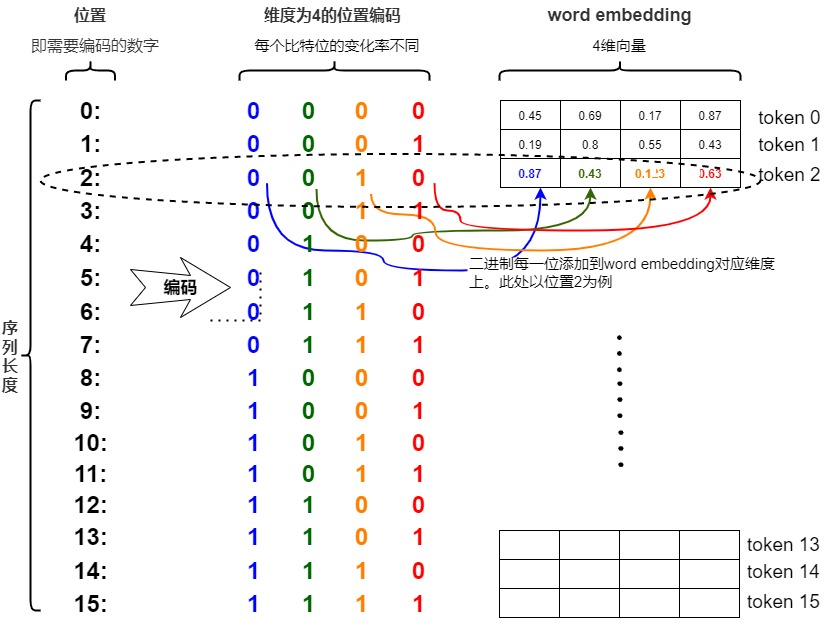
These alternatives are not failed historical trivia. They expose design axes that reappear in relative biases and long-context methods:

Design choice	Identity source	Local relation	Outside training range
scalar integer	magnitude	subtraction	magnitude keeps growing
normalized scalar	fraction of current length	length-dependent stride	coordinate meaning changes with length
binary code	bit pattern	discontinuous at carries	more bits or collisions
learned table	learned row	learned indirectly	no row unless resized/remapped
sinusoidal basis	phase across frequencies	analytic shift transform	formula continues, learned use may not
relative bucket/bias	pairwise offset class	explicit in score	bucket clipping or analytic continuation

The final formula is therefore a design answer, not a decorative convention.

0x01 Why unmasked attention is permutation-equivariant without position

Self-attention can compare every row with every other row. That does not mean it knows row order.

Ignore batch and heads for a moment. Given:

$$X \in \mathbb{R}^{n \times d_{\text{model}}}$$

self-attention computes:

$$Q = XW_Q,\quad K = XW_K,\quad V = XW_V$$ $$A = \text{softmax}\left(\frac{QK^T}{\sqrt{d_k}}\right)$$ $$Y = AV$$

Let $P$ be a permutation matrix that reorders rows. If the input becomes:

$$X' = PX$$

then:

$$Q' = PXW_Q = PQ$$ $$K' = PXW_K = PK$$ $$V' = PXW_V = PV$$

The score matrix is permuted in the same way:

$$Q'K'^T = (PQ)(PK)^T = P QK^T P^T$$

After row-wise softmax:

$$A' = P A P^T$$

and the output is:

$$Y' = A'V' = (PAP^T)(PV) = PAY = PY$$

So, for this unmasked attention operator:

SelfAttn(PX) = P SelfAttn(X)

The layer follows the row permutation. It does not, by itself, assign semantic meaning to row index 0, row index 1, or row index 200.

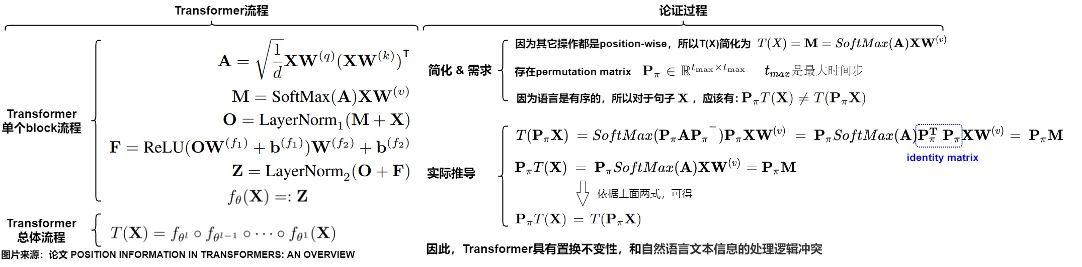
The debugging conclusion for this regime is simple:

unmasked content-only attention follows arbitrary row permutations.
an order-sensitive signal must enter through coordinates, visibility, or another asymmetric structure.

Causal masks and the NoPE boundary

The proof above omitted an attention mask. With an additive visibility mask M, attention is:

$$\operatorname{Attn}_M(X) = \operatorname{softmax}\left( \frac{QK^T}{\sqrt{d_k}} + M \right)V$$

For a causal decoder:

$$M_{ij}= \begin{cases} 0, & j \le i \\ -\infty, & j > i \end{cases}$$

An arbitrary row permutation P does not usually preserve that fixed triangle:

$$PMP^T \ne M$$

Therefore, if the tokens are permuted while the standard causal mask stays tied to row indices, the unmasked proof no longer applies:

$$\operatorname{Attn}_M(PX) \ne P\operatorname{Attn}_M(X) \quad\text{in general}$$

Equivariance can be recovered only if the mask is permuted with the rows:

$$M' = PMP^T$$

but that is not what an ordinary causal language model does. It keeps the lower-triangular mask fixed because row i is allowed to read a prefix ending at i.

This is the opening for NoPE: an autoregressive Transformer can omit an explicit position table or RoPE while still receiving order-dependent structure from causal visibility. Row i has i + 1 visible prefix positions, and deeper layers can compose states produced from progressively different prefix sets. Haviv et al. show empirically that causal language models without explicit positional encodings can learn implicit absolute-position information. Irie later gives a useful qualification: multi-layer autoregressive Transformers can be fully position-sensitive through this cascade, while a one-layer model does not have the same capability at every output position.

The three regimes should not be conflated:

Regime	Explicit PE	Structural order signal	Safe local conclusion
unmasked/bidirectional content-only attention	no	none	arbitrary row permutations are followed equivariantly
causal NoPE attention	no	fixed triangular visibility	order can be inferred from unequal prefix structure
causal or bidirectional attention with PE	yes	coordinates, and possibly a mask	rows receive an explicit coordinate contract

NoPE does not prove that explicit positional mechanisms are useless. Explicit PE, relative bias, and RoPE can provide stronger distance and direction priors, different optimization behavior, and different length-generalization behavior. The precise statement is narrower:

no explicit positional encoding
    does not imply
no order information anywhere in the architecture

---

0x02 Where coordinates can enter

There are several ways to inject coordinate information into a Transformer. M3.3 owns the first three routes and their comparison.

Route	Local form	Owner
causal visibility without explicit PE	fixed lower-triangular mask changes which prefixes each row can read	M3.3 boundary / M3.1 mask mechanics
input-state addition	x_i = content_i + p_i	M3.3
learned absolute table	position_embeddings(position_ids)	M3.3
attention-score bias	scores_ij += b(i,j)	M3.3
Q/K rotation	q_i = rotate(q_i, i), k_j = rotate(k_j, j)	M3.4
length/context extension	coordinate distribution changes beyond training length	M3.5

The distinction matters because all routes can produce working tensors while meaning different things.

Absolute input-level position changes the state row before attention:

X_content:   [B,n,d_model]
coordinate:  [1,n,d_model] or [B,n,d_model]
X_positioned:[B,n,d_model]

Relative position and bias mechanisms work later, at the attention score tensor:

scores: [B,h,q_len,k_len]

RoPE works after Q/K projection and before Q/K dot product:

q, k -> rotate by position -> q_rot, k_rot

M3.3 compares input-state and score paths. M3.4 and M3.5 open rotation and extension.

---

0x02A The immutable positional-call manifest

Shapes are necessary but not sufficient. These two score-bias tensors are both [1,h,1,513]:

correct:
    query is logical position 512
    keys are logical positions 0..512

wrong but shape-compatible:
    query was reset to logical position 0
    keys are still cached positions 0..512

The second call can run without an exception. It answers a different geometric question. A positional mechanism therefore needs an identity contract in addition to a shape contract.

The manifest used by this article is:

positional_call:
    schema: numinens.position-call.v1
    article_owner: M3.3
    public_slug: m3-3-position-encoding-and-context-geometry

    request:
        request_id
        release_id
        checkpoint_id
        adapter_id or none

    row_space:
        storage_rows              # physical order in the packed tensor
        sequence_id_per_row       # which logical example owns each row
        stream_per_row            # encoder / decoder / shared
        logical_position_per_row  # coordinate inside that sequence/stream
        active_token_per_row      # padding is state, not a missing row

    query_space:
        row_indices
        logical_positions
        coordinate_frame

    key_space:
        row_indices or cache slots
        logical_positions
        coordinate_frame

    position_method:
        family                    # fixed_abs / learned_abs / relative / bias / none
        state_object or none
        relation_sign             # key_minus_query / query_minus_key / none
        clipping_or_bucket_rule
        score_bias_shape or none

    visibility:
        mask_id
        polarity
        segment_isolation

    cache:
        cache_id or none
        committed_length
        past_seen_tokens
        coordinate_frame
        checkpoint_id
        release_id

    numerical_state:
        index_dtype
        parameter_dtype
        compute_dtype
        score_accumulation_dtype

    runtime:
        backend_id
        implementation_revision

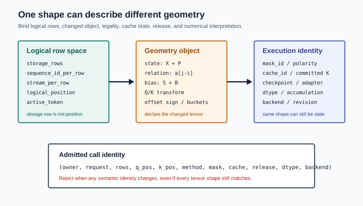
Storage row is not logical position

For an unpacked encoder batch, storage row and logical position are often the same integer. That coincidence disappears under packing:

storage row:       0  1  2  3  4  5
sequence_id:       A  A  A  B  B  B
logical position:  0  1  2  0  1  2

The position table may deliberately reset for sequence B, but the mask must also block A <-> B attention. Resetting coordinates without segment isolation aliases two independent sequences inside one visible score matrix. Conversely, using storage rows 3,4,5 as B’s logical positions silently changes the training distribution even though the packed tensor is valid.

Padding is another policy choice. BERT-style automatic position_ids can stay contiguous across padded storage rows because the padding mask removes those rows from useful attention. A different pipeline may assign a fixed padding position. The manifest records which policy produced the tensor; it does not pretend one numbering rule is universal.

Query and key coordinates are separate ranges

For square training self-attention:

q_positions = [0, 1, ..., S-1]
k_positions = [0, 1, ..., S-1]

During one-token incremental decode after 512 committed tokens:

q_positions = [512]
k_positions = [0, 1, ..., 512]

The relative-offset matrix must be built from those logical coordinates, not from local tensor indices:

$$R_{ij} = k_j - q_i$$

under a key_minus_query convention. A method that declares query_minus_key must negate the same matrix. Neither sign is intrinsically wrong; mixing the paper’s convention with the implementation’s table order is wrong.

The rectangular coordinate compiler is:

def pairwise_offsets(q_positions, k_positions, sign):
    q = q_positions[:, None]  # [Q,1]
    k = k_positions[None, :]  # [1,K]
    if sign == "key_minus_query":
        return k - q          # [Q,K]
    if sign == "query_minus_key":
        return q - k          # [Q,K]
    raise ValueError("relative method requires an explicit sign")

Bias, visibility, and cache identity remain different objects

A positional score bias is finite model preference:

B_position: [1,h,Q,K] or broadcast-compatible

A visibility mask is legality:

M_visible: [B,1,Q,K] or broadcast-compatible

They may be added to the same score tensor, but they are not interchangeable. The manifest stores separate IDs and polarity. A large negative ALiBi penalty does not make a future key legally visible; a zero relative bucket does not override a packed-sequence boundary.

Cache identity is stricter still. Reusing a coordinate or bias object requires agreement on at least:

request and sequence ownership
committed cache length
coordinate frame and offset sign
checkpoint and adapter identity
position-method configuration
dtype and backend interpretation

A cache from a previous release can have the same [B,h,K,d_h] shape and still be invalid because its keys were produced by different weights or position configuration.

Four calls that the same schema must represent

Call	Row/coordinate identity	Geometry object	Critical guard
padded encoder batch	contiguous rows plus active-token mask	fixed or learned [1,S,D] state	padding policy and mask identity
packed causal batch	storage rows plus sequence-local positions	state coordinate and/or score geometry	reset coordinates and isolate segments
incremental decoder	Q=1, K=past+1, absolute logical offset	rectangular bias/relation or transformed Q/K	q_position == committed_length before append
encoder-decoder cross-attention	target query rows, source key rows	often no shared text-distance relation	do not subtract unrelated coordinate frames

This manifest is intentionally broader than one implementation API. Later sections compile it into a sinusoidal slice, a learned table lookup, a Shaw relation tensor, a T5 bucket bias, or an ALiBi penalty. The invariant is that the same logical call cannot acquire a different geometry merely because the backend packed or cached it differently.

---

0x03 Absolute input-level position: x_i + p_i

The simplest state-level coordinate injection is:

$$x_i^{\text{positioned}} = x_i^{\text{content}} + p_i$$

For a batch:

X_positioned[b, i, :] = X_content[b, i, :] + P[i, :]

The position vector must have the same width as the content state:

X_content[b,i,:]: [d_model]
P[i,:]:           [d_model]

so the sum is still:

[d_model]

For the whole batch:

X_content:    [B,n,d_model]
P[:n]:        [1,n,d_model]
X_positioned: [B,n,d_model]

This is why positional encoding appears right after embeddings in the original Transformer-style stack. M2.2 made each row the right width. M3.3 adds a coordinate of the same width.

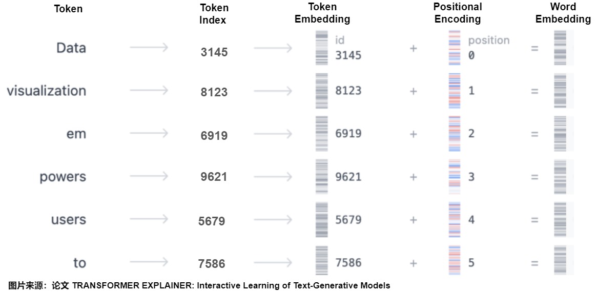
This operation is easy to describe and easy to get wrong. The output shape does not prove the coordinate is right. It only proves a same-width vector was added.

---

0x03A From scalar labels to a multi-frequency coordinate basis

A8’s sequence of integer, normalized, and binary encodings is useful when it is read as a sequence of counterexamples. Each candidate satisfies one design requirement by violating another.

Repeating a raw integer creates a growing rank-one direction

Suppose the scalar position is repeated in every model channel:

$$p_t = \alpha t\mathbf{1}_D$$

Its norm is:

$$\lVert p_t\rVert_2 = |\alpha|t\sqrt{D}$$

If a content row has approximately independent channel scale $\sigma$, then its expected norm is on the order of $\sigma\sqrt{D}$. The ratio is therefore:

$$\frac{\lVert p_t\rVert_2}{\lVert x_t\rVert_2} \approx \frac{|\alpha|t}{\sigma}$$

Width cancels. Increasing d_model does not fix the growing coordinate; the position direction eventually dominates unless later normalization or learned weights compensate. The problem is not that a large index is automatically a large attention weight. It is that the input distribution changes systematically with t along one repeated direction.

Length normalization bounds magnitude by changing coordinate meaning

Normalizing by the current sequence length gives:

$$p_t^{(L)}=\frac{t}{L}\mathbf{1}_D$$

Now the norm is bounded, but the same absolute row changes when L changes:

$$p_2^{(5)}=0.4\mathbf{1}_D, \qquad p_2^{(10)}=0.2\mathbf{1}_D$$

The adjacent-position step also depends on the example:

$$p_{t+1}^{(L)}-p_t^{(L)}=\frac{1}{L}\mathbf{1}_D$$

Thus batching or curriculum changes the coordinate system itself. Normalizing by a fixed declared maximum avoids that particular ambiguity, but then it is just a fixed-scale absolute coordinate with a finite design range, not a sequence-length-invariant solution.

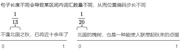
Binary digits are bounded but not locally smooth

With m bits, binary codes distinguish at most $2^m$ integer positions before another bit or a collision policy is needed. Each component is bounded, but consecutive integers do not have a uniform local displacement. At a carry:

7 -> 8
0111 -> 1000

all four bits flip. The Euclidean step is 2, whereas 6 -> 7 changes one bit and has step 1. Binary position is therefore a valid discrete identifier, but it does not supply the smooth multi-scale neighborhood that the construction is seeking.

A symmetric scalar interaction cannot encode signed direction

For scalar or vector coordinates, a symmetric product satisfies:

$$\langle p_m,p_n\rangle=\langle p_n,p_m\rangle$$

so that interaction alone cannot distinguish m - n from n - m. This does not prove that every attention layer using absolute vectors is directionless: different Q and K projections, masks, and content can break symmetry. It proves only that the bare symmetric coordinate inner product cannot represent a signed relation by itself.

One route is a non-commuting or oriented transform, which motivates the RoPE handoff. The route taken here is a bounded continuous basis with many rates of change:

fast channels:
    distinguish nearby positions

slow channels:
    change smoothly over larger spans

paired phases:
    make a fixed offset an analytic linear transform

The first two requirements lead to a geometric ladder of sinusoidal frequencies. The third explains why sine is paired with cosine; 0x06 derives that algebra rather than treating the pair as decoration.

---

0x04 Harvard PositionalEncoding in code

The Harvard Annotated Transformer implementation gives the fixed sinusoidal version as a module:

class PositionalEncoding(nn.Module):
    def __init__(self, d_model, dropout, max_len=5000):
        super(PositionalEncoding, self).__init__()
        self.dropout = nn.Dropout(p=dropout)

        pe = torch.zeros(max_len, d_model)
        position = torch.arange(0, max_len).unsqueeze(1)
        div_term = torch.exp(
            torch.arange(0, d_model, 2) * -(math.log(10000.0) / d_model)
        )
        pe[:, 0::2] = torch.sin(position * div_term)
        pe[:, 1::2] = torch.cos(position * div_term)
        pe = pe.unsqueeze(0)
        self.register_buffer("pe", pe)

    def forward(self, x):
        x = x + self.pe[:, : x.size(1)].requires_grad_(False)
        return self.dropout(x)

This is the main fixed-absolute source object for M3.3.

Code object	Shape / role
x	already [B,n,d_model]
pe = zeros(max_len,d_model)	fixed coordinate table
position	[max_len,1] absolute index column
div_term	[d_model/2] frequency ladder
pe[:, 0::2]	sine values for even dimensions
pe[:, 1::2]	cosine values for odd dimensions
pe.unsqueeze(0)	[1,max_len,d_model] batch-broadcastable table
register_buffer("pe", pe)	non-parameter tensor saved and moved with the module
self.pe[:, :x.size(1)]	[1,n,d_model] slice for current sequence length
x + pe_slice	[B,n,d_model], same shape with coordinate mixed in
dropout(x)	dropout after content and position are summed

The layout assumption is important. This Transformer System execution spine uses batch-first tensors:

x: [B,n,d_model]

so:

x.size(1)

is the sequence length. If an implementation uses:

[n,B,d_model]

then the sequence dimension is axis 0, and this slice is wrong.

The buffer detail matters too. pe is not a learned parameter in this implementation. It is registered as module state so it moves across devices and is saved with the model state, but gradient descent does not train it as a parameter.

This code path also explains the boundary with M2.2:

src_embed = nn.Sequential(
    Embeddings(d_model, src_vocab),
    PositionalEncoding(d_model, dropout),
)

tgt_embed = nn.Sequential(
    Embeddings(d_model, tgt_vocab),
    PositionalEncoding(d_model, dropout),
)

M2.2 owns Embeddings. M3.3 owns PositionalEncoding. Calling only Embeddings(src) and calling src_embed(src) can both produce [B,n,d_model]; only the second includes position in the Harvard path.

A reference compiler with explicit offset and layout

The Harvard path assumes an even d_model, an interleaved layout, and a slice starting at zero. Those are common choices, not properties of sine itself. A reference compiler should expose them:

def sinusoidal_table(
    length,
    d_model,
    *,
    logical_offset=0,
    base=10_000.0,
    layout="interleaved",
    odd_width="error",
    construction_dtype=torch.float32,
    output_dtype=None,
):
    if d_model % 2 and odd_width == "error":
        raise ValueError("paired sine/cosine layout requires even d_model")

    pair_count = (d_model + 1) // 2
    pair_index = torch.arange(pair_count, dtype=construction_dtype)
    inv_frequency = torch.exp(
        -math.log(base) * (2.0 * pair_index / d_model)
    )                                                     # [P]
    position = torch.arange(
        logical_offset,
        logical_offset + length,
        dtype=construction_dtype,
    )[:, None]                                            # [S,1]
    phase = position * inv_frequency[None, :]              # [S,P]

    sine = torch.sin(phase)
    cosine = torch.cos(phase)

    if layout == "interleaved":
        table = torch.empty(length, d_model, dtype=construction_dtype)
        table[:, 0::2] = sine
        table[:, 1::2] = cosine[:, : d_model // 2]
    elif layout == "concatenated":
        # With an odd width, the final channel is the unpaired highest sine.
        table = torch.cat(
            [sine, cosine[:, : d_model // 2]], dim=-1
        )
    else:
        raise ValueError("unknown sinusoidal layout")

    return table if output_dtype is None else table.to(output_dtype)

For even width, the two layouts contain the same paired coordinates under a fixed channel permutation:

interleaved:
    [sin_0, cos_0, sin_1, cos_1, ...]

concatenated:
    [sin_0, sin_1, ..., cos_0, cos_1, ...]

They are not checkpoint-interchangeable unless every downstream weight column is permuted consistently. Shape equality does not make storage conventions equivalent.

For odd width there is no complete final sine/cosine pair. A system should either reject the configuration, as the strict reference does, or document an unpaired tail convention. Standard Transformer widths are usually even, so a silent odd-width workaround is less useful than an explicit policy.

logical_offset is required for chunks and incremental calls. Constructing arange(length) inside a chunk resets its geometry; constructing arange(offset, offset + length) preserves the coordinate frame declared by the positional-call manifest in 0x02A.

The phase should normally be constructed in at least float32 and cast to the model dtype afterward. Computing large integer positions directly in low precision can lose distinguishable indices before sine or cosine is applied. The numerical analysis in 0x06 measures that precision boundary; this constructor only makes the numerical contract visible.

---

0x05 Sinusoidal table: formula, frequencies, and shape

The fixed table uses sine and cosine at multiple frequencies:

$$PE(pos, 2i) = \sin\left( \frac{pos}{10000^{2i / d_{\text{model}}}} \right)$$ $$PE(pos, 2i+1) = \cos\left( \frac{pos}{10000^{2i / d_{\text{model}}}} \right)$$

The code computes the same thing in vectorized form:

position = torch.arange(0, max_len).unsqueeze(1)      # [max_len,1]
div_term = torch.exp(torch.arange(0, d_model, 2) *
                     -(math.log(10000.0) / d_model)) # [d_model/2]

pe[:, 0::2] = torch.sin(position * div_term)
pe[:, 1::2] = torch.cos(position * div_term)

The product:

position * div_term

broadcasts to:

[max_len, d_model/2]

and fills half the dimensions with sine and half with cosine.

For example:

B = 2
n = 5
d_model = 8
max_len = 5000

the objects are:

x:             [2,5,8]
pe buffer:     [1,5000,8]
pe[:, :5]:     [1,5,8]
x + pe[:, :5]:[2,5,8]

The same position table broadcasts over the batch. Position 0 in row 1 and position 0 in row 2 receive the same position vector unless the model deliberately constructs different position_ids.

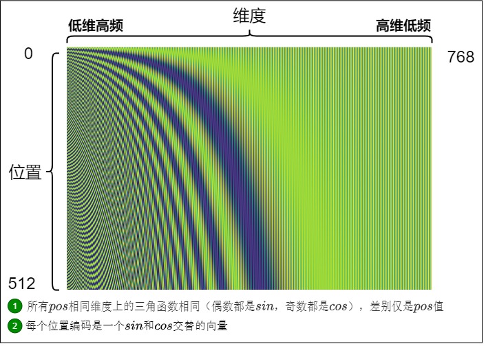
The heatmap shows why this is not just one clock. Different dimensions change at different speeds. Some dimensions vary quickly across adjacent positions; others change slowly and carry longer-wavelength information.

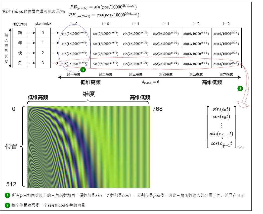
Deriving the frequency ladder and wavelength range

Write one sine/cosine pair with inverse frequency

$$\omega_i = 10000^{-2i/d}, \qquad i=0,\ldots,d/2-1.$$

The angle at position pos is pos * omega_i, and the wavelength measured in token positions is

$$\lambda_i = \frac{2\pi}{\omega_i} = 2\pi\,10000^{2i/d}.$$

This explains the exponent in the implementation. Equal steps in pair index produce equal ratios between wavelengths:

$$\frac{\lambda_{i+1}}{\lambda_i} = 10000^{2/d}.$$

The basis therefore covers scales geometrically rather than spending most dimensions on nearly identical short periods. Pair zero has wavelength approximately 2*pi; the last pair approaches 2*pi*10000 for large d. No one pair uniquely identifies every possible integer position, but the joint phase vector across many incommensurate scales can distinguish a wide operating range and offer both local and coarse variation.

The base 10000 is a hyperparameter, not a theorem that every model must use. Changing the base changes every wavelength except the first. That fact becomes operationally important in M3.4 and M3.5: rope_theta, interpolation, and frequency-band scaling are all changes to the map from (position, pair) to phase.

Boundedness is not uniqueness

Each coordinate component remains in [-1,1], so the position vector norm is bounded. For an even model width with exactly paired sine and cosine channels,

$$\|PE(pos)\|_2^2 = \sum_{i=0}^{d/2-1} \left(\sin^2(pos\omega_i)+\cos^2(pos\omega_i)\right) = \frac{d}{2}.$$

The norm is constant even though direction changes with position. This avoids the scale growth of an integer coordinate, but periodic functions inevitably repeat. The useful claim is not that a finite trigonometric vector is globally collision-free over all integers. It is that the selected multi-frequency basis gives a smooth, bounded coordinate over the intended operating range.

The naive attempts help explain why this design exists:

Attempt	What works	What breaks
integer position	unique index	unbounded scale can dominate content
normalized position	bounded	adjacent stride depends on sequence length
binary position	bounded and compact	nearby positions can flip many bits
sinusoidal table	bounded, smooth, multi-frequency	still only an input-level coordinate

The last caveat is important. Sinusoidal position is a useful coordinate system. It is not the whole theory of relative position.

---

0x06 Why sine and cosine are paired

The sine/cosine pair gives each frequency a two-dimensional coordinate:

[sin(theta), cos(theta)]

If we move by an offset $k$, the angle becomes:

$$\theta_{m+k} = \theta_m + \theta_k$$

The angle-addition identities are:

$$\sin(a+b) = \sin(a)\cos(b) + \cos(a)\sin(b)$$ $$\cos(a+b) = \cos(a)\cos(b) - \sin(a)\sin(b)$$

So the pair for position $m+k$ can be written as a linear transform of the pair for position $m$, with coefficients determined by $k$.

For one frequency pair:

[sin(m), cos(m)] -> [sin(m+k), cos(m+k)]

can be produced by a rotation-like matrix that depends on $k$. This is the local reason the original Transformer paper could hope fixed sinusoidal encodings would help the model infer relative offsets.

There is also a clean dot-product intuition. For one pair:

$$\sin(m)\sin(n) + \cos(m)\cos(n) = \cos(m-n)$$

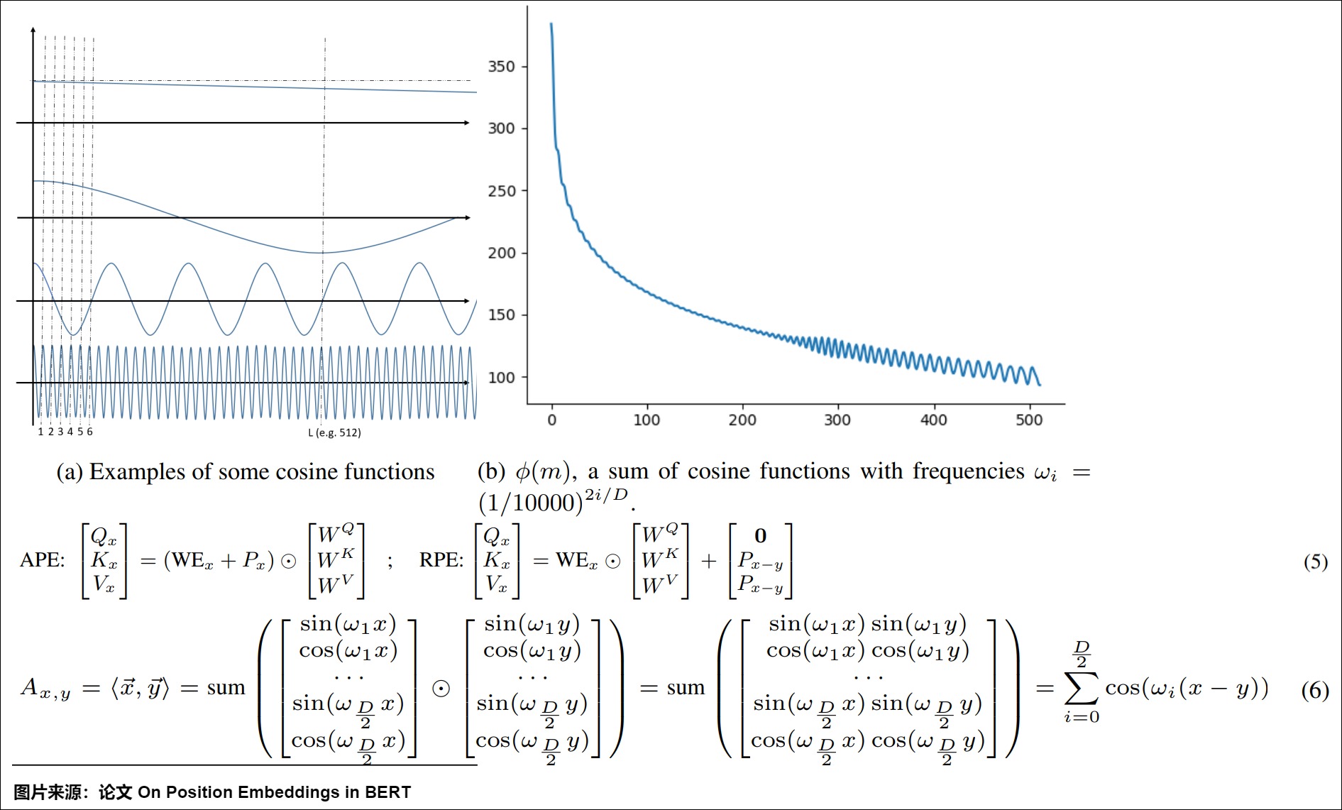
The similarity of pure position vectors depends on the offset $m-n$, not on the two absolute indices separately.

For the whole position vector,

$$PE(m)^TPE(n) = \sum_{i=0}^{d/2-1}\cos\left((m-n)\omega_i\right).$$

That sum is translation invariant: shifting both positions by the same amount does not change it. It is also oscillatory rather than guaranteed monotonic in distance. “Contains relative information” must not be rewritten as “creates a strictly decreasing distance penalty.”

The angle-addition equations yield a stronger implementation statement. Define

$$r_i(m)= \begin{bmatrix} \sin(m\omega_i)\\ \cos(m\omega_i) \end{bmatrix}.$$

Then an offset k can be applied by a fixed 2x2 transform:

$$r_i(m+k) = \begin{bmatrix} \cos(k\omega_i) & \sin(k\omega_i)\\ -\sin(k\omega_i) & \cos(k\omega_i) \end{bmatrix} r_i(m).$$

Stacking these blocks gives one block-diagonal linear map per offset. This is the direct bridge from additive sinusoidal PE to the rotation construction in M3.4.

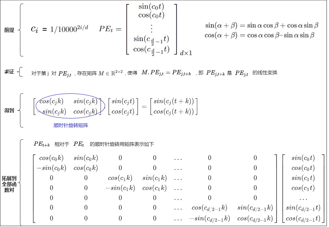
This is useful but limited.

Once the model computes learned projections:

$$Q = XW_Q,\quad K = XW_K$$

the clean positional structure is mixed with token content and learned matrices. The model can learn to use the signal, but input-level sinusoidal PE is not the same thing as explicitly adding a relative-distance term to the attention score.

To see why, expand one attention score. Let

$$q_i=(x_i+p_i)W_Q, \qquad k_j=(x_j+p_j)W_K.$$

Then

$$q_i k_j^T = x_iW_QW_K^Tx_j^T +x_iW_QW_K^Tp_j^T +p_iW_QW_K^Tx_j^T +p_iW_QW_K^Tp_j^T.$$

The four terms are respectively content-content, content-position, position-content, and position-position interactions. The last term would have the clean cos(i-j) structure only under restrictive projection behavior. Arbitrary learned W_Q W_K^T can mix pairs and frequencies, so the pure position dot-product identity does not survive unchanged.

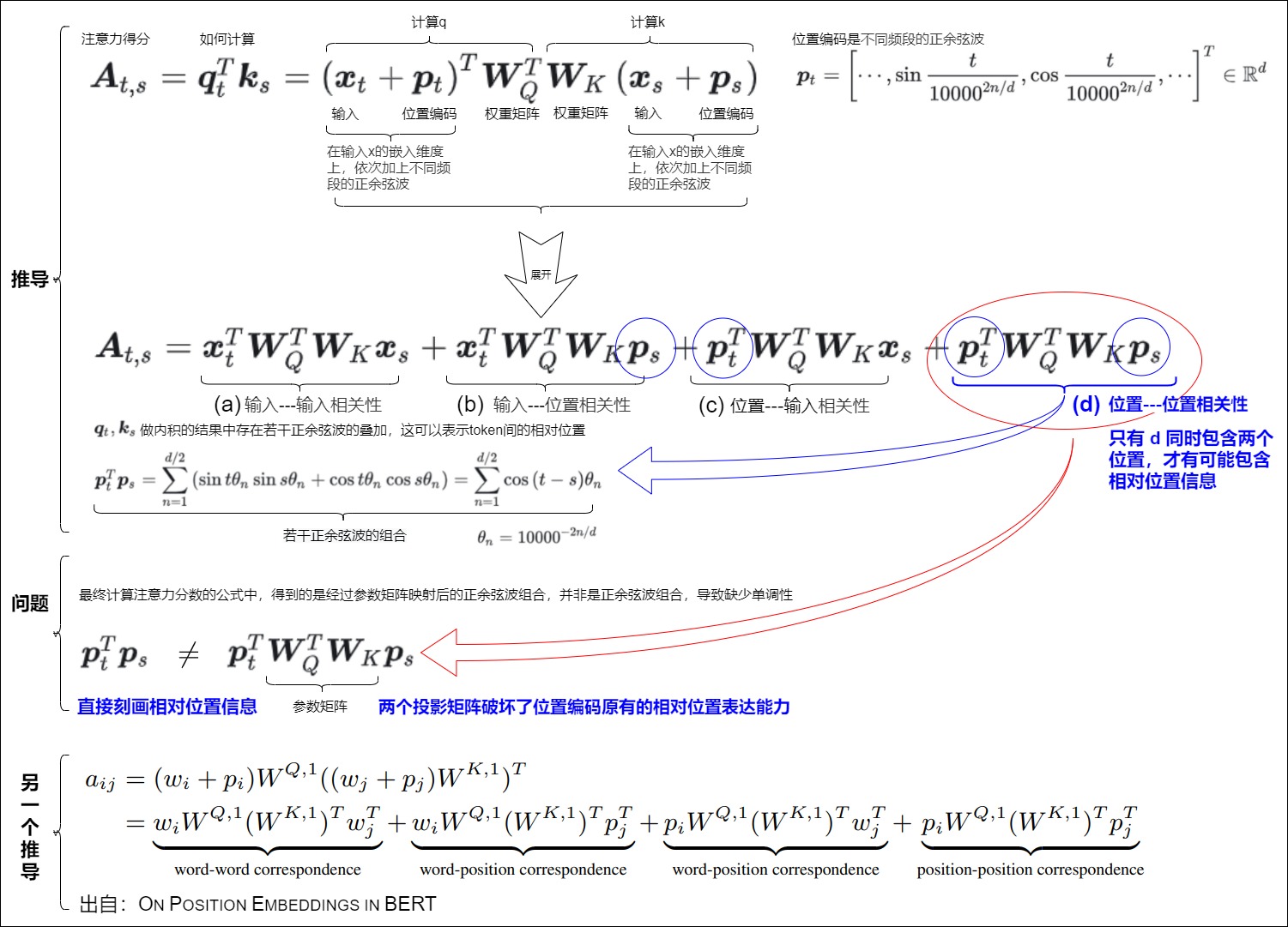
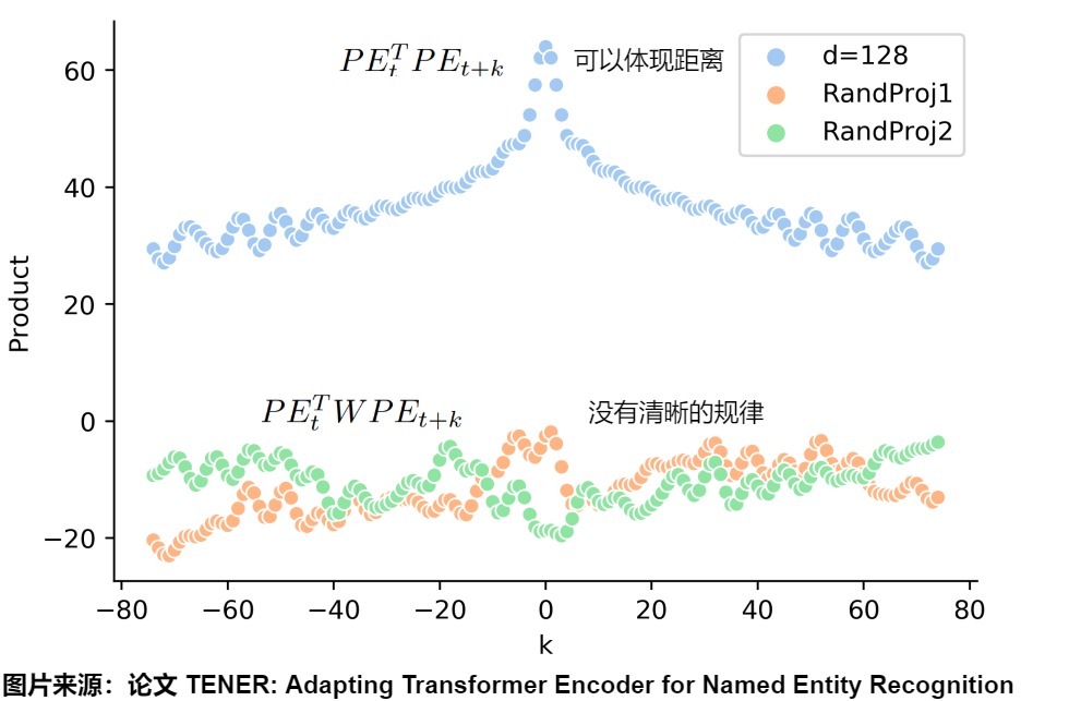
That caveat is the bridge from the absolute-coordinate half of M3.3 to its pairwise score mechanisms.

The shift matrices form a representation of integer translation

For one frequency, define the column convention already used above:

$$r_i(t)= \begin{bmatrix} \sin(t\omega_i)\\ \cos(t\omega_i) \end{bmatrix}, \qquad A_i(k)= \begin{bmatrix} \cos(k\omega_i) & \sin(k\omega_i)\\ -\sin(k\omega_i) & \cos(k\omega_i) \end{bmatrix}.$$

Then:

$$r_i(t+k)=A_i(k)r_i(t).$$

The angle-addition identities also give three structural invariants:

$$A_i(0)=I, \qquad A_i(a)A_i(b)=A_i(a+b), \qquad A_i(k)^{-1}=A_i(k)^T=A_i(-k).$$

So each pair is an orthogonal representation of integer translation. Stacking the pairs produces a block-diagonal matrix $A(k)$ with the same properties:

$$PE(t+k)=A(k)PE(t).$$

This statement is stronger and more precise than saying that nearby positions are “linear.” The offset operation is linear in the coordinate vector; the map from integer t to sine/cosine components is not a linear function of t.

Norm preservation follows immediately:

$$\lVert A(k)PE(t)\rVert_2 = \lVert PE(t)\rVert_2.$$

The group identity is also an implementation oracle: applying offset a and then b must reproduce direct construction at t+a+b. A sign error in one 2x2 block can preserve shape and norm while violating this composition.

Which learned projections preserve joint-shift invariance?

The pure position dot product uses the identity bilinear form:

$$s_{mn}^{\text{pure}}=PE(m)^T I\,PE(n).$$

After position is mixed through learned Q/K maps, the position-position term has a general matrix:

$$s_{mn}^{\text{position}} = PE(m)^T M\,PE(n), \qquad M=W_QW_K^T.$$

Shift both indices by c:

$$s_{m+c,n+c}^{\text{position}} = PE(m)^T A(c)^T M A(c)PE(n).$$

Therefore the score is guaranteed to depend only on relative displacement only if:

$$A(c)^T M A(c)=M \quad\text{for every relevant }c.$$

M = I satisfies this condition. For distinct frequencies, arbitrary cross-frequency mixing generally does not. Within one 2D frequency pair, a matrix of the form:

$$M_i=a_iI+b_iJ, \qquad J= \begin{bmatrix} 0 & 1\\ -1 & 0 \end{bmatrix}$$

commutes with every rotation block. The a_i term contributes a cosine of the offset; the b_i term can contribute an oriented sine term. This shows both possibilities:

learned projections can preserve or learn relative structure,
but arbitrary learned projections are not forced to preserve it.

A cross-frequency matrix entry is a compact counterexample. If one score term multiplies the fast sine channel at m by a slower sine channel at n, then shifting both positions changes both phases at different rates. The offset m-n stayed fixed, but the score can change.

Mathematical coordinates versus finite-precision coordinates

The identities above are real-number statements. A runtime first represents the integer index, constructs phases, evaluates trigonometric functions, and stores the resulting table. Each stage has a dtype.

Binary floating-point formats stop representing every consecutive integer at different thresholds:

Format used for the position scalar	Last power-of-two boundary before the next integer aliases	Example alias
bfloat16	$2^8=256$	256 and 257 round to the same scalar
float16	$2^{11}=2048$	2048 and 2049 round to the same scalar
float32	$2^{24}=16{,}777{,}216$	16,777,216 and 16,777,217 round to the same scalar

If aliasing occurs before multiplying by inverse frequency, every phase and every output channel is identical for those two positions. This is why the reference compiler constructs positions in at least float32 rather than in the model’s float16 activation dtype.

Even when phase construction is distinct, casting the completed table to a lower precision can make two nearby rows numerically difficult to distinguish in slow channels. The relevant runtime question is not only:

Are the mathematical vectors different?

It is also:

At the declared base, width, position range, and storage dtype,
what is the minimum row separation and does any pair collide?

That is a finite-range measurement, not a global uniqueness proof. Periodic components repeat, the joint vector is stored finitely, and a model can ignore distinguishable coordinates. The safe claim is:

sinusoidal PE defines a bounded analytic coordinate for any integer
that the construction can represent;

it does not guarantee globally unique finite-precision rows,
nor useful behavior at lengths absent from training.

Executable algebra checks

The minimal oracle mirrors the derivation:

direct = pe(t + a + b)
composed = A(b) @ (A(a) @ pe(t))
assert_close(direct, composed)

pure_1 = pe(m).T @ pe(n)
pure_2 = pe(m + c).T @ pe(n + c)
assert_close(pure_1, pure_2)

mixed_1 = pe(m).T @ M_cross_frequency @ pe(n)
mixed_2 = pe(m + c).T @ M_cross_frequency @ pe(n + c)
assert not_close(mixed_1, mixed_2)

These checks do not prove model quality. They distinguish an analytic property of the coordinate basis from a learned property of the attention projection.

---

0x07 Learned absolute position embeddings and position_ids

Fixed sinusoidal PE is not the only absolute-position route. Many models use learned absolute position embeddings.

The shape path is the same:

token_embeddings:    [B,n,d_model]
position_embeddings: [B,n,d_model]
sum:                 [B,n,d_model]

but the coordinate object is a learned table. In a real module, the table is created once during initialization, then looked up during the forward pass:

class LearnedAbsolutePosition(nn.Module):
    def __init__(self, max_position_embeddings, d_model):
        super().__init__()
        self.position_embeddings = nn.Embedding(
            max_position_embeddings,
            d_model,
        )

    def forward(self, token_embeddings, position_ids=None):
        batch_size, seq_len, _ = token_embeddings.shape

        if position_ids is None:
            position_ids = torch.arange(
                seq_len,
                device=token_embeddings.device,
            ).unsqueeze(0).expand(batch_size, -1)

        position_vectors = self.position_embeddings(position_ids)

        return token_embeddings + position_vectors

The learned position table is:

P: [max_position_embeddings, d_model]

and lookup gives:

P[position_ids]: [1,n,d_model] or [B,n,d_model]

If position_ids is [1,n], the position vectors broadcast over the batch during addition. If position_ids is [B,n], each batch row can carry its own coordinate convention. This is like token embedding lookup, but the address is position, not vocabulary ID.

BERT-style input construction uses this family of interface. It sums token embeddings, segment/type embeddings, and position embeddings. A typical implementation carries objects like:

self.position_embeddings = nn.Embedding(
    config.max_position_embeddings,
    config.hidden_size,
)

self.register_buffer(
    "position_ids",
    torch.arange(config.max_position_embeddings).expand((1, -1)),
    persistent=False,
)

if position_ids is None:
    position_ids = self.position_ids[
        :,
        past_key_values_length : seq_length + past_key_values_length,
    ]

position_embeddings = self.position_embeddings(position_ids)
embeddings = embeddings + position_embeddings

The local consequences:

Object	Consequence
position_ids	integer coordinates, usually [B,n] or [1,n]
position_embeddings.weight	finite table [max_position_embeddings,d_model]
out-of-range position	hard failure or requires resizing/remapping
new resized rows	rows exist, but learned semantics did not transfer automatically
PAD positions	may still receive position IDs; masks still matter
source and target	can both start at 0 while representing different streams

The biggest difference from fixed sinusoidal PE is the finite learned table. If:

max_position_embeddings = 512

then:

position_id = 800

has no learned row unless the table is extended or the positions are remapped. M3.5 owns the broader length-extrapolation problem. M3.3 only needs the local bug: a learned absolute table has a configured row boundary.

Parameter, gradient, and optimizer ownership

For maximum table length $P_{\max}$ and model width $D$, the table owns:

$$N_{\text{position}}=P_{\max}D$$

parameters. At P_max=512, D=768, that is 393,216 values: about 1.5 MiB in float32 or 0.75 MiB in bfloat16/float16 for weights alone. Training state can be larger because gradients, master weights, and optimizer moments are separate ledgers.

Lookup backward is an indexed row reduction. If:

$$Y_{bsd}=X_{bsd}+P_{I_{bs},d},$$

then:

$$\frac{\partial\mathcal{L}}{\partial P_{r,d}} = \sum_{b,s:\,I_{bs}=r} \frac{\partial\mathcal{L}}{\partial Y_{b,s,d}}.$$

Repeated position IDs accumulate into the same table row. Rows not addressed by the batch receive no lookup contribution. Whether the framework stores that gradient sparsely is a separate implementation choice; a standard dense embedding plus Adam-style optimizer can still allocate dense gradient and two dense moment tensors for the entire [P_max,D] table.

The training length distribution determines row support. If examples have effective lengths $L_e$, the number of examples that can update row r is:

$$c_r=\sum_e \mathbf{1}[L_e>r].$$

c_r usually decreases toward the end of the table. Therefore:

configured row exists
    != row was addressed during training
    != row received useful gradient
    != model learned to use that row at evaluation

A checkpoint can contain 512 position rows while a curriculum rarely presents tokens near 511. Table capacity is not training coverage.

BERT-style build order and persistent state

The common BERT-style input path is not only three lookups. Its ordering is:

word_embeddings(input_ids)
    + token_type_embeddings(token_type_ids)
    + position_embeddings(position_ids)
        -> LayerNorm
        -> dropout
        -> encoder

The position table is a trainable parameter. A generated position_ids range may be a non-persistent buffer: it moves with the module but is reconstructed from configuration rather than stored as a learned checkpoint tensor. These objects have different migration rules:

Object	Learned?	Typical checkpoint role	Migration obligation
position_embeddings.weight	yes	persistent parameter	copy/remap old rows; initialize new rows
position_ids range buffer	no	may be non-persistent	regenerate to the new declared maximum
max_position_embeddings	no	configuration	must agree with table row count and admission checks
optimizer first/second moments	training state	optimizer checkpoint	copy old rows; initialize new rows consistently
live K/V cache	request state	not model checkpoint	invalidate when release/checkpoint position contract changes

Initialization is part of the checkpoint contract. New rows initialized with the model’s normal initializer, copied/interpolated from old rows, or generated from a fixed formula begin with different semantics. None is automatically a length-extension solution.

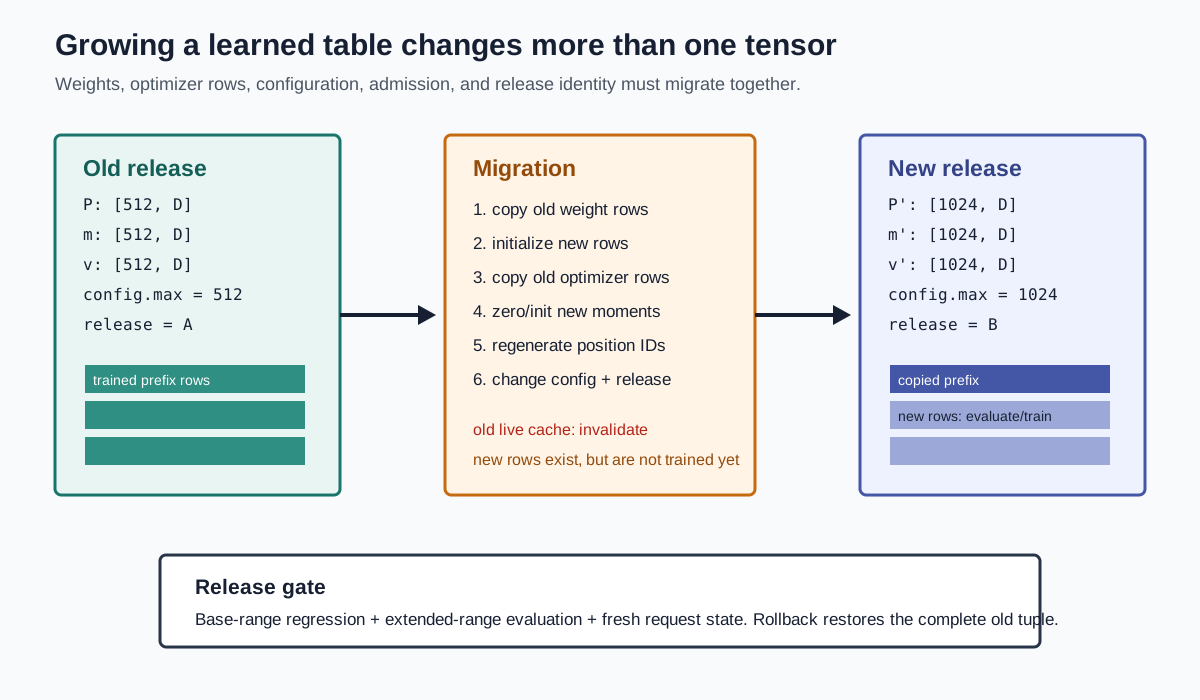
Resizing is a migration, not a configuration edit

To grow from $P_{old}$ to $P_{new}$, define a new parameter:

$$P'\in\mathbb{R}^{P_{new}\times D}.$$

The prefix copy is:

$$P'_{0:P_{old},:}=P_{0:P_{old},:}.$$

Rows P_old:P_new need an explicit initialization policy. A complete migration also changes:

model parameter shape
configuration max_position_embeddings
generated position_ids range
optimizer state shape and row mapping
distributed/sharded checkpoint metadata
release/checkpoint identity
runtime admission limit

The minimal training migration is:

def migrate_position_table(old_weight, old_optimizer, new_rows):
    old_rows, width = old_weight.shape
    new_weight = initialize_position_rows(new_rows, width)
    new_weight[:old_rows] = old_weight

    new_first_moment = zeros_like(new_weight)
    new_second_moment = zeros_like(new_weight)
    new_first_moment[:old_rows] = old_optimizer.first_moment
    new_second_moment[:old_rows] = old_optimizer.second_moment

    return new_weight, new_first_moment, new_second_moment

Copying the old optimizer prefix preserves its accumulated state. New rows usually start with zero moments unless the migration defines another policy. Keeping the old [P_old,D] moments beside a [P_new,D] parameter is not a partial success; the optimizer checkpoint is incompatible.

Release and rollback state machine

Treat the enlarged table as a new release:

DRAFT
    -> TABLE_MIGRATED
    -> OPTIMIZER_MIGRATED          # if training continues
    -> CHECKPOINT_RECONCILED
    -> BASE-RANGE_REGRESSION_PASS
    -> EXTENDED-RANGE_EVALUATED    # owned by M3.5
    -> RELEASED

Admission requires one tuple:

(release_id,
 checkpoint_id,
 position_method,
 table_rows,
 config_max_position_embeddings,
 position_id_policy,
 adapter_id,
 runtime_backend)

A live cache produced by the old release is not reusable under the new tuple, even when head and cache shapes are unchanged. Rollback restores the entire old tuple: old table, old config, old checkpoint, old runtime limit, and fresh request state. It does not shrink only the config while leaving enlarged or retrained weights active.

Migration failure cases

Shape-correct state	Why it is wrong
enlarged weight, old config	new rows exist but callers still reject or never address them
enlarged config, old weight	an admitted ID indexes beyond the parameter
copied weight, stale optimizer moments	the resumed update owns a different row space
initialized new rows labeled “trained”	row existence is confused with gradient support
old cache reused after release change	cached K/V came from a different position/checkpoint contract
base-range regression skipped	extension work can silently damage previously supported positions

The safe local conclusion remains bounded: M3.3 can prove that the migration is internally consistent. M3.5 must still measure whether the new positions work.

---

0x08 Padding, batching, BOS/EOS, and source/target streams

Position IDs must agree with the semantic row, not just the rectangular tensor.

Consider a padded batch:

tokens:
row 0: [<bos>, I, ate, apples, <eos>]
row 1: [<bos>, I, ran, <eos>, <pad>]

A naive absolute position table gives:

position_ids:
row 0: [0, 1, 2, 3, 4]
row 1: [0, 1, 2, 3, 4]

The PAD row still receives a coordinate. That may be fine if every downstream path respects the mask:

attention_mask:
row 0: [1, 1, 1, 1, 1]
row 1: [1, 1, 1, 1, 0]

But if a pooling step, loss path, or debugging path reads row 4 without respecting the mask, the PAD state can leak into the result.

Different models also disagree about how padded positions should be numbered. Some use absolute rectangular positions. Some compress positions over non-PAD tokens. Both conventions can work if the model was trained that way. The bug is mixing conventions.

Special tokens shift positions too. If a chat template inserts:

<bos> <system> ... <user> ...

then every content token after the inserted prefix has a different coordinate. Double BOS, missing BOS, or role markers encoded differently between training and inference can preserve the token IDs and still shift all later positions.

Encoder-decoder models have another boundary: source and target position streams are separate.

src IDs: [B,S]
tgt IDs: [B,T]

src position IDs: [0, 1, 2, ..., S-1]
tgt position IDs: [0, 1, 2, ..., T-1]

Source position 2 and target position 2 are not the same semantic coordinate. They live in different streams. Cross-attention later lets target states read source memory, but it does not mean the two position ID streams are shared.

For example:

source:
    我 吃 了 苹果

target:
    I ate an apple

The source stream uses source order. The target stream uses target order. Cross-attention learns alignment between already-positioned streams.

During inference, padding and position can become serving bugs. Decoder-only batched generation often needs careful left/right padding, last_valid_index, and position bookkeeping. RoPE-style prefill/decode adds cache_position and frequency-slice consistency. M3.4 owns rotary geometry; M3.10 owns request-local last-row, position, and logical frontier alignment; M5.1 owns persistent cache publication/lifecycle, M5.2 scheduling, and M5.3 physical allocation. The M3.3 rule is narrower:

attention_mask, position_ids, and semantic rows must agree.

---

0x08A Training and runtime integration for absolute coordinates

Absolute position is part of the checkpoint and input contract, not a preprocessing decoration. Training must exercise the same coordinate rule that inference will use.

training batch construction:
    choose row order and special-token layout
    construct input_ids and visibility masks
    construct position_ids under the checkpoint convention
    lookup/add coordinate rows
    optimize all downstream layers against that geometry

runtime prefill:
    reproduce the same special-token and position convention
    select exactly the table slice or position IDs for prompt rows

runtime decode:
    continue positions from the accepted prefix
    do not restart after padding, chunk boundaries, or cache reuse

Learned absolute position rows receive gradients according to how often their indices appear. Short-biased training updates early rows far more often than late rows. A configuration may allocate 8k rows while the data mixture rarely updates positions above 2k; allocated capacity and trained coordinate behavior are not equivalent.

def position_coverage(input_batches, max_positions):
    counts = torch.zeros(max_positions, dtype=torch.int64)
    for batch in input_batches:
        visible = batch.position_ids[batch.attention_mask.bool()]
        counts.scatter_add_(0, visible.cpu(), torch.ones_like(visible.cpu()))
    return counts

The coverage histogram belongs beside the length histogram in a training data report. With packed samples, logical position may reset per document, continue through the packed row, or be remapped by a segment-aware method. Each is a different model input even when input_ids are identical.

Checkpoint conversion must also preserve:

position table or deterministic formula
maximum position count
position ID offset and padding convention
whether source and target tables are shared
whether embeddings are added before or after scaling/norm

Changing one item at inference is an architecture change, not a harmless loader option.

0x09 Geometry beyond text: layout, time, event order

Text positions are only one kind of coordinate. X1.1 chooses non-text units and preserves their geometry, while X1.2 projects or resamples their features into language-visible state. M3.3 asks whether coordinate metadata stayed aligned with those rows.

Input type	Coordinate metadata	Boundary
text	sequence index, BOS/EOS offset, padding side	M3.3
source sequence	source positions 0..S-1	M3.3 / M3.2
target sequence	target positions 0..T-1	M3.3 / M3.9
image	patch row/col, flattened patch index, crop/resize mapping	M3.3 geometry; X1 unit choice
document	bbox, page_id, reading_order, line/block/table row/col	M3.3 geometry; X1 unit choice
screenshot/UI	element box, z-order, role/label alignment	M3.3 geometry; X1 unit choice
audio	timestamp, frame index, duration, speaker segment	M3.3 / X1
video	time index plus spatial patch/tubelet coordinate	M3.3 / X1
tool/event	event index, timestamp, parent call ID, dependency edge, status	M3.3 / X1
action	step index, control horizon, coordinate frame	M3.3 / X1

These coordinates do not all become a single 1D sinusoidal table.

An image model may flatten 2D patches into a 1D sequence, use 2D position embeddings, or carry spatial structure inside the vision encoder before projection. A document model may need bounding boxes and reading order. An audio model may need frame time and speaker segments. A tool trace may need parent-call IDs and timestamps.

The invariant is row alignment:

row i in X_positioned
    should still match
coordinate metadata for row i

If rows are sorted, padded, chunked, projected, resampled, or concatenated, the coordinate metadata must follow the same transformation.

This article does not expand those modalities into a second input series. They are listed to make one abstraction explicit: a coordinate can describe a row, a pair of rows, or a structured relation. X1.1 owns non-text unitization and X1.2 owns fusion. M3.3 owns the mathematical distinction.

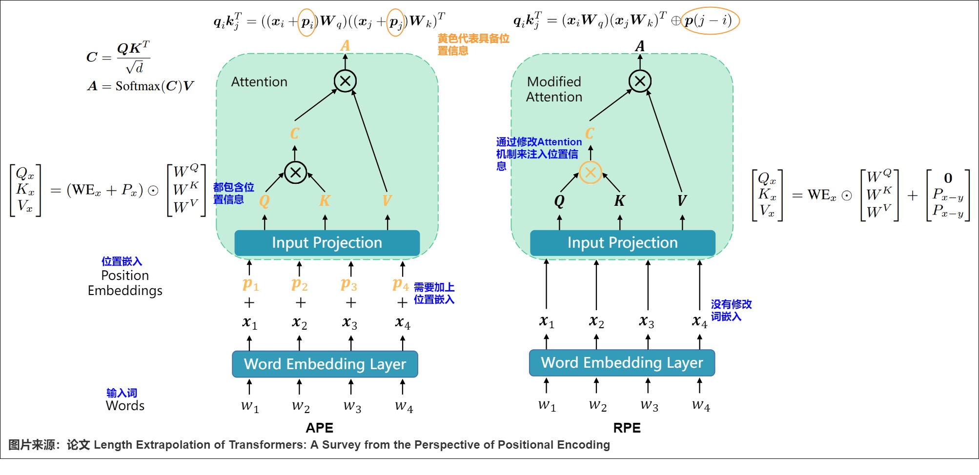
0x09A Pairwise geometry opens the attention score tensor

Absolute position attaches a coordinate to one row. Relative mechanisms attach geometry to a query-key pair. After Q/K projection,

q = project_q(x_q)   # [B,h,q_len,d_head]
k = project_k(x_kv)  # [B,h,k_len,d_head]
v = project_v(x_kv)  # [B,h,k_len,d_head]

content_scores = q @ k.transpose(-2, -1) / math.sqrt(d_head)
# [B,h,q_len,k_len]

The pairwise offset matrix is

$$\Delta_{ij}=j-i$$

under a key-minus-query convention. Some implementations use i-j; the sign is a checkpoint contract. A score-level method builds a broadcast-compatible term and applies it before softmax:

position_term = make_position_term(q_len, k_len, q_start, k_start)
scores = content_scores + position_term
scores = scores.masked_fill(~visibility_mask, -torch.inf)
prob = torch.softmax(scores, dim=-1)
out = prob @ v

Bias and mask have the same shape but different semantics:

finite relative bias:
    preference among legal keys

visibility mask:
    legal versus illegal interaction

A large negative finite bias is not a reliable substitute for a mask. Softmax normalization, dtype limits, and later score transforms can make a supposedly “impossible” route nonzero. Apply the mask as a separate invariant.

Offset construction with unequal query and key ranges

The simple matrix arange(k_len) - arange(q_len) assumes both streams start at global position zero. Cached decoding and segment memory do not.

def relative_offsets(q_len, k_len, q_start=0, k_start=0, device=None):
    q_pos = q_start + torch.arange(q_len, device=device)
    k_pos = k_start + torch.arange(k_len, device=device)
    return k_pos[None, :] - q_pos[:, None]  # [q_len,k_len]

For decode with one new query at absolute position t and keys 0..t:

q_len = 1
k_len = t + 1
q_start = t
k_start = 0
offsets = [-t, ..., -1, 0]

Using local query index zero would instead produce [0,1,...,t], a shape-correct reversal of history.

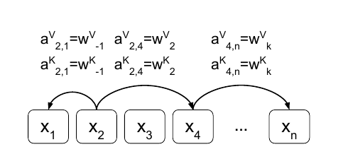
0x09B Shaw-style learned relative key and value vectors

Shaw et al. attach a learned vector to each clipped relative offset. For one head, define

$$a_{ij}^{K}=R^K_{\operatorname{clip}(j-i,-k,k)}, \qquad a_{ij}^{V}=R^V_{\operatorname{clip}(j-i,-k,k)}.$$

The score becomes

$$e_{ij} = \frac{q_i^T(k_j+a_{ij}^{K})}{\sqrt{d_h}} = \frac{q_i^Tk_j + q_i^Ta_{ij}^{K}}{\sqrt{d_h}},$$

and the output is

$$z_i = \sum_j \alpha_{ij}(v_j+a_{ij}^{V}).$$

Deriving the mechanism from labeled attention edges

Ordinary self-attention treats key row j as the same object no matter which query reads it. Relation-aware attention instead treats (i,j) as a labeled edge. For sequential position, its label is the signed displacement. Two learned maps compile that label into key-side and value-side vectors:

edge (query i -> key j)
    -> signed label j - i
    -> clipped class c_ij
    -> key relation a^K_ij
    -> value relation a^V_ij

The key-side vector changes the compatibility calculation. Expanding one dot product gives the two score paths:

$$q_i^T(k_j+a_{ij}^{K}) = \underbrace{q_i^Tk_j}_{\text{content-to-content}} + \underbrace{q_i^Ta_{ij}^{K}}_{\text{content-to-relation}}.$$

The value-side vector changes what is aggregated after softmax:

$$\sum_j\alpha_{ij}(v_j+a_{ij}^{V}) = \underbrace{\sum_j\alpha_{ij}v_j}_{\text{content mixture}} + \underbrace{\sum_j\alpha_{ij}a_{ij}^{V}}_{\text{relation mixture}}.$$

This distinction matters when comparing alternatives. A scalar score bias can change alpha, but it cannot directly add the second relation mixture to the output. Dropping a^V is therefore a real architecture choice, not merely a memory optimization that leaves the same function intact.

Clipping, indexing, and direction

For maximum represented distance k, define:

$$c_{ij}=\max(-k,\min(k,j-i)), \qquad u_{ij}=c_{ij}+k.$$

The signed class c_ij lies in [-k,k]; the physical table row u_ij lies in [0,2k]. Saturation deliberately merges all offsets <= -k into row 0 and all offsets >= k into row 2k.

For a decode query at global position 5, keys at global positions 2..6, and the key-minus-query convention:

key position	raw offset j-i	meaning	clipped at k=2	table row
2	-3	farther past	-2	0
3	-2	past boundary	-2	0
4	-1	recent past	-1	1
5	0	same coordinate	0	2
6	+1	future coordinate	+1	3

The last row may still be illegal under a causal mask. Its relative vector is a finite preference term, not visibility permission. Reversing the subtraction maps past context to positive rows while preserving every tensor shape.

Table ownership and exact tensor contracts

The paper shares relative representations across heads. That gives one key and one value table per owning layer:

R_key:   [2*k+1, d_head]
R_value: [2*k+1, d_head]
index:   [Q,K]

An alternative implementation can learn separate tables per head:

R_key:   [H,2*k+1,d_head]
R_value: [H,2*k+1,d_head]

That multiplies parameter count by H and changes checkpoint layout. If all batch rows share coordinates, index need not carry B. Packed or irregular coordinates can require [B,Q,K], and relation gathers must then preserve the batch/segment identity established by the positional-call manifest.

The tensor trace makes the cost visible:

offset = relative_offsets(q_len, k_len)          # [Q,K]
index = offset.clamp(-max_rel, max_rel) + max_rel

rel_k = rel_key_table(index)                     # [Q,K,Dh]
rel_v = rel_value_table(index)                   # [Q,K,Dh]

content = torch.einsum("bhqd,bhkd->bhqk", q, k)
relative = torch.einsum("bhqd,qkd->bhqk", q, rel_k)
scores = (content + relative) * (d_head ** -0.5)

prob = masked_softmax(scores, visibility_mask)
content_out = torch.einsum("bhqk,bhkd->bhqd", prob, v)
relative_out = torch.einsum("bhqk,qkd->bhqd", prob, rel_v)
out = content_out + relative_out

That code materializes [Q,K,Dh] relation tensors. There are three distinct execution schedules:

Schedule	Key-side temporary	Value-side behavior	Contract
direct gather	[Q,K,Dh]	gather another [Q,K,Dh]	simplest oracle
compact class scores	compute q @ R_key.T as [B,H,Q,2k+1], then gather [Q,K] classes	gather/reduce value rows	avoids key vector expansion
fused tiled kernel	class lookup inside score/output tiles	accumulate relation output inside tile	avoids global relation-vector materialization

The compact schedule is algebraically identical on the key side:

class_score = torch.einsum("bhqd,rd->bhqr", q, rel_key_table.weight)
relative = class_score.gather(
    dim=-1,
    index=index[None, None, :, :].expand(batch, heads, -1, -1),
)

The [B,H,Q,K] score object still exists in ordinary eager attention; what disappears is the extra [Q,K,Dh] key-relation object. A fused attention kernel can tile both, but then its supported relation layout becomes a backend admission condition.

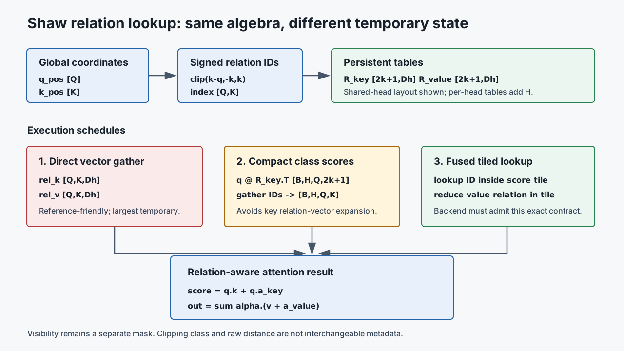
The parameter tables are small:

$$P_{\text{Shaw}} = 2(2k+1)d_h$$

per shared head table, or multiplied by head count if each head owns separate tables. The runtime pairwise object is not small:

$$QK d_h$$

elements if rel_k or rel_v is materialized naively. Efficient kernels avoid or tile that expansion. Parameter count and temporary activation size are different ledgers.

Clipping means every distance beyond k shares an embedding. This controls table size but deliberately removes exact far-distance identity. It is a design choice, not an implementation approximation.

Backward is a reduction by relation class

Let g^e_ij be the gradient of the scaled score e_ij defined above (the softmax input) and g^z_i the gradient of the head output. Because e_ij divides q_i^T a^K_ij by sqrt(d_h), the chain rule leaves one 1/sqrt(d_h) factor in the key-table gradient. For a shared key table row r, lookup backward has the form:

$$\frac{\partial\mathcal L}{\partial R^K_r} = \sum_{b,h,i,j:\,u_{ij}=r} \frac{g^e_{bhij}}{\sqrt{d_h}}q_{bhi}.$$

For the value table:

$$\frac{\partial\mathcal L}{\partial R^V_r} = \sum_{b,h,i,j:\,u_{ij}=r} \alpha_{bhij}g^z_{bhi}.$$

Clipped boundary rows can receive gradients from many raw distances, while interior rows receive only their exact offset. Sharing tables across heads also sums their training signal. A per-head table removes that reduction and changes both statistical support and optimizer state.

Paper variants and design choices

Shaw et al. evaluate more than one switch. The contracts should not be merged:

Variant	Changed object	What remains absent/present
relative key only	score numerator	no relation vector in value aggregation
relative key + value	score and output	full relation-aware formulation
absolute input PE only	input rows	no pairwise relation table
absolute + relative	input and pairwise paths	paper reports no additional translation gain over relative alone in its setup
shared across heads	one table pair per layer	gradients reduce across heads
per-head alternative	one table pair per head	more parameters and a different checkpoint contract

The reported WMT gains and the no-additional-gain result are paper-local experiments, not universal laws. The broader formulation is also not limited to distance: replacing j-i with a typed graph edge yields relation-aware self-attention over graph-labeled inputs. Sequential clipping is one compiler from edge metadata to relation IDs.

0x09C Scalar score biases: T5 buckets and ALiBi slopes

Scalar methods avoid a [Q,K,d_head] relative-vector object. They produce one finite score adjustment per pair and usually per head.

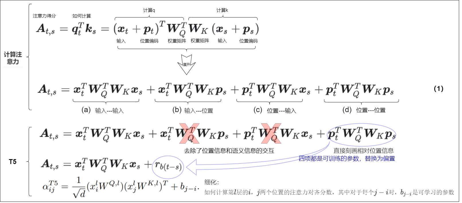
T5: learned buckets with fine local and coarse distant resolution

T5 maps signed relative offsets into a finite number of buckets. Small distances get exact buckets; larger distances are grouped approximately logarithmically until a maximum-distance bucket is reached.

Let B be the total bucket count. In bidirectional attention, each direction receives B/2 buckets. In causal attention, all B buckets describe nonnegative look-back distance after future positions have been removed by the mask. Within one direction, let:

$$B_d= \begin{cases} B/2,&\text{bidirectional},\\ B,&\text{causal}, \end{cases} \qquad E=\left\lfloor\frac{B_d}{2}\right\rfloor.$$

Distances 0..E-1 map exactly. The large-distance branch is chosen by fixing two endpoints in log-distance coordinates:

distance E            -> bucket E
distance max_distance -> bucket B_d (then clamp to B_d-1)

Linear interpolation between those endpoints gives:

$$b_{large}(n) = E+ \left\lfloor \frac{\log(n/E)}{\log(M/E)}(B_d-E) \right\rfloor,$$

then min(b_large, B_d-1). This is why the buckets are exact nearby, progressively wider farther away, and saturated beyond M. The logarithm is not an arbitrary implementation trick; it is the coordinate system in which the far-range bucket boundaries are evenly spaced.

A pedagogical bucket function is:

def relative_position_bucket(relative_position, bidirectional,
                             num_buckets=32, max_distance=128):
    # T5 commonly defines relative_position as memory_position - query_position,
    # then negates it inside the bucketing helper. Preserve the implementation's
    # exact sign convention when converting checkpoints.
    n = -relative_position

    if bidirectional:
        half = num_buckets // 2
        direction = (n < 0).to(torch.long) * half
        n = n.abs()
        num_buckets = half
    else:
        direction = 0
        n = torch.maximum(n, torch.zeros_like(n))

    max_exact = num_buckets // 2
    is_small = n < max_exact
    large = max_exact + (
        torch.log(n.float() / max_exact + 1e-6)
        / math.log(max_distance / max_exact)
        * (num_buckets - max_exact)
    ).to(torch.long)
    large = torch.minimum(large, torch.full_like(large, num_buckets - 1))
    return direction + torch.where(is_small, n, large)

The learned table commonly has shape

relative_attention_bias.weight:
    [num_buckets, num_heads]

and lookup becomes

bucket = relative_position_bucket(offsets, bidirectional=True)  # [Q,K]
bias = table(bucket)                                            # [Q,K,H]
bias = bias.permute(2, 0, 1).unsqueeze(0)                       # [1,H,Q,K]
scores = scores + bias

bidirectional is not a cosmetic flag. Encoder self-attention can represent both past and future directions; causal decoder self-attention normally maps only legal past distances. Cross-attention needs a separately defined geometry because source and target positions do not share one sequence origin by default.

T5 ownership, backward, and stack reuse

For the common table layout [B,H], parameter count is B*H, independent of sequence length. But one must still identify the owning stack and reuse rule. In a common T5 implementation, the first self-attention block in each stack owns the relative-bias table, computes [1,H,Q,K], and later blocks reuse that position-bias tensor. Encoder and decoder self-attention have different bidirectionality; cross-attention does not silently inherit the same table.

If g_bhij is the gradient entering a score bias and bucket(i,j)=r, lookup backward is:

$$\frac{\partial\mathcal L}{\partial W_{r,h}} = \sum_{b,i,j:\,\operatorname{bucket}(i,j)=r}g_{bhij}.$$

If one learned bias tensor is reused in several layers, gradients from every use reduce into the same table. Far saturated buckets aggregate many raw distances, so their training support is not comparable to one exact local bucket.

The reusable runtime object is keyed by more than (Q,K):

(release_id, stack_role, bidirectional,
 num_buckets, max_distance,
 q_start, k_start, Q, K,
 head_count, dtype, device)

Changing bucket count or sign convention changes checkpoint meaning even when the resulting bias tensor still broadcasts.

ALiBi: no table, fixed head-specific linear distance penalty

For a causal head h, ALiBi adds a slope times relative distance:

$$b_{hij}=-m_h(i-j),\qquad j\le i,$$

with positive head-specific slopes m_h. Recent legal keys receive a smaller penalty; distant history receives a more negative one.

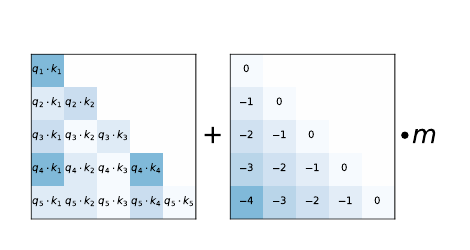
q_pos = q_start + torch.arange(q_len, device=q.device)
k_pos = k_start + torch.arange(k_len, device=q.device)
past_distance = (q_pos[:, None] - k_pos[None, :]).clamp_min(0)

alibi = -slopes[:, None, None] * past_distance[None, :, :]
# [H,Q,K]
scores = scores + alibi.unsqueeze(0)
scores = scores.masked_fill(~causal_and_padding_mask, -torch.inf)

ALiBi’s slopes are deterministic in the paper recipe and differ across heads, creating a range of locality priors. The fact that its formula evaluates at a longer distance supports extrapolation, but does not prove that model behavior or runtime cost remains acceptable at arbitrary length. M3.5 owns that test.

Deriving and assigning ALiBi slopes

For a power-of-two head count H, the paper’s geometric recipe can be written:

$$m_h=2^{-8(h+1)/H}, \qquad h=0,\ldots,H-1.$$

At H=8, this gives:

[2^-1, 2^-2, 2^-3, ..., 2^-8]

Steeper heads encode a stronger recency prior; flatter heads permit relatively more mass at long distance. For a non-power-of-two head count, the reference implementation first generates slopes for the largest lower power of two and then takes alternating slopes from the sequence for twice that power. This is not equivalent to sorting an arbitrary geometric sequence after checkpoint creation: head-to-slope assignment is part of model identity.

def alibi_slopes(heads):
    def power_of_two_slopes(n):
        start = 2 ** (-(2 ** -(math.log2(n) - 3)))
        return [start * start**i for i in range(n)]

    if math.log2(heads).is_integer():
        return power_of_two_slopes(heads)

    lower = 2 ** math.floor(math.log2(heads))
    extra = power_of_two_slopes(2 * lower)[0::2][: heads - lower]
    return power_of_two_slopes(lower) + extra

The paper adds the static bias after the query-key dot product has received its usual 1/sqrt(d_head) scaling. The ALiBi term itself is not divided by sqrt(d_head):

$$s_{hij} = \frac{q_{hi}^Tk_{hj}}{\sqrt{d_h}} -m_h(i-j), \qquad j\le i.$$

Moving the bias inside the scaling changes its effective slope whenever head width changes.

ALiBi runtime state and alternatives

Standard ALiBi slopes are fixed, so no optimizer gradient or learned position checkpoint tensor exists. The runtime still owns slope order, head mapping, coordinate offsets, mask policy, and bias dtype. A decode kernel can generate the distance term from global query/key coordinates or fuse it into score tiles. Reusing a square prefill bias slice for an offset decode query is safe only if its row corresponds to the same global coordinate contract.

Design alternatives must stay labeled:

Choice	Standard paper contract?	Consequence
fixed geometric slopes	yes	no learned position parameters
learned slopes	no	adds optimizer/checkpoint state and can change extrapolation behavior
causal distance penalty	yes for the language-model setup	future visibility still comes from the causal mask
symmetric bidirectional extension	no single canonical paper rule	must define sign/distance and head assignment
input absolute PE plus ALiBi	not the paper’s base method	adds a second positional path

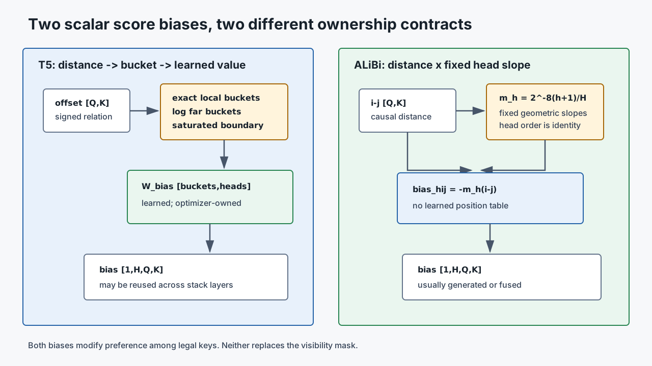
Property	T5 bias	ALiBi
learned position parameters	bucket/head table	none in the standard recipe
local resolution	exact small-distance buckets	linear at every distance
far resolution	logarithmic/coalesced buckets	distinct linear penalty
direction	explicit bucket halves or causal mode	encoded by causal distance/mask
extension behavior	far distances may saturate to last bucket	formula continues linearly
runtime object	[1,H,Q,K] bias	[1,H,Q,K] bias, often generated/fused

0x09D Content-position decompositions: Transformer-XL, DeBERTa, and TUPE

Several paper variants do more than add one scalar distance table. They split content and position interactions so the architecture controls which terms are learned and shared.

Transformer-XL: relative score terms plus segment memory

Transformer-XL caches hidden states from earlier segments and lets current queries attend to the concatenated memory/current keys. Its relative attention score can be organized as

$$A_{ij} = q_i^Tk_j +q_i^Tr_{i-j} +u^Tk_j +v^Tr_{i-j},$$

where r_{i-j} is a projected relative representation and u,v are learned global content and position biases. The four terms are content-content, content-position, global-content, and global-position contributions.

The decomposition is a response to a concrete failure of additive absolute position under segment recurrence. Expanding an absolute-position score would produce:

$$\begin{aligned} (x_i+p_i)^TW_Q^TW_K(x_j+p_j) = {}& x_i^TW_Q^TW_Kx_j \\ &+x_i^TW_Q^TW_Kp_j \\ &+p_i^TW_Q^TW_Kx_j \\ &+p_i^TW_Q^TW_Kp_j. \end{aligned}$$

When cached and current segments both number local rows from zero, p_j is no longer a stable description of their relation. Transformer-XL replaces the query’s absolute-position-dependent terms with two learned per-head biases u,v and replaces key absolute position with a representation of i-j:

$$A_{ij} = \underbrace{q_i^Tk_j}_{AC} +\underbrace{q_i^Tr_{i-j}}_{BD} +\underbrace{u^Tk_j}_{\text{global content}} +\underbrace{v^Tr_{i-j}}_{\text{global position}}.$$

The labels AC and BD match a common implementation split: content-key terms can be multiplied directly, while position terms are computed in a compact relative-coordinate layout and then shifted into query-key alignment.

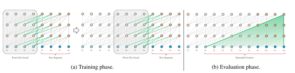
The implementation cannot derive offsets from local tensor indices alone:

memory keys:
    absolute/global positions k_start ... current_start-1

current keys:
    current_start ... current_start+segment_len-1

current queries:
    current_start ... current_start+segment_len-1

The cached memory is normally stop-gradient state between segments. Segment recurrence changes the effective key range and training graph; it is not merely a longer T5 bias matrix.

For current segment tau+1 and layer n, the source-to-tensor contract is:

$$\tilde h_{\tau+1}^{n-1} = [\operatorname{SG}(h_{\tau}^{n-1});h_{\tau+1}^{n-1}],$$

query source:
    current h_(tau+1)^(n-1)              [L,D]

key/value source:
    detached previous h_tau^(n-1)        [M,D]
    concatenated current h_(tau+1)^(n-1) [L,D]
    total                                [M+L,D]

relative rows:
    current query to extended key range  [L,M+L,Dh] conceptually

Memory is layer-indexed. Reusing layer n memory as layer n-1 input is a shape-correct ownership bug. SG also means loss in the current segment does not backpropagate through cached hidden state into the previous segment’s graph. It does not mean the cached rows are numerically zero or excluded from current attention.

Transformer-XL relative shift and decode state

The compact position product is not initially laid out as [query,key]. A relative-shift operation removes a padding column and reinterprets the matrix so each query row reads the i-j representation corresponding to its extended key column. A reference shape trace is:

BD_compact = einsum(q + v, relative_keys)
    [B,H,L,R]

BD_aligned = relative_shift(BD_compact)
    [B,H,L,M+L]

score = (AC + BD_aligned) / sqrt(d_head)

The exact R construction and shift convention belong to the checkpoint and implementation pair. An off-by-one shift often preserves shape while assigning the self-distance row to an adjacent key. A release must therefore pin memory length, segment length, relation-table order, shift function, and u/v ownership together.

DeBERTa: content-to-content, content-to-position, position-to-content

DeBERTa maintains separate content and relative-position representations. A schematic score is

$$A_{ij} = q_i^c(k_j^c)^T +q_i^c(k_{\delta(i,j)}^r)^T +q_{\delta(j,i)}^r(k_j^c)^T.$$

The first term is content-to-content, the second content-to-position, and the third position-to-content. Notice the reversed relative index in the third term. Reusing the same sign for both directional terms is a common silent bug.

For maximum relative distance k, the original clipped relation ID can be written as:

$$\delta(i,j)= \begin{cases} 0,&i-j\le-k,\\ 2k-1,&i-j\ge k,\\ i-j+k,&\text{otherwise}. \end{cases}$$

The position table therefore owns 2k rows, not Shaw’s 2k+1 rows under the earlier convention. The three score tensors are:

content-to-content:  Qc @ Kc.T                         [B,H,Q,K]
content-to-position: Qc dot Kr[delta(i,j)]             [B,H,Q,K]
position-to-content: Kc dot Qr[delta(j,i)]             [B,H,Q,K]

Because the score sums three dot-product paths, the paper normalizes by:

$$\sqrt{3d_h},$$

rather than mechanically retaining sqrt(d_head). Implementations that enable only a subset of position terms must pin their scale-factor rule as part of the architecture contract.

The relative table can own separate position Q/K projections or, in later DeBERTa variants, share projection matrices with content attention. Later variants also add logarithmic position buckets. These are checkpoint-level changes, not harmless optimizations of one fixed equation.

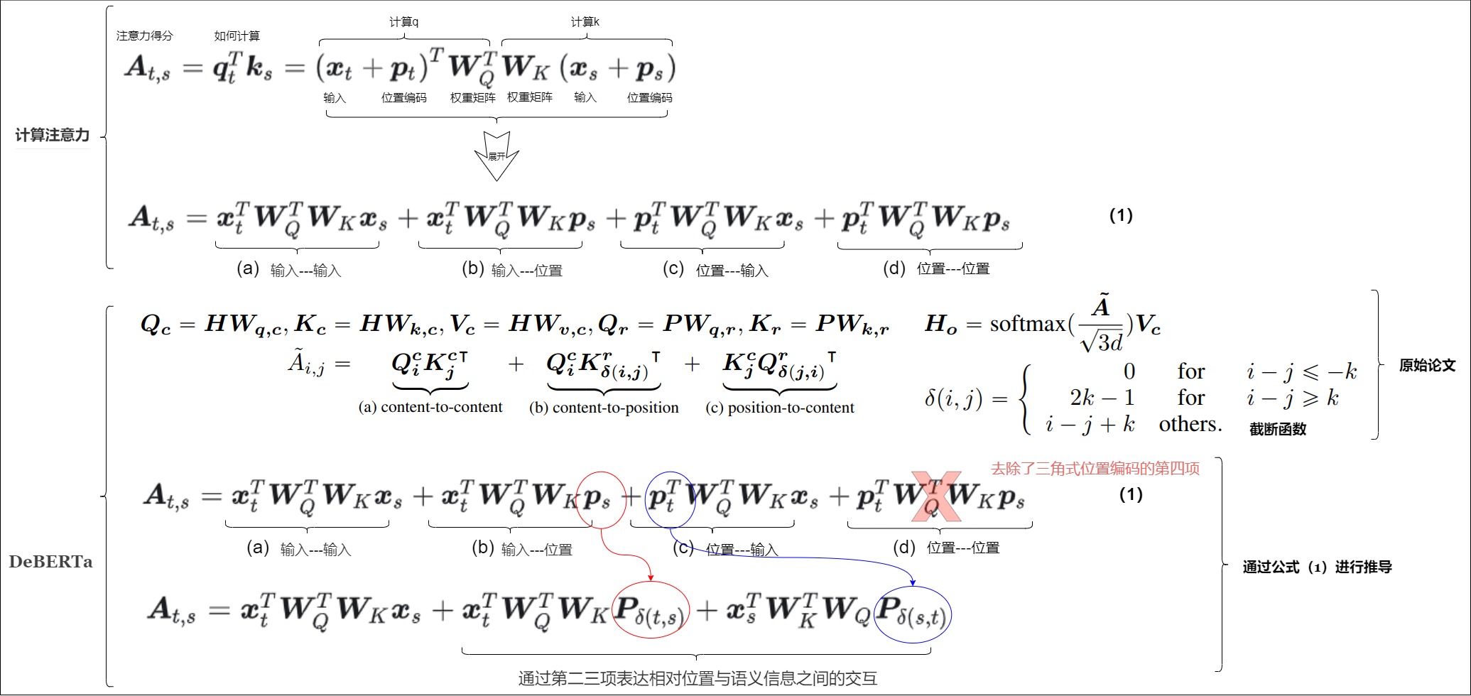
DeBERTa’s enhanced mask decoder is another separate path. The backbone keeps content and relative position disentangled; absolute position is introduced in the masked-token decoding path during pretraining. Describing DeBERTa as simply “BERT plus relative bias” loses both the three-term attention contract and this training-time placement choice.

TUPE: untie content and absolute-position projections

TUPE computes token-content correlation and position correlation through different projections, rather than adding token and position vectors before one shared Q/K projection:

$$A_{ij} = (x_iW_Q^c)(x_jW_K^c)^T +(p_iW_Q^p)(p_jW_K^p)^T.$$

Special treatment can be applied to the [CLS] position because its role is classification aggregation rather than ordinary sequence distance.

The derivation starts from the same four-term additive expansion shown above. TUPE deliberately keeps only independently parameterized content-content and position-position paths:

$$A_{ij} = \frac{ (x_iW_Q^c)(x_jW_K^c)^T +(p_iW_Q^p)(p_jW_K^p)^T }{\sqrt{2d_h}}.$$

The sqrt(2*d_head) denominator records two dot-product contributions. TUPE does not merely assign a new position table while keeping BERT attention unchanged; the content Q/K projections and position Q/K projections are different parameter sets, and the position correlation is built as an explicit per-head score tensor.

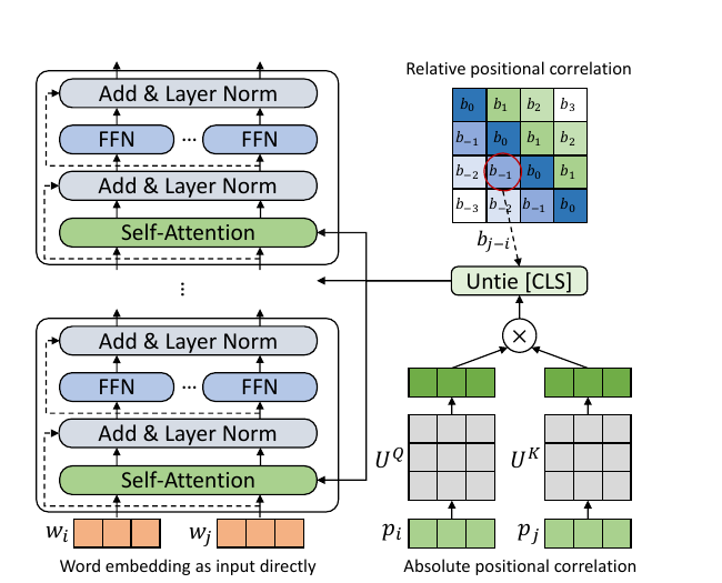
This directly addresses the four-term expansion of additive absolute PE. TUPE keeps the content-content and position-position terms, but avoids forcing the two cross terms to appear through one sum-before-projection operation.

TUPE-A, TUPE-R, CLS, and layer reuse

In the released implementation, a position table has an extra row used to construct special CLS interactions. After position Q/K projection:

ordinary token-token block:
    position_score[:,1:,1:]

CLS query -> ordinary keys:
    replace first score row with a learned per-head CLS-to-other correlation

ordinary queries -> CLS key:
    replace first score column with a learned per-head other-to-CLS correlation

The two directions are not required to be equal. The final position score is computed once, expanded over the batch, and passed as attention bias through the encoder layers in that implementation.

The paper compares two named families:

Variant	Position correlation path	Extra state
TUPE-A	untied absolute position Q/K correlation	learned position table and position projections
TUPE-R	TUPE absolute correlation plus bucketed relative bias in the released code path	relative bucket/head table and special CLS bucket handling

That distinction explains why “TUPE” cannot identify a checkpoint by itself. One must also pin absolute-versus-relative variant, maximum sequence rows, bucket settings, CLS row/column rule, scale factor, and layer reuse.

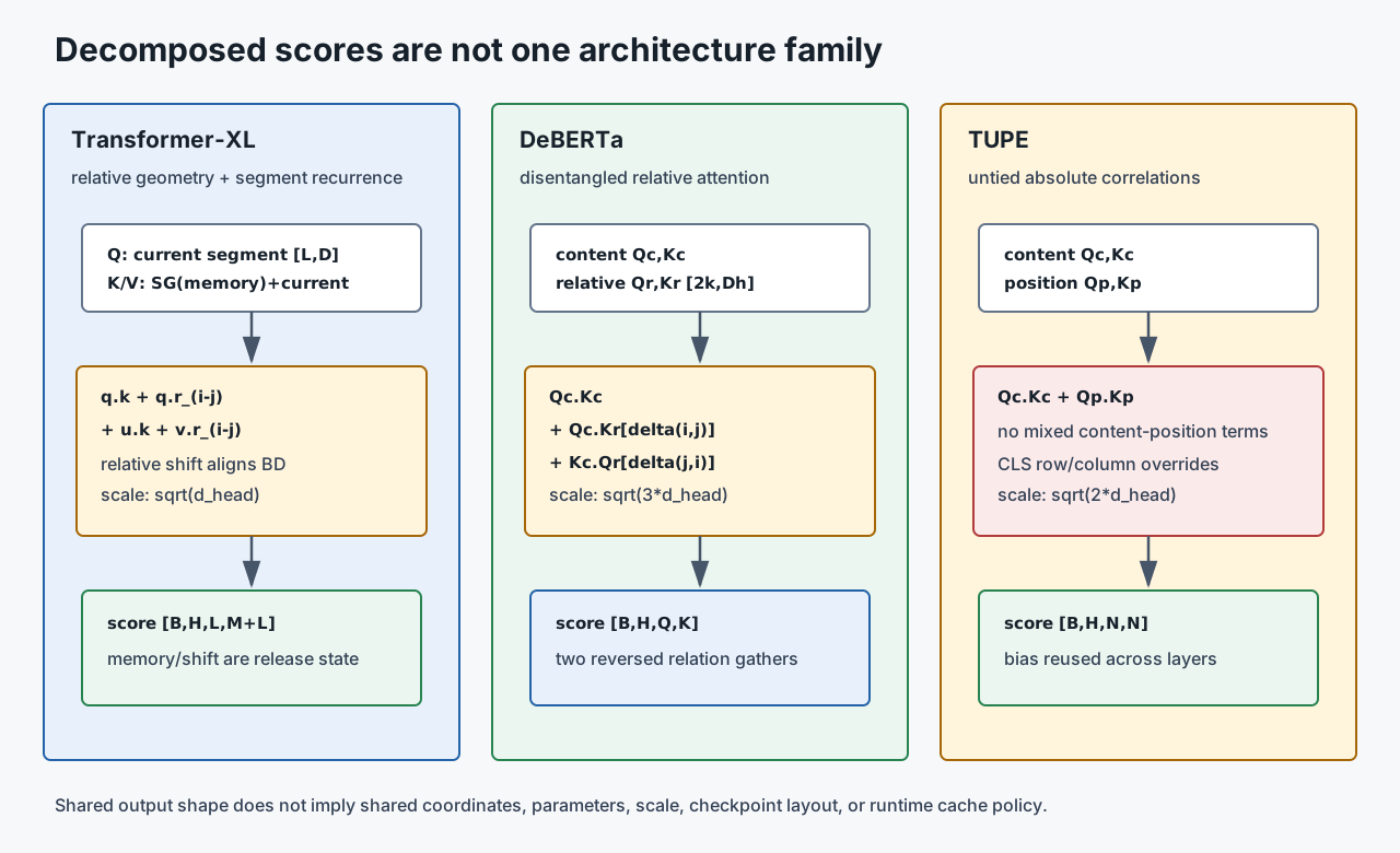
0x09E Method comparison and runtime integration

The paper names are less important than the object each method changes.

Method	State/QK/score object	Learned state	Pairwise temporary work	Cache concern
learned absolute	input state [B,N,D]	[L,D] table	none beyond normal attention	continue position IDs
sinusoidal	input state [B,N,D]	none	none beyond normal attention	continue table/formula indices
Shaw	score and value aggregation	relative K/V tables	potentially [Q,K,Dh]	global offset and clipping
T5	score bias	bucket/head table	[H,Q,K]	bucket correct global offsets
ALiBi	score bias	usually none	[H,Q,K], often fused	use absolute query/key starts
Transformer-XL	score plus recurrent memory	relative projection and biases	extended key range	segment memory ownership
DeBERTa	several score terms	content/position projections	relative index gathers	directional offset conventions
TUPE	separate content/position scores	separate Q/K projections	absolute-position score term	table range and special rows
RoPE	Q/K before score	usually deterministic frequencies	rotation tables, no score-bias matrix	cached K uses same rotation rule

Training-time questions:

Which distances and directions appear in batches?
Are late/far buckets updated often enough?
Does packed training reset or preserve logical coordinates?
Is recurrent memory detached, and how long is it?
Are source, target, and cross-attention geometry modes distinct?

Runtime questions:

Can the kernel fuse the position term, or is a Q*K bias tensor materialized?
Does decode construct offsets from global cache positions?
Are bias tables shared across layers or recomputed per layer?
Does tensor parallelism shard heads consistently with per-head bias state?
Does cache reuse verify the same position scheme and sequence origin?

One robust interface carries coordinates explicitly:

@dataclass
class AttentionGeometry:
    query_positions: torch.Tensor  # [B,Q] or [Q]
    key_positions: torch.Tensor    # [B,K] or [K]
    visibility_mask: torch.Tensor  # broadcastable to [B,H,Q,K]
    mode: str                      # encoder, causal, cross, segment-memory
    scheme_id: str                 # checkpoint/runtime compatibility key

Pinned source-to-runtime trace

Paper equations are not enough to convert or serve a checkpoint. The following official revisions make the implementation claims in this article auditable:

Contract	Pinned official source	Objects that matter
fixed sinusoidal / Harvard composition	Annotated Transformer debc9fd, the_annotated_transformer.py	Embeddings, PositionalEncoding, registered pe, dropout, src_embed / tgt_embed composition
BERT learned absolute	Transformers d09f53a, modeling_bert.py	position_embeddings, non-persistent position_ids, past_key_values_length slice
T5 bucket bias	Transformers d09f53a, modeling_t5.py and T5X 2045b33, layers.py	relative_attention_bias, compute_bias, block-0 ownership, reused position_bias
ALiBi	reference repo 4b92f28	get_slopes, generated alibi, addition to future mask/score path
Transformer-XL	reference repo 44781ed, mem_transformer.py	_rel_shift, r_w_bias, r_r_bias, layer-indexed mems, detached memory update
DeBERTa	official repo 4d7fe0b, disentangled_attention.py	pos_att_type, scale_factor, relative_pos, c2p/p2c gathers
TUPE	official repo 4c64ff7, transformer_sentence_encoder.py	pos_q_linear, pos_k_linear, attn_scale_factor=2, CLS overrides, optional relative table

These pins are evidence snapshots, not a claim that the newest library release must preserve the same API or state-dict path.

Checkpoint conversion must name the changed objects

A converter should begin from a declared source and target contract:

@dataclass(frozen=True)
class PositionCheckpointContract:
    family: str
    source_revision: str
    table_layout: str
    table_rows: int | None
    head_count: int
    head_assignment: tuple[int, ...]
    relative_sign: str
    clipping_or_bucket_rule: str | None
    score_scale_factor: int
    cls_rule: str | None
    layer_sharing: str

Conversion is not successful because load_state_dict(strict=False) returns. It must reconcile:

expected and unexpected checkpoint keys
table orientation: [bucket,head] versus [head,bucket]
shared versus per-layer/per-head ownership
relative sign and clipping endpoint convention
score denominator: sqrt(d), sqrt(2d), sqrt(3d), or dynamic enabled-term count
special CLS rows/buckets
non-persistent generated buffers
tensor-parallel head ordering
runtime cache/release identity

For example, transposing a T5 [bucket,head] table can restore shape in a target implementation that expects [head,bucket]; it does not prove that encoder/decoder ownership, sign, or bucket endpoint semantics match.

Backend admission and fallback

Not every positional family can be expressed through an additive SDPA mask:

Family	Plain additive score-bias path sufficient?	Extra backend contract
learned/sinusoidal input addition	yes, before Q/K/V	position rows must be aligned before projection
T5 / ALiBi	usually for semantics	additive [B/H,Q,K] bias, dtype, offset, and mask composition
Shaw key-only	possible after compact/gather score construction	backend must produce or accept relation score
Shaw key + value	no	relation vector must also enter post-softmax value aggregation
Transformer-XL	no generic drop-in	extended memory K/V, relative shift, and global biases
DeBERTa	no generic single-bias conversion	directional c2p/p2c gathers and term-dependent scaling
TUPE	possible after separate position-score construction	position projections, CLS overrides, and scale remain external

A runtime must either admit a specialized kernel or fall back to an eager reference that preserves the contract. Silently dropping the Shaw value term, one DeBERTa direction, or TUPE CLS override to reach a faster backend changes the model.

def admit_position_backend(contract, backend):
    required = position_capabilities(contract)
    if backend.capabilities.issuperset(required):
        return backend
    if contract.allow_reference_fallback:
        return EAGER_REFERENCE
    raise UnsupportedPositionContract(required - backend.capabilities)

Request state, sharding, and observability

Per-head state follows the same tensor-parallel head partition as Q/K/V:

T5 [bucket,H] table -> shard H consistently
ALiBi [H] slopes    -> shard the same head IDs, preserving order
per-head Shaw table -> shard H; shared Shaw table -> replicate or shared-read
Transformer-XL u/v  -> shard their owning heads
TUPE position score -> shard projected heads before CLS override/reuse

Request and derived-cache identity should include:

(release_id, checkpoint_id, source_revision,
 position_family, variant, sign_rule,
 query_start, key_start, segment_ids,
 table_or_slope_version, head_partition,
 backend_id, dtype)

Useful counters are position_backend, position_fallback_reason, bias_materialized_bytes, relation_materialized_bytes, bucket_min/max, offset_min/max, memory_length, and position_cache_hit. They turn a shape-correct coordinate bug or performance fallback into observable runtime state.

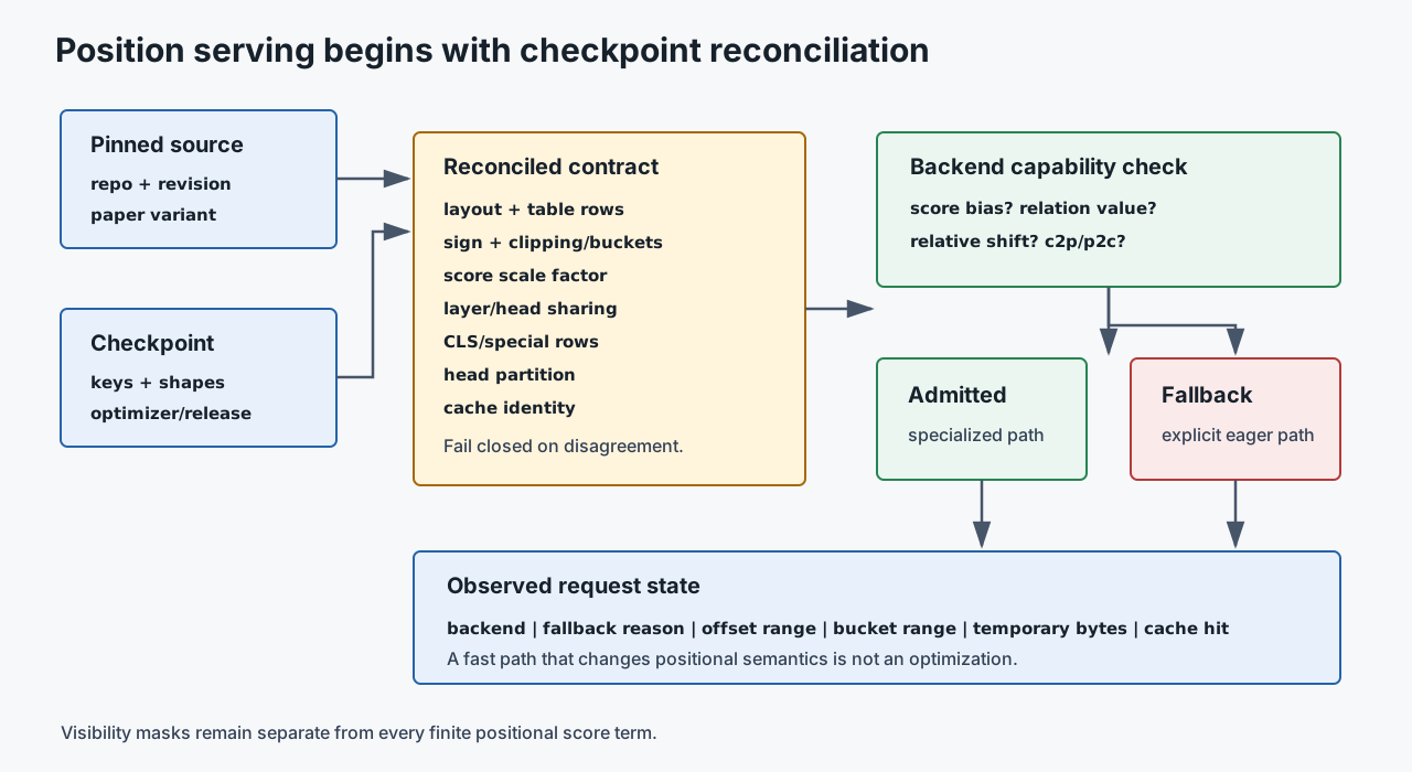
Reconstructing offsets from tensor length is safe only when both sequence origins are known to be zero. Explicit geometry avoids a large class of cached decode and packed-sequence bugs.

---

0x09F Alternative coordinate architectures and the base-regime decision

The mechanisms above are not points on one quality ladder. They change different mathematical objects and break different symmetries. Before selecting a positional family, ask which asymmetry the task supplies naturally and which one the model must learn.

How a causal NoPE stack becomes sequence-sensitive

NoPE means no explicit positional encoding parameter or transform. It does not mean that every row is structurally interchangeable. A fixed causal mask gives row i a nested prefix of i + 1 visible states. The earlier permutation-equivariance proof therefore applies to an unmasked set, not to a causal stack whose visibility triangle stays fixed.

A two-token scalar construction makes the depth qualification concrete. Replace each attention layer by uniform averaging over the visible prefix:

$$y_i^{(\ell)}=\frac{1}{i+1}\sum_{j=0}^{i}y_j^{(\ell-1)}, \qquad y_i^{(0)}=x_i.$$

For the orders [a,b] and [b,a], the last row after one layer is identical:

$$y_1^{(1)}=\frac{a+b}{2}.$$

But the complete first-layer row sets differ:

$$[a,(a+b)/2] \quad\text{versus}\quad [b,(a+b)/2].$$

A second causal layer composes those nested-prefix states:

$$y_1^{(2)}=\frac{3a+b}{4}, \qquad \tilde y_1^{(2)}=\frac{a+3b}{4}.$$

For a != b, the final rows now differ. This is a constructive explanation of how depth plus causal visibility can expose order without an explicit position table. It is not a claim that every optimizer will discover the signal, that a NoPE checkpoint is interchangeable with a PE checkpoint, or that the method will generalize to an unmeasured length. Haviv et al. provide empirical evidence for learned position information; Irie isolates the multi-layer autoregressive qualification.

def uniform_causal_layer(rows):
    out = []
    prefix_sum = 0.0
    for i, row in enumerate(rows):
        prefix_sum += row
        out.append(prefix_sum / (i + 1))
    return out

ab_1 = uniform_causal_layer([a, b])
ba_1 = uniform_causal_layer([b, a])
assert ab_1[-1] == ba_1[-1]
assert uniform_causal_layer(ab_1)[-1] != uniform_causal_layer(ba_1)[-1]

The training and runtime contract is correspondingly strict:

training:
    fixed causal visibility is part of the positional architecture
    depth and boundary-token conventions affect available asymmetry

checkpoint:
    position_family = causal_nope
    there is no table to delete, resize, or silently add

runtime:
    preserve the trained causal mask and row order
    do not substitute a bidirectional/unmasked backend

evaluation:
    measure optimization and length behavior; do not infer them from existence

Deleting learned positions or disabling RoPE in an existing checkpoint does not create a trained NoPE model. It creates a different, generally invalid model.

A flattened index and a 2D coordinate are different priors

Suppose an image-like grid has R rows, C columns, and state width D. A row-major flattening assigns

$$i=rC+c.$$

A full learned table E_flat[i] gives every flattened slot an independent vector and costs

$$N_{\text{flat}}=RCD$$

parameters. It preserves slot identity, but the scalar index alone does not say that (r,c) and (r,c+1) are horizontal neighbors rather than consecutive members of some other traversal.

A separable 2D construction instead uses

$$p_{r,c}=E_{\text{row}}[r]+E_{\text{col}}[c],$$

with

$$N_{\text{separable}}=(R+C)D.$$

It shares every row vector across columns and every column vector across rows. That sharing is an inductive bias and a representational constraint, not merely a parameter optimization. Every 2 x 2 rectangle obeys

$$p_{r_1,c_1}+p_{r_2,c_2} =p_{r_1,c_2}+p_{r_2,c_1}.$$

An arbitrary full R*C table need not satisfy that identity. A richer construction can concatenate row/column features and project them, learn a full 2D table, or add pairwise offsets. Those variants trade sharing, capacity, and runtime state rather than being algebraically equivalent.

def compile_grid_coordinates(row_table, col_table, traversal):
    rows = []
    metadata = []
    for r, c in traversal:
        rows.append(row_table[r] + col_table[c])
        metadata.append({"row": r, "col": c})
    return rows, metadata

If patches are cropped, sorted, dropped, or resampled, traversal and metadata must undergo the same transform as the content rows. Vision Transformer is a useful design counterpoint: it flattens patches and uses learned 1D position embeddings, while still using 2D layout when interpolating those embeddings for a changed image resolution. X1 owns patch construction and projection; M3.3 owns the coordinate identity after those rows exist. Whether an interpolated table works outside its training geometry is an M3.5 evaluation question.

Continuous time needs units, origin, and periodic channels

Event time is not necessarily an integer sequence index. For a timestamp tau, a Time2Vec-style map combines a non-periodic channel with learned periodic channels:

$$\operatorname{t2v}_0(\tau)=\omega_0\tau+\phi_0,$$ $$\operatorname{t2v}_k(\tau)= F(\omega_k\tau+\phi_k),\qquad 1\le k\le K,$$

where the paper uses a periodic activation for the periodic dimensions. This can represent trend and cycles without pretending that event number and elapsed time are the same coordinate.

The source-to-tensor trace must preserve more than a float:

raw event:
    event_id, timestamp, timezone/clock, segment

coordinate normalization:
    tau = (timestamp - declared_origin) / declared_unit

compiled row state:
    content_projection + time_projection(tau)

checkpoint identity:
    origin rule, unit, periodic function, omega/phi layout, missing-time rule

Changing seconds to milliseconds while retaining the same learned frequencies is a shape-correct checkpoint break. Sorting events also requires permuting content, timestamp, masks, and labels together; otherwise the model receives valid tensors describing different events.

Graph structure is not a hidden 1D sequence

A graph has no canonical left-to-right traversal. Graphormer illustrates how the earlier insertion families extend to structural coordinates:

1. Node-level state: add learned in-degree and out-degree vectors to each node feature.
2. Pairwise score bias: map shortest-path distance phi(v_i,v_j) to a learned scalar b_phi.
3. Path relation: add an edge-path term built from features along one selected shortest path.

The score contract is

$$A_{ij} =\frac{(h_iW_Q)(h_jW_K)^T}{\sqrt{d_h}} +b_{\phi(v_i,v_j)}+c_{ij},$$

with the disconnected relation assigned its own ID. The paper’s path term is

$$c_{ij}=\frac{1}{N}\sum_{n=1}^{N}x_{e_n}(w_n^E)^T$$

for a chosen shortest path SP_ij=(e_1,...,e_N). This example matters because it separates a node coordinate, a pair relation, and a path relation in one architecture. Flattening nodes into any arbitrary storage order cannot replace those objects.

A row permutation is valid only if it transports every owned object:

x_prime = x[perm]
degree_prime = degree[perm]
distance_prime = distance[perm][:, perm]
edge_path_prime = edge_path[perm][:, perm]
mask_prime = mask[perm][:, perm]

Permuting only x while retaining the old distance/bias matrix silently attaches structural relations to the wrong node pairs.

Compare contracts, not names

Family	Explicit changed object	Source of asymmetry	Learned positional state	Pairwise work	Base-regime question
unmasked NoPE	none	none	none	none beyond attention	is the task intentionally set-like?
causal NoPE	visibility triangle and depth	nested prefixes	none	causal mask	can training exploit structural order without an explicit prior?
sinusoidal absolute	input row state	fixed coordinate basis	none	none beyond attention	is a deterministic coordinate sufficient?
learned absolute/full grid	input row state	independent slot rows	table and optimizer state	none beyond attention	is fixed support and independent capacity acceptable?
separable multi-axis	input row state	row/column or named axes	per-axis tables	none beyond attention	is additive axis sharing the intended prior?
Shaw relation	score and optionally value path	signed/clipped pair relation	relation-vector tables	relation gather/materialization	should relation content alter scores, values, or both?
T5/ALiBi/graph distance	score bias	bucket, slope, or structural metric	table, fixed slopes, or relation map	scalar [Q,K]/[H,Q,K] term	is a scalar preference expressive enough?
Transformer-XL/DeBERTa/TUPE	decomposed score paths	separate content/position terms	projections, tables, global biases	several positional score terms	which mixed terms and directions should exist?
Q/K transform	projected queries and keys	transform composition	method-specific	transformed Q/K, usually no explicit bias matrix	deferred to M3.4

This table deliberately stops before declaring a winner. Base-regime quality, training stability, kernel support, memory traffic, and train-short/test-long behavior are separate measurements. M3.4 opens Q/K rotation. M3.5 owns extrapolation and context-extension evaluation.

---

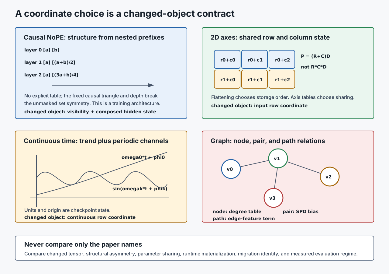
0x0A What M3.3 does not own

M3.3 owns the general positional design space and pairwise score mechanisms. It does not duplicate the complete rotation, extension, kernel, or serving owners.

Later article	Opens which object
M3.4	Q/K rotation, RoPE, freqs_cis, rotate_half, and rotary pairing
M3.5	train-short/test-long, PI, NTK, YaRN, LongRoPE, adaptation and evaluation
M4	whether a kernel fuses coordinate/bias work or materializes it in HBM
M5.1	persistent request/cache schema, publication, committed length, fork/truncate/release, and concurrent-reader lifecycle
M5.2	multi-request admission, scheduling, fairness, and preemption policy
M5.3	physical allocation, mapping, reuse, reference counts, copy-on-write, and deallocation
X1	non-text unitization, multidimensional coordinate ownership, and fusion

The handoff map is:

input-state addition:
    x_i = content_i + p_i
    M3.3

attention-score bias:
    scores_ij = scores_ij + b(i,j)
    M3.3

Q/K rotation:
    q_i, k_j = rotate(q_i,i), rotate(k_j,j)
    M3.4

context extension:
    what happens when coordinate distributions exceed training
    M3.5

This boundary keeps each article inspectable. M3.3 answers both where a row is and how query/key geometry becomes a finite preference. It stops before the specialized RoPE proof and before claims about unseen lengths.

Local storage, addition, and placement ledger

For maximum coordinate length $L_{max}$ and width $d$, a precomputed sinusoidal table and a learned absolute table have the same logical size:

$$N_{\text{position elements}} = L_{max}d.$$

The difference is state ownership. A sinusoidal table is a deterministic buffer; a learned table contains Parameters, gradients during training, and optimizer state. At L_max=8192 and d=4096, one table contains 33,554,432 elements:

bf16/fp16 buffer or weights: 64 MiB
learned parameter count:     33,554,432

Some encoder-decoder implementations instantiate separate source and target position modules, which can duplicate the buffer or parameters. Other models share a rule or compute positions on demand. “Sinusoidal has no parameters” does not mean “sinusoidal has no storage” when the table is precomputed.

Adding positions to a batch performs:

$$B\,n\,d_{\text{model}}$$

scalar additions and returns the same number of state elements. With B=8, n=4096, and d=4096, that is 134,217,728 additions. Absolute input-level position is normally applied once when state rows enter the stack, not once per Transformer layer; multiplying this count by layer depth would describe a different architecture.

Placement is part of the contract. The selected table slice, position_ids, content states, dtype, and device must agree before addition or lookup. Keeping the master table on CPU and copying a long slice every forward can create a transfer bottleneck even though the addition is cheap. Conversely, storing a large table on every pipeline stage duplicates state that may only be consumed at the embedding stage.

---

0x0B Shape ledger

Use this as the M3.3 debugging table.

Object	Shape	Meaning
input_ids	[B,n]	token IDs and aligned sequence metadata from M2.1
X_content	[B,n,d_model]	M2.2 output
position	[max_len,1]	absolute index column
div_term	[d_model/2]	frequency ladder
pe before batch dim	[max_len,d_model]	fixed sinusoidal table
pe buffer	[1,max_len,d_model]	batch-broadcastable buffer
pe[:, :n]	[1,n,d_model]	current position slice
X_content + pe[:, :n]	[B,n,d_model]	positioned state rows
position_ids	[B,n] or [1,n]	learned-position lookup IDs
learned position table P	[max_position_embeddings,d_model]	learned absolute table
P[position_ids]	[1,n,d_model] or [B,n,d_model]	learned coordinate rows
attention_mask	[B,n] or [B,1,1,n]	visibility, not position
query_positions	[Q] or [B,Q]	global/logical query coordinates
key_positions	[K] or [B,K]	global/logical key coordinates
relative_offsets	[Q,K] or [B,Q,K]	signed pairwise displacement
Shaw relative K/V rows	[Q,K,d_head]	learned clipped-offset vectors, if materialized
T5 bucket IDs	[Q,K]	relative-distance classes
scalar position bias	[1,h,Q,K] or broadcast equivalent	finite preference added to scores
Transformer-XL memory	[B,M,d_model] per layer	detached previous-segment state
source states	[B,S,d_model]	source stream after embedding + position
target states	[B,T,d_model]	target stream after embedding + position
layout boxes	[B,n,4] or ragged metadata	document/screenshot geometry
image patch row/col	[B,n,2] or metadata	image geometry
time indices	[B,n]	audio/video/event time
event metadata	ragged or [B,n,...]	event order, timestamp, parent call, status
X_positioned	[B,N_total,d_model]	M3.3 state-route output

The failure pattern:

shape survives.
coordinate contract breaks.

---

0x0C Failure lab

Missing or wrong position addition

Claiming the permutation proof covers a fixed causal mask. The proof in 0x01 is for unmasked attention, or for a mask permuted consistently with the rows. A fixed triangular mask is an order-dependent object.

Treating NoPE as an architecture with no geometry. No explicit position table may be present, but causal visibility still gives different rows different prefix structures.

Removing explicit PE from an existing checkpoint because NoPE can work. NoPE is a training-time architecture contract. Deleting learned or rotary position behavior at inference changes the model function.

Forgetting to add position information.
[B,n,d_model] survives, but reordered rows have no coordinate difference beyond content.

Calling only Embeddings when code expects Embeddings + PositionalEncoding.
Both can return [B,n,d_model]. Only the full src_embed / tgt_embed path includes position in the Harvard stack.

Double-applying positional encoding.
src_embed(src) already adds position, then manual positional_encoding(x) adds it again.

Applying PE before the projector.
H_media: [B,n,d_media] is not necessarily compatible with a [1,n,d_model] table.

Using a PE table built for another d_model.
A fixed table for d_model=512 is not a safe coordinate object for d_model=768.

Shape and layout bugs

Slicing with batch length instead of sequence length.
For batch-first [B,n,d], self.pe[:, :x.size(0)] uses B, not n.

Mixing [seq,batch,d] and [batch,seq,d].
The bug can hide when B and n are accidentally equal or small.

Broadcasting over the wrong axis.
A table shaped for sequence-first code can attach different positions to batch rows.

Forgetting register_buffer.
The fixed table may not move with the module across devices or may not serialize as expected.

Accidentally making fixed PE trainable.
The tensor rank is unchanged, but the implementation no longer matches fixed sinusoidal PE.

position_ids and special-token bugs

Off-by-one positions after BOS or chat-template insertion.
All later content rows shift by one or more positions.

Double BOS/EOS changes coordinates.
This starts upstream in tokenization, but the M3.3 symptom is shifted position IDs.

Source and target streams are confused.
Source position 2 and target position 2 are not the same semantic coordinate.

Decoder prefix positions reset after a prompt.
M3.4 owns RoPE coordinate continuity and M3.10 owns the request-local prefix/frontier transition; the local M3.3 symptom is coordinate reset.

Learned absolute table bugs

Position index out of range.
position_ids.max() >= max_position_embeddings fails or reads invalid coordinates.

Resizing a learned table and assuming semantics transfer.
New rows exist, but they are not trained coordinate semantics.

Using a position table from another checkpoint.
Shape may match while learned coordinate behavior differs.

Interpolating learned positions without checking short-context behavior.
The table now covers more positions, but old positions may behave differently. M3.5 owns the full context-extension problem.

Padding and mask bugs

PAD rows receive position IDs and pooling ignores masks.
Attention may hide PAD, but a later pooling/readout path can still consume PAD states.

Left/right padding changes semantic positions.
Identical prompts can receive different coordinates depending on padding side.

Attention mask and position_ids disagree.
A visible row can get a PAD-like coordinate, or an invisible row can get a content-like coordinate.

Position IDs include PAD columns when code expects compressed non-PAD positions.
Both conventions exist. Mixing them is the bug.

Chunking and multimodal geometry bugs

Long-document chunks reset positions when global order is required.
Each chunk starts at 0, so cross-chunk order disappears.

Long-document chunks preserve global positions when local reset was intended.
Local chunk patterns become harder to learn or debug.

Document geometry detaches from rows.
bbox, page, row, or column metadata no longer refers to the same state row after sorting or batching.

Image patch flattening order changes.
The same patch features use a different row/column convention.

Audio/video timestamps use the wrong stride.
Resampling or frame dropping changes time alignment but metadata is not updated.

Multimodal concat changes row order without moving metadata.
X0: [B,N_total,d_model] is valid, but geometry still points to old row indices.

Tool/event dependency metadata is dropped.
Event rows exist, but parent call, timestamp, or status geometry is gone.

RoPE and cache handoff bugs

RoPE/cache position_ids mismatch.
M3.4 owns the rotary relation, M3.10 owns request-local coordinate/frontier alignment, M5.1 owns persistent cache lifecycle, and M5.3 owns physical allocation or mutation. M3.3 only flags the invariant: token ID, attention mask, position ID, and cache position must describe the same row.

Prefill and decode use different coordinate conventions.
The tensors still line up, but cached keys and new queries can live in incompatible coordinate systems.

Relative-position and score-bias bugs

Using i-j in training and j-i in inference. The relative table or bucket index reverses past and future while every tensor shape remains valid.

Treating a finite position bias as a visibility mask. Illegal future or padding keys retain nonzero probability.

Building decode offsets from local arange(q_len). For q_len=1, the new query is treated as global position zero instead of the current cache position.

Applying a bidirectional T5 bucket mode in a causal decoder. Half the table can encode a direction that should be invisible, and legal past distances use incompatible bucket IDs.

Materializing Shaw relative vectors without a memory ledger. The parameter table is small, but [Q,K,d_head] temporary tensors can dominate activation memory.

Sharing a per-head bias table across a different head order. Tensor parallel repartitioning or checkpoint conversion silently assigns the wrong locality prior to each head.

Reusing a prefix cache across position schemes or origins. Token IDs match, but cached keys were produced with different absolute IDs, RoPE phases, relative offsets, or packed-segment resets.

Calling Transformer-XL memory a normal KV cache. It stores previous hidden states for recurrent segment attention and normally changes the training graph through stop-gradient semantics. The projected serving K/V cache governed persistently by M5.1 and laid out physically by M5.3 is a different object.

Structured-coordinate bugs

Changing grid traversal without recompiling coordinates. The same patch states receive row/column vectors for different cells. A guard must compare traversal identity, crop/resize transform, and coordinate metadata against the content-row manifest.

Changing continuous-time units while reusing learned frequencies. Seconds and milliseconds have the same tensor shape but multiply every learned phase by 1000. Admission must pin origin, unit, periodic function, and missing timestamp policy.

Permuting graph nodes on only one side of a relation matrix. Node rows move, but shortest-path and edge-path entries still name the old ordered pairs. Pairwise state must be transported as R[perm][:,perm].

Failure-to-guard closure

Failure class	Shape can survive?	Mechanical guard	Evidence path
wrong token row / logical coordinate	yes	validate the immutable positional-call manifest and row origin	position-manifest oracle
batch/sequence layout swap	often	assert declared layout and compare slice axis against seq_len	absolute-coordinate oracle
wrong sinusoidal offset, base, or channel layout	yes	compile from frozen fixture and compare interleaved/concatenated conversion	sinusoidal algebra oracle
finite-precision coordinate collision	yes	sweep target dtype and report first indistinguishable positions	sinusoidal precision trace
learned-table row resize without optimizer migration	yes	reconcile weight rows, optimizer rows, config, release ID, and rollback artifact	learned-position oracle
NoPE backend loses causal structure	yes	require causal visibility capability for a causal_nope checkpoint	alternative-coordinate oracle plus backend admission
relative sign reversal	yes	test an asymmetric rectangular (query,key) fixture	Shaw and decomposed-score oracles
finite bias used as mask	yes	validate visibility separately and require illegal-key probability to be zero	scalar-bias oracle
wrong T5 bucket mode or ALiBi head order	yes	freeze bucket IDs, slopes, and tensor-parallel head assignment	scalar-bias oracle
omitted Shaw value or DeBERTa directional term	yes	capability-set admission; reject or use explicit reference fallback	runtime-admission oracle
stale 2D/time/graph metadata	yes	transport row metadata once and pair state on both axes	alternative-coordinate oracle
incompatible checkpoint conversion	yes	fail closed on sign, layout, scale, table rows, sharing, and special rows	runtime-admission oracle
cache reuse across coordinate identities	yes	include position family, origin, offsets, segment IDs, backend, and release in cache identity	positional-call manifest

Every guard above detects a semantic mismatch that ordinary shape checks can miss. The corresponding executable evidence is retained with this article; the publication validator additionally checks local routes, media, source classes, and visual provenance.

---

0x0D Handoff to M3.4

M3.3 exposed two coordinate routes:

absolute state route:
    X_content + coordinate -> X_positioned

relative score route:
    content_scores + pairwise_term -> positioned_scores

The next owner asks whether the relative offset can emerge without adding a separate score-bias tensor. RoPE rotates each Q/K pair by an absolute phase and uses the dot product identity

$$(R_iq_i)^T(R_jk_j)=q_i^TR_{j-i}k_j$$

to make the interaction depend on displacement. M3.4 derives that identity, then follows it through actual tensor layouts, precomputed tables, partial rotary dimensions, cache positions, and implementation variants.

---

0xFF Reference

• Attention Is All You Need
• BERT: Pre-training of Deep Bidirectional Transformers for Language Understanding
• Self-Attention with Relative Position Representations
• Transformer-XL: Attentive Language Models Beyond a Fixed-Length Context
• Exploring the Limits of Transfer Learning with a Unified Text-to-Text Transformer
• Train Short, Test Long: Attention with Linear Biases Enables Input Length Extrapolation
• DeBERTa: Decoding-enhanced BERT with Disentangled Attention
• Rethinking Positional Encoding in Language Pre-training
• Transformer Language Models without Positional Encodings Still Learn Positional Information
• Why Are Positional Encodings Nonessential for Deep Autoregressive Transformers?
• An Image is Worth 16x16 Words: Transformers for Image Recognition at Scale
• Time2Vec: Learning a Vector Representation of Time
• Do Transformers Really Perform Bad for Graph Representation?
• The Annotated Transformer, pinned source revision
• Transformer Series (2) — Overall Architecture
• Transformer Series (7) — Embedding
• Transformer Series (8) — Position Encoding
• Transformer Series (9) — Location Encoding Classification
• Transformer Series (17) — RoPE
• Transformer Series (23) — Length Extrapolation
• Transformer System M1.1 — Architecture and Execution Orientation
• Transformer System X1.2 - Encoders, Projectors, and Fusion
• Transformer System M3.10 — Single-Request Inference Execution
• Transformer System X1.1 - Unitization and Geometry Metadata
• Transformer System M2.2 — Embeddings and Initial Model State
• Transformer System M3.4 — Rotary Position Embedding
• Transformer System M3.5 — Context Extension