M2.1 — Tokenization and Sequence Contracts
M2.1 — Tokenization and Sequence Contracts
0x00 From Text to Token IDs
When we ask a language model to translate a sentence or continue a paragraph, we give it written text. The layers of a Transformer perform calculations on vectors, so we need to decide how that text will be represented before it reaches those layers. One of the first choices is what to represent separately: whole words, parts of words, or smaller units such as individual characters and bytes.
These units are called tokens. A token can correspond to a word, a word fragment, punctuation, or a sequence of bytes. A vocabulary assigns an integer, called a token ID, to each of its entries. The tokenizer is the program that applies the splitting rules and looks up these IDs, turning a sentence into a sequence of integers.
Module 2 follows the conversion from text to vectors in two stages. Tokenization, the subject of this article, produces the IDs. Embedding, explained in M2.2 — Embeddings and Initial Model State, uses each ID to select a learned vector from a table. The ID identifies the piece of text; the selected vector supplies the numbers that the Transformer will work with.
This article is long because it follows both the construction of a tokenizer and its use with a language model. The training texts influence which pieces enter the vocabulary; conversation formats determine which markers are added; and batching determines how several sequences are presented together. We will examine these choices alongside the algorithms that turn text into IDs.
We begin with the training texts and saved tokenizer files, then follow a sentence through encoding, decoding, and batching. Next come the algorithms that learn the vocabulary and split new text. The later sections develop conversation formatting and batching in more detail, then examine vocabulary size, vocabulary updates, and decoding a reply as it is generated. We will also compare models that read bytes or characters directly and work through tests for common errors.
On a first reading, follow the worked examples. The longer derivations and implementation checks can be revisited when you need to implement or debug these steps.
Consider a sentence we want to pass to a Transformer:
The cat sleeps.
We will use the tokenizer released with DeepSeek-V3, so the vocabulary and splitting rules have already been learned. Encoding just the sentence gives:
pieces: ["The", " cat", " sleeps", "."]
IDs:    [671, 7539, 114896, 16]
The first line shows the pieces selected from the sentence; the second shows
their vocabulary IDs in the same order. For example, 7539 identifies
" cat", including its leading space. It will be used to select a vector
from the model’s embedding table. Another tokenizer could choose different
pieces or assign different IDs to these same pieces.
The pieces above are shown as readable text. DeepSeek-V3’s vocabulary uses
Ġ to display a space, so the entry for " cat" is written Ġcat.
The four IDs represent the sentence alone. In a conversation, the model also needs the format used during its training to distinguish a user’s message from an assistant’s reply. For this single user message, the DeepSeek-V3 chat template adds a beginning marker, a user marker, and an assistant marker where the reply will start. These special tokens have their own IDs, so the complete chat input contains seven tokens.
The figure follows this example in two parts. Panel (a) shows how the formatted
message becomes IDs and then vectors. Panel (b) shows how byte-pair encoding
(BPE), the method used by this tokenizer, combines smaller pieces to form
the token " cat". DeepSeek-V3 keeps the capital T and the spaces in
this example.

BOS, User, and Assistant are short labels for DeepSeek-V3’s special
tokens. This example has no system message or earlier conversation, and
ends at the assistant marker, ready for a reply.
In panel (a), an arrow connects each token to its vocabulary ID. The
sequence of IDs is called I. Looking up those rows in the embedding table
E produces X, with one row per input token. The green row shows where
E[7539] goes: it becomes the fourth row of X, after the vectors for
BOS, User, and The. Seven input tokens therefore give seven vectors,
each containing 7,168 values. The drawn cells show the arrangement of the
vectors; they do not show their learned values.
Panel (b) starts with the UTF-8 bytes of " cat", written in hexadecimal:
20 for the space, then 63, 61, and 74 for c, a, and t.
The tokenizer writes the space byte as Ġ. It first merges a with t,
then Ġ with c, and finally Ġc with at. The resulting Ġcat has
ID 7539. The ranks below the merged pieces are positions in the saved
list of merges. When several pairs can be merged, the pair with the smaller rank
is processed first. We will work through this procedure in the BPE section.
The steps and IDs come from the released tokenizer and chat template; the vector size comes from the model configuration.
Learning and Using a Tokenizer
The example assumes that we already have a vocabulary. For methods such as BPE and Unigram, we build it from a collection of training texts, called a corpus. The training algorithm uses patterns in that text to decide which pieces to include and how to split future inputs. This is what training, or fitting, a tokenizer means.
BPE, for example, starts with small units such as characters or bytes. It counts adjacent pairs in the training text, combines the most frequent pair into a larger piece, and repeats. The resulting tokenizer saves its vocabulary, the ID assigned to each piece, and the order in which it learned these merges.
We use this saved information each time we encode a new sentence. The encoder splits that sentence by applying the learned merge priorities; it does not recount pair frequencies or retrain the vocabulary. WordPiece and Unigram learn and apply their vocabularies differently, as we will see later.
The saved files also specify text-processing settings, such as whether to preserve uppercase letters and where splitting is allowed. When we load a tokenizer, we load these settings along with its vocabulary and splitting rules. With a pretrained model, these files are normally supplied alongside the model weights.
The tokenizer and the model must agree on the piece assigned to each ID.
Suppose a tokenizer assigns 7539 to " cat", but the model was trained with
7539 assigned to " dog". The lookup would select the vector trained for
" dog". The ID is within range and the vector has the expected size, so
neither check would expose the mistake. Keeping the original vocabulary and
ID mapping prevents this mismatch.
Pieces, IDs, and Positions
In the sentence alone, " cat" is a piece and 7539 is its ID. It is the second item
in the sequence, at position 1 when counting from zero. If the same piece
appears again, it keeps ID 7539 at a different position. In the formatted
chat input, the two preceding markers move it to position 3. After
embedding lookup, E[7539] is a learned vector. The number 7539 itself
tells us which row to select; its numerical value does not describe the
piece’s meaning.
Some tokenizers first split a sentence into words or other short parts,
often using a regular expression. They then divide each part into vocabulary
pieces separately. If this first step puts The and cat into separate
parts, the next step cannot combine them into one token.
Along with the IDs, a tokenizer can return the start and end positions of
each piece in the original text. These positions are called offsets. For
example, offsets (3, 7) locate " cat" in our sentence, counting characters
from zero and excluding the end position. Some offsets count bytes instead.
The character é, stored as one Unicode code point, takes two bytes in UTF-8;
a displayed character can also combine several code points. We therefore
need to know which unit the tokenizer counts.
Other information can identify inserted markers, such as the beginning of a sequence or the end of a turn. When several examples are placed in a batch, their lengths tell us where each one starts and ends. If text was shortened, we can also record what was removed. This information accompanying the IDs is called metadata.
For a vocabulary with V entries, numbered from 0 to V-1, we can write the
encoding as:
Here, is the input and is its sequence of S token
IDs. specifies the tokenizer and the rules for arranging the
sequence, while holds information such as the offsets and the
length of each example.
The code that prepares the input and the code that runs the model must agree on what the IDs and their accompanying information mean. This agreement is the sequence contract in the title. The model’s saved weights, often called a checkpoint, include an embedding table whose rows must follow the tokenizer’s numbering.
Why Tokenizers Use Different Units
A vocabulary of whole words can represent common sentences with few tokens. But a new word, a misspelling, or an unfamiliar name may have no entry. Smaller pieces let the tokenizer compose such inputs from units it already knows, at the cost of more positions for the model to process.
Learned subword vocabularies include frequent words or fragments as larger pieces and retain smaller units for less familiar text. Character and byte representations use still smaller units; a vocabulary containing all 256 byte values can represent any UTF-8 text, although the resulting sequences may be long. Some of the models examined at the end of this article group bytes into patches before passing them to a larger Transformer.
With a learned vocabulary, our choice of training texts also affects which pieces are available. Let’s look at how those texts are prepared.
0x00A Preparing the training corpus
Suppose we collect web pages to train a tokenizer. A page may contain the article we want, menus, advertisements, and a footer repeated across the whole website. We first extract the text we want to keep. We may also have collected the same page several times.
These repetitions affect the vocabulary we learn. If a page containing
The cat sleeps. appears ten times, BPE counts its pairs ten times. Keeping
one copy changes those counts and may change which pairs are merged first.
Changing the text matters too: converting uppercase letters to lowercase
makes Cat and cat the same string.
The figure follows our repeated page through preparation in panel (a). Panels (b) and (c) then show two different operations: learning a tokenizer from the training texts, and using it to encode documents.

In panel (a), extraction removes the menu and footer from the example page. Deduplication reduces its ten copies to one. Other checks identify each page’s language and format, reject unusable or harmful text, remove sensitive passages, or find material copied from evaluation data. The language labels matter for the tokenizer: the share of each language in the training texts changes which scripts receive short pieces and which are split into many tokens.
We then set aside validation and test documents. They let us check how the
tokenizer handles texts whose words and frequencies did not help choose
the vocabulary. The training documents alone supply panel (b). We choose
which sources to sample and use those texts to learn a tokenizer, called
T in the figure. This is where their word and pair frequencies matter.
Panel (c) uses that same T for all three sets. It applies the saved rules
to each document and returns its IDs; it does not learn a new vocabulary
for validation or test data. Each drawn row represents a separate encoded
document. Combining documents into longer model inputs comes later. In
pseudocode:
tokenizer.fit(train_documents)

train_ids = tokenizer.encode_many(train_documents)
valid_ids = tokenizer.encode_many(valid_documents)  # transform only
test_ids = tokenizer.encode_many(test_documents)    # transform only
For a pretrained model, we skip the learning step in panel (b). We load the
tokenizer supplied with the model and use it as T in panel (c).
Mixing data sources
A corpus can contain books, web pages, code, and several languages. We choose how often to sample a document from each source. In panel (b), this choice determines which texts are used to learn the tokenizer.
Suppose half our sampled documents come from one source and half from another.
After tokenization, their documents average 200 and 800 tokens respectively.
The first source supplies about 200 / (200 + 800) = 20% of the tokens,
despite supplying half the documents.
More generally, let q_s be the probability of choosing source s, and
E[n_s] the average number of tokens in a document sampled from it. The
fraction of tokens we expect that source to supply is:
The denominator adds the contributions from every source. Removing long documents or changing the tokenizer can change these proportions. Counting both documents and tokens tells us how much each source contributes.
Removing unwanted text and repeated documents
Some collected pages contain broken text or almost nothing except menus and advertisements. Filters identify these pages using rules or a model that scores their content. A sample of rejected pages helps us check whether the filter also removes useful code, dialects, or unfamiliar subjects.
To find repeated copies, we can calculate a hash from each document’s text. Identical text produces the same hash. This is called exact deduplication. The following function applies our chosen cleanup rules before calculating the hash:
def exact_dedup_key(document):
    canonical = canonicalize_for_dedup(document)
    return hashlib.sha256(canonical.encode("utf-8")).digest()
Here, canonicalize_for_dedup prepares text for comparison. For example, it
might remove a website’s navigation menu. We can still use a different
version of the text for training. Removing too much during comparison can
make different documents look identical.
Edited copies need a different comparison. One method breaks each document
into overlapping groups of words, called shingles. Using two words per
group, The cat sleeps. gives The cat and cat sleeps.. The sentence
The cat wakes. gives The cat and cat wakes.. There is one group in
common and three distinct groups in total, giving a similarity of 1/3.
This is Jaccard similarity. For two sets of shingles, A and B:
For a large corpus, MinHash estimates this score from a smaller representation of each document. Locality-sensitive hashing (LSH) helps select likely matches without comparing every pair of documents. Embeddings can also find similar passages, although passages about the same subject need not be copies of each other.
The size of the groups, the cleanup rules, and the similarity score required for a match determine which documents are removed. Once we find several copies, we also choose which to keep, taking account of text quality and permission to reuse it.
Other checks look for sensitive information, such as personal contact details, or for test questions and answers that have appeared in the training data. The latter is called benchmark decontamination. Exact matching can miss a translated or paraphrased answer, including one copied into a longer page or generated by another model. Common phrases can produce false matches, and privacy checks can remove unrelated text. Because both kinds of error are possible, we record which method was used and which version of each evaluation set was checked.
Keeping documents separate
If one document ends in rain and the next starts with bow, joining them
without a separator gives rainbow.
The tokenizer may then encode a word that appeared in neither document.
Encoding each document separately avoids this problem.
We can later put several encoded documents into one training sequence to
use the available space. This is called packing. Writing <EOS> for an
end-of-sequence token, two short documents might appear as:
The cat sleeps. <EOS> A train arrives. <EOS>
The inserted token marks the end of a document. The model can still use the first document while processing the second. To prevent this, an attention mask can exclude tokens from the other document, or the attention code can limit its calculation to each document’s start and end positions. Restarting the position count at zero is not enough on its own. For successive passages from one continuous text, using the earlier passage may be intentional.
This pseudocode saves the IDs, the document’s source, and the encoding
settings. The boundary_policy field tells the batching code how to handle
the document when combining it with others:
def encode_document(doc, tokenizer, policy):
    ids = tokenizer.encode(doc.text, bos=policy.bos, eos=policy.eos)
    return EncodedDocument(
        ids=ids,
        source_id=doc.source_id,
        document_id=doc.document_id,
        tokenizer_hash=tokenizer.fingerprint,
        boundary_policy=policy.name,
    )
Preparing conversations
Training texts can also be conversations. Alongside each message, the input must indicate who is speaking: the user, the assistant, or a tool. It may also include instructions and descriptions of the available tools and their arguments. A template specifies how to arrange these parts and which headers or separators to insert.
These additions take up tokens too. The full count includes the formatting as well as the messages:
Here, n_template counts the inserted formatting; the other terms count
system, user, assistant, and tool content. We count after encoding the whole
input, assigning each token to one part only.
A tool description can be longer than the exchange itself, while special IDs for speaker roles can shorten headers if the model was trained to use them. If we train the tokenizer on formatted conversations, repeated headers also affect its vocabulary. To measure lengths and source proportions, we use the complete examples that the model will receive.
Saving the tokenizer with the data
Once the documents have been encoded, we need to know which tokenizer
produced their IDs. The encoded data and the trained model must use the
same tokenizer and conversation format. Otherwise, we can get the cat
and dog mismatch shown earlier.
We save the files along with a description of the training texts and how they were prepared. For each encoded file, the description records:
source and document IDs, with each document's license or provenance class
hash of each document's text before and after cleanup
split: training, validation, or test
versions of the extraction, filtering, deduplication, and privacy steps
decontamination method and the version of each evaluation set checked
tokenizer hash and conversation-template version
encoded length, whether the document was truncated, and its packed position
With this record we can rebuild the encoded data and check it against the model trained on it. The license or provenance class also tells us which documents we may use for training. Even document order can matter: some BPE implementations use it to choose which of two equally frequent pairs to merge first.
Filenames alone are insufficient because a file can change without being renamed. Hashes identify the saved contents. A few short example sentences, saved with their expected pieces, IDs, and decoded text, let us check that loading the tokenizer again gives the same results. The IDs must still select the intended rows in the embedding table and in the model’s output table, if it has one.
For a pretrained tokenizer, we save the exact version selected, even if its original training texts are unavailable.
We can now look inside a tokenizer and see how it stores its vocabulary and the rules used to turn new text into IDs.
0x01 What a tokenizer stores
A saved BPE tokenizer contains a vocabulary with assigned IDs and priorities for merging pieces. To encode the same text again, we also need the rules that split the text before BPE and handle special tokens.
The original Llama 3 implementation provides a short example of how these parts fit together. We will read its constructor in three consecutive excerpts. This example loads Llama’s own vocabulary and uses its own special tokens; the IDs in the opening figure belong to DeepSeek-V3.
Loading the BPE vocabulary
class Tokenizer:
    special_tokens: Dict[str, int]
    num_reserved_special_tokens = 256

    pat_str = (
        r"(?i:'s|'t|'re|'ve|'m|'ll|'d)|"
        r"[^\r\n\p{L}\p{N}]?\p{L}+|"
        r"\p{N}{1,3}|"
        r" ?[^\s\p{L}\p{N}]+[\r\n]*|"
        r"\s*[\r\n]+|"
        r"\s+(?!\S)|"
        r"\s+"
    )

    def __init__(self, model_path: str):
        mergeable_ranks = load_tiktoken_bpe(model_path)
        num_base_tokens = len(mergeable_ranks)
model_path points to the saved BPE vocabulary. The loader returns a
dictionary, mergeable_ranks, whose keys are byte sequences. In tiktoken,
the integer assigned to each entry serves as both its token ID and its
priority during BPE merging: a smaller rank takes precedence. DeepSeek-V3’s
tokenizer.json, shown earlier, stores vocabulary IDs and the ordered list
of merges separately: the merge that produces " cat" has rank 7280,
while the resulting piece has ID 7539.
num_base_tokens counts the entries in this dictionary. These can represent
single bytes, word fragments, whole words, or punctuation.
The regular expression pat_str splits text into smaller spans before BPE
runs. For “The cat sleeps.”, it gives ['The', ' cat', ' sleeps', '.'],
including the spaces before cat and sleeps. BPE then processes each span
separately. We will examine this expression in the next section.
Assigning special-token IDs
The constructor continues by defining special tokens. Some mark the start or end of a text; others delimit message headers or mark the end of a conversation turn. The list also includes unused names reserved for later use:
        special_tokens = [
            "<|begin_of_text|>",
            "<|end_of_text|>",
            "<|reserved_special_token_0|>",
            "<|reserved_special_token_1|>",
            "<|reserved_special_token_2|>",
            "<|reserved_special_token_3|>",
            "<|start_header_id|>",
            "<|end_header_id|>",
            "<|reserved_special_token_4|>",
            "<|eot_id|>",
        ] + [
            f"<|reserved_special_token_{i}|>"
            for i in range(5, self.num_reserved_special_tokens - 5)
        ]

        self.special_tokens = {
            token: num_base_tokens + i
            for i, token in enumerate(special_tokens)
        }
These 256 entries receive IDs immediately after the ordinary vocabulary.
<|begin_of_text|> receives num_base_tokens, <|end_of_text|> receives
num_base_tokens + 1, and so on. Their order therefore matters: moving a
name changes its ID and the model row that it selects.
Creating the encoder
The last part passes the pattern, BPE vocabulary, and special-token mapping
to tiktoken.Encoding, then saves a few values used by the surrounding code:
        self.model = tiktoken.Encoding(
            name=Path(model_path).name,
            pat_str=self.pat_str,
            mergeable_ranks=mergeable_ranks,
            special_tokens=self.special_tokens,
        )

        self.n_words = self.model.n_vocab
        self.bos_id = self.special_tokens["<|begin_of_text|>"]
        self.eos_id = self.special_tokens["<|end_of_text|>"]
        self.pad_id = -1
        self.stop_tokens = {
            self.special_tokens["<|end_of_text|>"],
            self.special_tokens["<|eot_id|>"],
        }
Here, self.model is the object that encodes and decodes text. The
Transformer’s weights are loaded elsewhere. Despite its name, n_words
counts vocabulary entries, including the special tokens.
bos_id and eos_id give the IDs for the beginning and end of a text.
Storing them does not insert them into an input: the encoding method uses
its caller’s options to decide whether to add them. Formatting a conversation
also requires code that arranges the speaker headers and messages.
stop_tokens contains two IDs that generation can use to stop: the end of
a text and the end of a conversation turn. pad_id = -1 has a different
purpose. It marks unfilled positions while preparing a batch; it is outside
the vocabulary and must not be passed to the model’s embedding lookup.
Checking a saved tokenizer
The Llama example shows why saving the vocabulary alone is insufficient. The file supplies the byte pieces and their ranks, while the Python class supplies the regular expression and special-token mapping. The tiktoken library supplies the code that applies them. We need all three to reproduce the encoding.
Other libraries divide this information differently. In Hugging Face
Transformers, save_vocabulary() omits the tokenizer configuration and
special-token mappings; save_pretrained() saves the tokenizer for loading
again. A chat template, when present, is saved with it because its formatting
also affects the input IDs
(saving tokenizers,
saving chat templates).
A file hash tells us whether its bytes have changed. It does not tell us what changed. Adding indentation to a JSON file changes its hash without changing the values read by the loader. Swapping two token IDs changes what those IDs mean, even though the vocabulary has the same size. The saved training data and model weights then need to be updated to match.
We will keep separate records of the tokenizer’s settings, the exact files that contain them, and the dataset and model versions used with them. Section 0x02B explains how to hash and compare those records. First, let us look more closely at what happens to the text before BPE, starting with normalization and the initial split into spans.
0x01A Normalization and pre-tokenization
Normalization changes the string; pre-tokenization proposes spans on which the segmentation model operates. They are not interchangeable:
normalization examples:
    Unicode NFC/NFKC, lowercasing, accent handling, whitespace cleanup

pre-tokenization examples:
    regex spans for contractions, letters, digit groups, punctuation, newlines
If normalization is N and pre-tokenization is P, changing their order can
change spans:
because N may change string length or codepoints. Production tokenizers fix
the order and maintain offset alignment through it.
Reading the Llama-style regex
The pre-tokenization pattern combines several alternatives:
(?i:'s|'t|'re|'ve|'m|'ll|'d)
    common English contraction suffixes, case-insensitive

[^\r\n\p{L}\p{N}]?\p{L}+
    a run of Unicode letters, optionally preceded by one non-letter/non-number

\p{N}{1,3}
    Unicode number runs grouped in chunks of one to three

 ?[^\s\p{L}\p{N}]+[\r\n]*
    punctuation/symbol runs, with optional leading space and trailing newline

\s*[\r\n]+
    newline runs with preceding whitespace

\s+(?!\S)
    whitespace at an end-like boundary

\s+
    remaining whitespace runs
These spans are not the final tokens. BPE ranks can split or merge byte pieces within the tokenizer’s permitted representation. The regex still matters because it constrains which adjacent material is presented together.
Use a span trace when debugging:
def trace_pretokens(pattern, text):
    return [
        {
            "text": match.group(0),
            "start": match.start(),
            "end": match.end(),
        }
        for match in regex.finditer(pattern, text)
    ]
Test contractions, mixed scripts, decimal punctuation, indentation, CRLF and
LF newlines, trailing spaces, emoji, and combining marks. A regex engine that
does not support Unicode properties such as \p{L} is not a drop-in
replacement.
Grouping digits
The {1,3} digit alternative can make long digit strings more regular, but it
does not parse a number. Depending on surrounding punctuation and learned
merges:
"1234567"
    pre-token spans may resemble "123" "456" "7"

"1,234.50"
    digits and punctuation may follow different alternatives
The model receives piece IDs. Numeric value, sign, decimal scale, locale, and units still have to be inferred from sequence patterns.
Choosing a normalization rule
Before choosing normalization, inspect what each operation collapses:
NFC combines canonically equivalent code-point sequences, so the original decomposed spelling may no longer be recoverable. NFKC also folds compatibility variants, potentially removing typographic distinctions.
Lowercasing or casefolding reduces case variants but can discard information in names and acronyms. Accent stripping can merge words that have different meanings. Collapsing whitespace reduces layout variation but can destroy indentation in code or spacing in poetry and tables.
Code and prose retrieval may benefit from different normalization choices. At inference, use the normalization expected by the checkpoint.
0x01B Splitting long inputs safely
The Llama-style encode path limits very large strings and long runs without
whitespace. The helper separates alternating whitespace/non-whitespace runs so
the backend does not receive pathologically large spans:
def split_whitespace_or_nonwhitespace(s, max_consecutive_slice_len):
    current_slice_len = 0
    current_slice_is_space = s[0].isspace() if s else False
    slice_start = 0

    for i, ch in enumerate(s):
        is_space = ch.isspace()
        if is_space != current_slice_is_space:
            current_slice_len = 1
            current_slice_is_space = is_space
        else:
            current_slice_len += 1

        if current_slice_len > max_consecutive_slice_len:
            yield s[slice_start:i]
            slice_start = i
            current_slice_len = 1

    yield s[slice_start:]
This is a simplified teaching version. A production port must preserve exact boundary behavior, including empty input and Unicode indexing. The conformance property is:
encode_with_internal_chunking(x)
    == reference_encoder(x)
It is not generally true that independently encoding arbitrary chunks and concatenating their IDs equals full encoding. Internal splitting is safe only where the tokenizer implementation defines it to be safe or retains enough boundary context.
At the outer request layer, truncating raw characters before tokenization and truncating token IDs after tokenization also differ:
character truncation:
    can cut UTF-8 or normalized spans and gives no exact token budget

token truncation:
    enforces model context budget but must preserve required control grammar
The runtime usually tokenizes first, then applies a template-aware token budget.
0x02 Encoding text
The encode() method is where a visible string becomes integer IDs:
def encode(
    self,
    s: str,
    *,
    bos: bool,
    eos: bool,
    allowed_special: Union[Literal["all"], AbstractSet[str]] = set(),
    disallowed_special: Union[Literal["all"], Collection[str]] = (),
) -> list[int]:
    TIKTOKEN_MAX_ENCODE_CHARS = 400_000
    MAX_NO_WHITESPACES_CHARS = 25_000

    substrs = (
        substr
        for i in range(0, len(s), TIKTOKEN_MAX_ENCODE_CHARS)
        for substr in self._split_whitespaces_or_nonwhitespaces(
            s[i : i + TIKTOKEN_MAX_ENCODE_CHARS],
            MAX_NO_WHITESPACES_CHARS,
        )
    )

    t = []
    for substr in substrs:
        t.extend(
            self.model.encode(
                substr,
                allowed_special=allowed_special,
                disallowed_special=disallowed_special,
            )
        )

    if bos:
        t.insert(0, self.bos_id)
    if eos:
        t.append(self.eos_id)

    return t
The same visible string can produce different ID sequences depending on:
bos / eos flags
allowed_special
disallowed_special
long-string chunking
whitespace and no-whitespace splitting
tokenizer model file
For example, the string:
<|eot_id|>
can be encoded as ordinary text or interpreted as a reserved control ID. That choice affects the sequence format presented to the model.
Decoding goes back from IDs to a string:
def decode(self, t: Sequence[int]) -> str:
    return self.model.decode(cast(List[int], t))
Decoding is useful for display, but it is not enough for debugging. Print the IDs and token pieces too:
ids = tokenizer.encode(text, bos=True, eos=False)
tokens = [tokenizer.decode([i]) for i in ids]
decoded = tokenizer.decode(ids)
The string in decoded can look acceptable even when tokens exposes an unexpected split or control marker.
0x02A What decoding can recover
We can separate encoding into four functions:
where:
N : raw text -> normalized text
P : normalized text -> pre-token spans
S : spans -> vocabulary pieces or byte pieces
I : pieces -> integer IDs
Post-processing then transforms the ID sequence:
where T may insert control IDs, pair separators, role headers, or padding.
Decoding applies the decoder associated with the artifact, but the strongest
valid round-trip property is often:
not necessarily the original byte sequence x. Lowercasing, Unicode
normalization, accent stripping, whitespace cleanup, or replacement-character
handling can be lossy.
Three different round trips must not be conflated:
text round trip:
    decode(encode(x)) == normalized_x

piece round trip:
    IDs decode to the byte pieces assigned by the vocabulary

metadata round trip:
    offsets, sequence ownership, special masks, and truncation state survive
Ordinary decode() usually promises only the first two. It cannot reconstruct
that token 0 was inserted by a chat template, that token 12 belonged to the
second input sequence, or that 200 source characters were truncated.
Measuring offsets
An offset (a,b) refers to a particular string and a particular unit. Common choices are:
raw UTF-8 byte offsets
raw Unicode codepoint offsets
normalized-string codepoint offsets
pre-token span offsets
For the visibly similar strings:
"é"
"e\u0301"
byte count, codepoint count, and normalized positions differ. If a tokenizer normalizes before segmentation, offsets into normalized text cannot be applied blindly to the raw source. A robust encoded object declares the coordinate:
@dataclass(frozen=True)
class TokenOffset:
    start: int
    end: int
    coordinate: Literal[
        "raw_utf8_bytes",
        "raw_codepoints",
        "normalized_codepoints",
    ]
This matters for extractive QA, span labeling, safety annotation, syntax highlighting, and any UI that maps generated or selected tokens back to source text.
0x02B Hashing and checking tokenizer artifacts
A vocabulary file alone cannot identify a tokenizer. Even a unified tokenizer file cannot identify the corpus that fitted it, the template that wraps its content IDs, the dataset already encoded with it, or the model rows trained to interpret those IDs. The manifest therefore has explicit objects for:
corpus:
    revision, train-only fit split, ordered-document digest,
    filter pipeline, seed, and order policy

tokenizer:
    raw release-file digests
    runtime dependency when behavior depends on it
    normalizer / pre-tokenizer / model / decoder / post-processor
    ordered ID map, merges or probabilities, fallback behavior
    added-token matching flags and trusted special-token roles
    BOS/EOS/EOT/PAD/UNK, stop, padding, and truncation policy

template and golden cases:
    exact template source and training/generation modes
    golden source-corpus digest and expected-ID digest

encoded dataset:
    corpus hash + tokenizer semantic hash + template hash
    record count and largest stored token ID

checkpoint:
    tokenizer semantic hash + template hash
    input/output row counts, special-ID config, and tied-head assertion
The example schema uses JSON Schema Draft 2020-12 for structural validation,
with a separate program checking relationships across documents
(JSON Schema 2020-12). Optional semantic
components appear either as typed objects or as null; omission is not treated
as an empty configuration.
Canonical serialization
To hash equivalent objects consistently, first define a canonical byte function . Then include the object type and field lengths in the digest:
where is the fixed manifest-protocol prefix, is an ASCII domain such
as tokenizer-semantic-v1, and is canonical UTF-8 JSON. The lengths
prevent concatenation ambiguity; the domain prevents the same payload from
being interpreted as two artifact classes; canonicalization prevents key
order and insignificant whitespace from changing the result.
RFC 8785 defines the JSON Canonicalization Scheme. The implementation below uses a narrower profile:
values:
    null, booleans, UTF-8 strings, arrays, objects, safe integers only

objects:
    lexicographically sorted string keys
    no insignificant whitespace

exact decimals:
    decimal strings, never binary floating-point JSON numbers

arrays:
    preserve semantic order
    or require canonical order in the schema/oracle

optional semantic components:
    explicit null or a complete typed object
Vocabulary and added-token records are ordered by numeric ID, merges by rank, stop IDs numerically, and release files by path before sealing. This matters because sorting object keys does not define what an array means. Merge order is model state; it must be preserved. A set-like list must instead receive one canonical order.
The bounded reference implementation is:
def canonical_bytes(value):
    reject_floats_non_utf8_strings_and_unsafe_integers(value)
    return json.dumps(
        value,
        ensure_ascii=False,
        allow_nan=False,
        separators=(",", ":"),
        sort_keys=True,
    ).encode("utf-8")


def framed_hash(domain, value):
    d = domain.encode("ascii")
    payload = canonical_bytes(value)
    h = hashlib.sha256()
    h.update(b"NUMINENS-TOKENIZER-MANIFEST\x00")
    h.update(len(d).to_bytes(4, "big"))
    h.update(d)
    h.update(len(payload).to_bytes(8, "big"))
    h.update(payload)
    return h.hexdigest()
This canonical profile does not normalize Unicode strings. Normalization is
tokenizer behavior and must remain visible in the normalizer component; changing
the manifest’s own string bytes behind the hash would hide state. It also makes
null and {} different. A missing decoder means no decoder component. An
empty decoder object is invalid because it lacks type, version, implementation,
and configuration.
From the primitive, derive separate identities:
where is the encoded-dataset declaration and is the checkpoint declaration. The bundle hash includes the downstream declarations; otherwise a checkpoint row-count change could leave the supposedly complete bundle identity unchanged.
A digest establishes identity under this schema. It does not prove that a runtime implements the declared normalizer or BPE correctly. Golden encode/decode cases cover that second claim. Cryptographic identity and behavioral conformance are complementary tests.
Checking dataset and checkpoint compatibility
The compatibility check first validates structure and canonical order, derives the hashes again, and only then compares dataset and checkpoint bindings:
def reconcile(bundle):
    validate_required_fields_and_canonical_order(bundle)
    hashes = derive_hashes(bundle)

    assert bundle.declared_hashes == hashes

    assert bundle.dataset.tokenizer_hash == hashes.tokenizer_semantic_hash
    assert bundle.dataset.corpus_hash == hashes.corpus_hash
    assert bundle.dataset.template_hash == hashes.template_hash

    assert bundle.checkpoint.tokenizer_hash == hashes.tokenizer_semantic_hash
    assert bundle.checkpoint.template_hash == hashes.template_hash
    assert checkpoint_special_ids == tokenizer_sequence_policy

    required_rows = tokenizer.max_id + 1
    assert bundle.checkpoint.input_embedding_rows >= required_rows
    assert bundle.checkpoint.output_vocab_rows >= required_rows
    assert bundle.dataset.max_token_id <= tokenizer.max_id

    if bundle.checkpoint.tied_output_head:
        assert bundle.checkpoint.tied_storage_verified
The checkpoint may pad its row count to a kernel-friendly multiple or include reserved rows. Every ID the tokenizer can emit must still have a corresponding input and output row:
Vocabulary resizing changes model tensors. The Transformers API resizes
embeddings and reties weights when supported; replacing the tokenizer file
alone cannot perform this update
(resize_token_embeddings).
The compatibility checker includes a small example with IDs 0..11, 12 input
rows, 12 output rows, and a verified tied output head. Its negative fixtures
reject, among other cases:
same vocabulary size, different ID assignment
same IDs, different merge rank or normalizer policy
null decoder replaced by an underspecified empty object
stale encoded-dataset tokenizer/corpus/template hashes
checkpoint tokenizer/template or BOS/stop mismatch
input or output rows that do not cover max_id
tied output head whose shared storage was not verified
template source drift and raw release-file drift
Two vocabularies with equal row counts may assign different pieces to every address. Compatibility checks must compare the mapping as well as the shape.
0x03 Vocabulary lookup
A vocabulary is a finite address map:
V[token_string] = token_id
V^{-1}[token_id] = token_string_or_bytes
Vocabulary IDs serve as lookup indices. For example:
"Sunday" -> 8452
Another piece may have ID 91. The larger number says nothing about the
relative meanings of the pieces. It simply selects a different row from the
embedding table.
A word-vocabulary builder makes the mapping explicit:
vocab_src = build_vocab_from_iterator(
    yield_tokens(train + val + test, tokenize_de, index=0),
    min_freq=2,
    specials=["<s>", "</s>", "<blank>", "<unk>"],
)

vocab_tgt = build_vocab_from_iterator(
    yield_tokens(train + val + test, tokenize_en, index=1),
    min_freq=2,
    specials=["<s>", "</s>", "<blank>", "<unk>"],
)

vocab_src.set_default_index(vocab_src["<unk>"])
vocab_tgt.set_default_index(vocab_tgt["<unk>"])
This builder counts words in train + val + test. That is convenient for a
demonstration but leaks held-out information: with min_freq=2, a word that
appears once in the training data and once in the test data enters the
vocabulary, so the test set shows fewer <unk> tokens than new text would.
For an experiment, count only the training split and apply the saved
vocabulary to the other two, as in
0x00A.
The Vocab object maps token strings to IDs:
class Vocab(nn.Module):
    @torch.jit.export
    def forward(self, tokens: list[str]) -> list[int]:
        return self.vocab.lookup_indices(tokens)
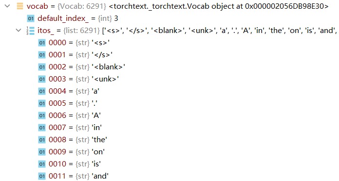
The special tokens <s>, </s>, <blank>, and <unk> are vocabulary entries
with their own IDs.
0x04 Converting text to tensors
After vocabulary lookup, dataset strings become ID tensors:
processed_src = torch.cat(
    [
        bs_id,
        torch.tensor(src_vocab(src_pipeline(_src)), dtype=torch.int64),
        eos_id,
    ],
    dim=0,
)

processed_tgt = torch.cat(
    [
        bs_id,
        torch.tensor(tgt_vocab(tgt_pipeline(_tgt)), dtype=torch.int64),
        eos_id,
    ],
    dim=0,
)
Then the data path pads and stacks examples:
single source example:
    [BOS, ..., EOS] -> [L]

padded source batch:
    src -> [B,S]

padded target batch:
    tgt -> [B,T]
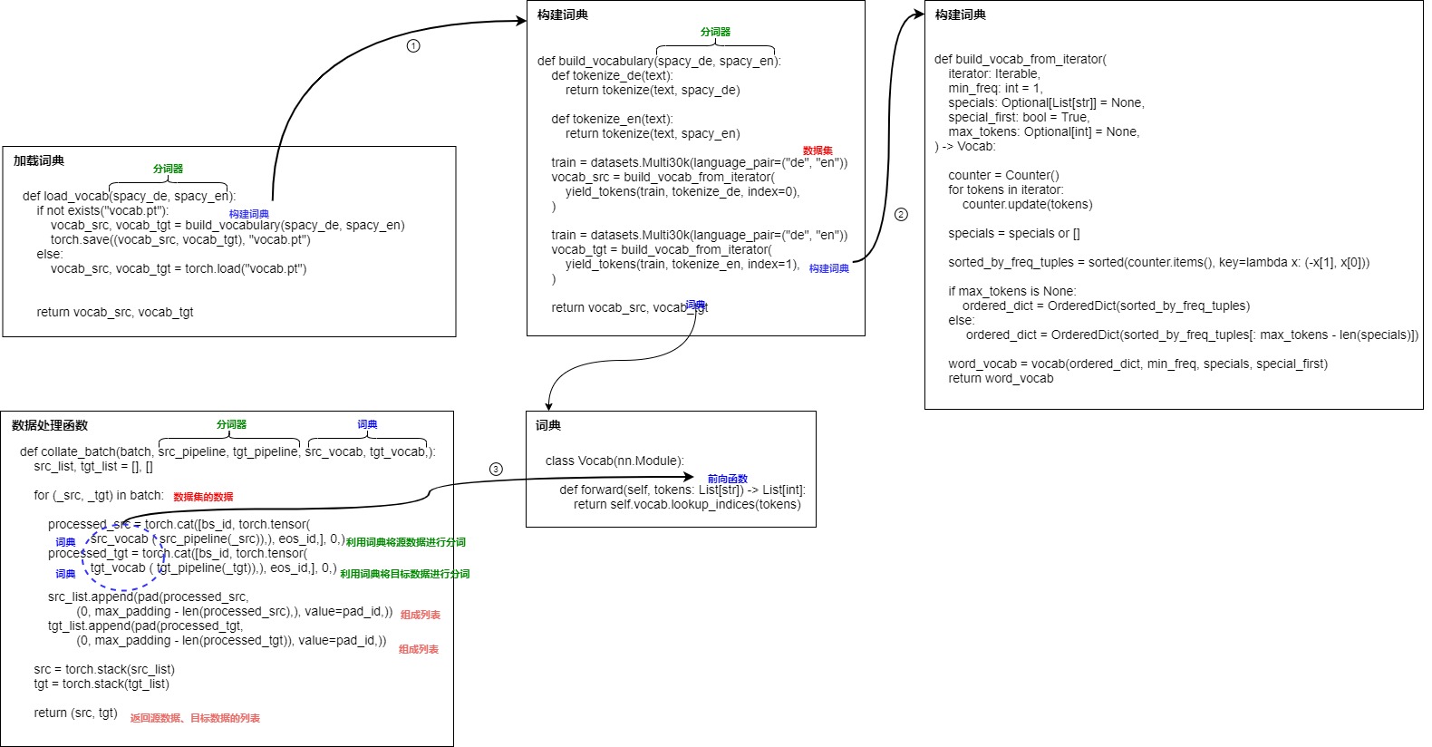
The data path is:
raw dataset string
    -> token strings
        -> vocabulary IDs
            -> padded ID tensors
The training loop uses these tensors to construct shifted inputs, labels, causal masks, and loss counts. We will examine the alignment needed for that step when building padded and packed batches.
0x04A Keeping metadata with the IDs
Returning only list[int] discards information that later stages otherwise
have to guess. A useful pre-batch contract is:
@dataclass
class EncodedSequence:
    input_ids: list[int]
    special_tokens_mask: list[bool]
    offsets: list[TokenOffset | None]
    sequence_ids: list[int | None]
    tokenizer_hash: str
    template_hash: str | None
    original_length: int
    truncated: bool

    def validate(self, vocab_size: int) -> None:
        n = len(self.input_ids)
        assert len(self.special_tokens_mask) == n
        assert len(self.offsets) == n
        assert len(self.sequence_ids) == n
        assert all(0 <= token_id < vocab_size for token_id in self.input_ids)
        assert all(
            offset is None or offset.start <= offset.end
            for offset in self.offsets
        )
Special tokens commonly have offset=None because they were not copied from a
source span. In pair encoders, sequence_ids may use 0 for the first source,
1 for the second, and None for inserted control tokens. A single attention
mask cannot recover these distinctions.
After collation, the tensor contract becomes:
input_ids               [B,S] int64 or implementation-supported integer type
attention_mask          [B,S] bool/int, 1 for model-visible content/control rows
special_tokens_mask     [B,S] bool
sequence_ids            [B,S] int with sentinel for inserted/padded rows
position_ids            [B,S] integer, constructed later under M3.3's policy
lengths                 [B]   number of non-padding rows
attention_mask=1 does not mean “ordinary content token.” BOS, EOS, separators,
and role markers can be visible to the model while also being marked special.
0x04B Padding and batching
A DataLoader collects examples and passes them to collate_fn. The collator
converts the list into tensors for the training loop:
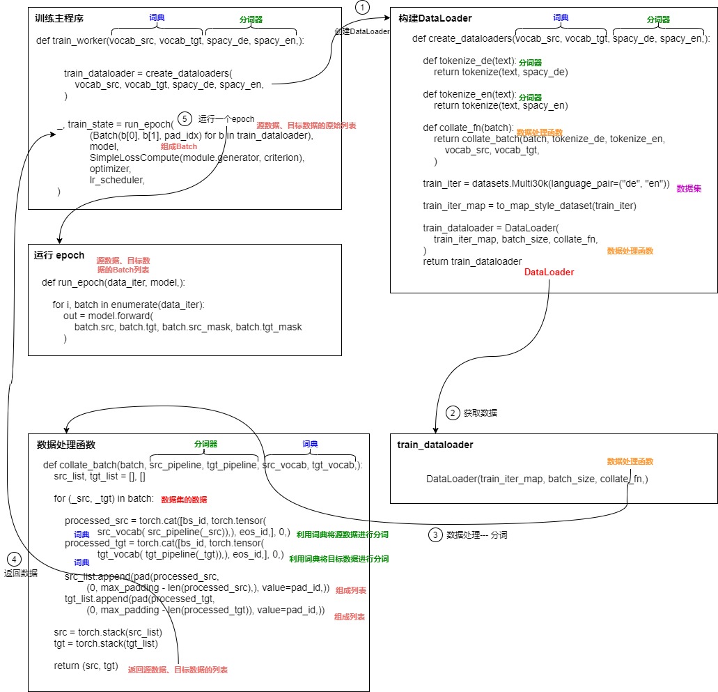
For a batch of encoded lengths l_1,...,l_B, ordinary padding chooses:
then writes every example into a [B,S_batch] rectangle. The fraction of token
slots that contain real sequence rows is:
This is a batching efficiency measure, not model accuracy. Length bucketing can
raise eta_tokens by grouping examples with similar lengths. Fixed global
padding usually wastes more slots.
def collate_encoded(examples, pad_id, max_length, padding_side="right"):
    lengths = [min(len(x.input_ids), max_length) for x in examples]
    S = max(lengths)

    ids = torch.full((len(examples), S), pad_id, dtype=torch.long)
    visible = torch.zeros((len(examples), S), dtype=torch.bool)
    special = torch.ones((len(examples), S), dtype=torch.bool)

    for row, (example, length) in enumerate(zip(examples, lengths)):
        content = torch.tensor(example.input_ids[:length])
        content_special = torch.tensor(example.special_tokens_mask[:length])

        start = 0 if padding_side == "right" else S - length
        stop = start + length
        ids[row, start:stop] = content
        visible[row, start:stop] = True
        special[row, start:stop] = content_special

    return {
        "input_ids": ids,
        "attention_mask": visible,
        "special_tokens_mask": special,
        "lengths": torch.tensor(lengths),
    }
The implementation must define whether truncation happens before or after template insertion. Those policies produce different sequences:
truncate content, then add EOS:
    required EOS is preserved

add EOS, then truncate right edge:
    EOS may disappear
Neither is universally correct; the training format decides. The choice must be explicit and tested.
Left padding, right padding, and packing
A generation loop that reads the last column’s logits needs the last real token in that column. Left padding provides that arrangement:
right padding:
    common in encoder training and many packed/unpacked training paths

left padding:
    convenient for batched generation when the last physical column must be
    the last valid prefix token

padding-free packing:
    concatenates examples while carrying segment boundaries / cumulative
    lengths so attention cannot cross examples
A runtime can also gather each row’s last valid position, allowing right padding. With left padding, position IDs must account for the leading PAD columns. Either approach needs correct lengths and padding-side metadata.
Packing removes pad rows but adds a stronger boundary contract. For sequences
with lengths [3,2,4]:
packed IDs:
    [a0 a1 a2 | b0 b1 | c0 c1 c2 c3]

cu_seqlens:
    [0, 3, 5, 9]
An optimized attention kernel can consume cu_seqlens; a dense reference path
can construct a block-diagonal mask. Omitting boundaries silently lets one
document attend into another.
Reproducing distributed loading
DistributedSampler partitions examples across ranks. It does not define
tokenization, padding, or deterministic shuffling by itself. A reproducible
epoch records:
dataset/shard manifest
sampler seed and epoch
rank/world size
tokenizer and template hashes
length-bucketing policy
drop_last policy
The collator should be pure with respect to an encoded example: changing rank must not change its token IDs. Stochastic subword regularization is an exception only when its per-example RNG stream is intentionally keyed and recorded.
0x05 Words, characters, subwords, and bytes
Tokenization is a compression and coverage tradeoff. The same raw text can be cut at different granularities:
A word vocabulary represents familiar words compactly. Covering every new word, name, or inflection, however, would require continual growth or an unknown-token fallback.
Characters can combine into unfamiliar words using fewer vocabulary entries, but each word occupies more sequence positions. Character handling still needs rules for Unicode normalization and grapheme boundaries. Bytes provide a base alphabet of just 256 values that covers UTF-8 text, though a single character may occupy several byte positions.
Subwords combine frequent fragments to shorten those sequences while retaining smaller pieces for rare forms. Their boundaries need not match linguistic words or morphemes, and compression can vary substantially across languages and domains.
For example:
"unbelievable"
might become:
word-level:
    ["unbelievable"]

character-level:
    ["u", "n", "b", "e", "l", "i", "e", "v", "a", "b", "l", "e"]

subword-level:
    ["un", "believ", "able"]

byte-level:
    UTF-8 bytes, then possible byte-level merges
Subword tokenizers became the practical compromise because they can represent rare words without assigning every possible word a dedicated vocabulary entry, while still compressing common fragments.
0x06 BPE training: learn the merge table
BPE begins as a compression procedure:
find a frequent adjacent pair
replace it with a new symbol
repeat
The name covers related algorithms, not one universal trainer. Gage’s 1994 compression procedure replaces frequent byte pairs with unused byte values. Sennrich et al. adapt that operation to word segmentation: words begin as character sequences with an end-of-word marker, pair statistics are weighted by word frequency, and merges do not cross word boundaries. Modern causal-LM tokenizers often begin from bytes but impose regex or pre-token boundaries before counting and applying merges. The shared operation is pair replacement; the counted units, boundaries, base alphabet, stopping rule, and serialized IDs are separate design choices (Gage, 1994, Sennrich et al., 2016).
At each training step, BPE counts adjacent pairs and merges the selected pair. The resulting ordered merge table is saved for encoding new text.
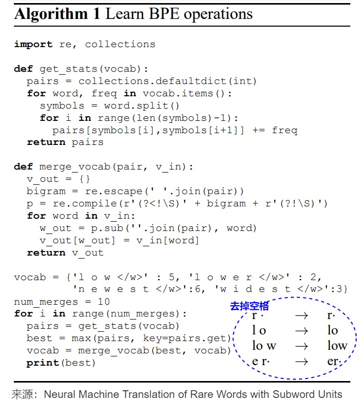
A byte-level BasicTokenizer version makes the training object precise:
class BasicTokenizer(Tokenizer):
    def train(self, text, vocab_size, verbose=False):
        assert vocab_size >= 256
        num_merges = vocab_size - 256

        text_bytes = text.encode("utf-8")
        ids = list(text_bytes)

        merges = {}
        vocab = {idx: bytes([idx]) for idx in range(256)}

        for i in range(num_merges):
            stats = get_stats(ids)
            pair = max(stats, key=stats.get)
            idx = 256 + i

            ids = merge(ids, pair, idx)
            merges[pair] = idx
            vocab[idx] = vocab[pair[0]] + vocab[pair[1]]

        self.merges = merges
        self.vocab = vocab
The line max(stats, key=stats.get) leaves tie-breaking dependent on insertion
order. When two pairs have equal counts, Python returns the first maximum in the
dictionary’s iteration order. That order is stable only if pair insertion,
corpus iteration, chunk iteration, and runtime behavior are all fixed. A
different parallel reduction can produce another first merge and therefore a
different rank table.
The same line fails when no adjacent pairs remain. For the text aaaa, the
first merge turns the four bytes into two aa IDs and the second joins them
into one ID. A third merge finds an empty dictionary, and max raises
ValueError. A trainer must either stop when no pair remains, returning a
smaller vocabulary than requested, or reject the requested size.
The initial vocabulary has 256 byte values. Each merge creates a new ID:
new_id = 256 + merge_index
and records:
merges[(old_id_a, old_id_b)] = new_id
vocab[new_id] = vocab[old_id_a] + vocab[old_id_b]
For a small word-level teaching example, suppose the corpus counts are:
low      x 5
lower    x 2
newest   x 6
widest   x 3
One initial segmentation is:
low     -> l o w </w>
lower   -> l o w e r </w>
newest  -> n e w e s t </w>
widest  -> w i d e s t </w>
Pair counts are weighted by word frequency. If (e, s) and (s, t) tie, the
implementation’s tie-break determines which is merged first and must be fixed
to reproduce the result.
The training equation is:
pair* = argmax_pair count(pair)
ids = rewrite(ids, pair*, new_id)
This procedure learns a vocabulary from corpus counts. The Transformer’s weights are trained separately, using the resulting ID sequences.
Deriving weighted BPE pair counts
The frequency of a pair is counted over corpus occurrences, not merely over
distinct vocabulary entries. Let W be the set of pre-tokenized word forms,
f(w) their corpus frequencies, and count_w(a,b) the number of adjacent
occurrences of pair (a,b) in the current segmentation of w. Then:
The next merge is:
Why the frequency multiplier? If low occurs five times, the pair (l,o)
contributes five opportunities for compression. Treating every distinct word
once would optimize the type list, not the token stream on which the tokenizer
will operate.
For the teaching corpus:
low      x 5 -> l o w </w>
lower    x 2 -> l o w e r </w>
newest   x 6 -> n e w e s t </w>
widest   x 3 -> w i d e s t </w>
the initial contribution to (l,o) is 5 + 2 = 7, because both low and
lower contain that pair. After a merge, pair counts must be updated around
every replaced occurrence because new adjacencies appear.
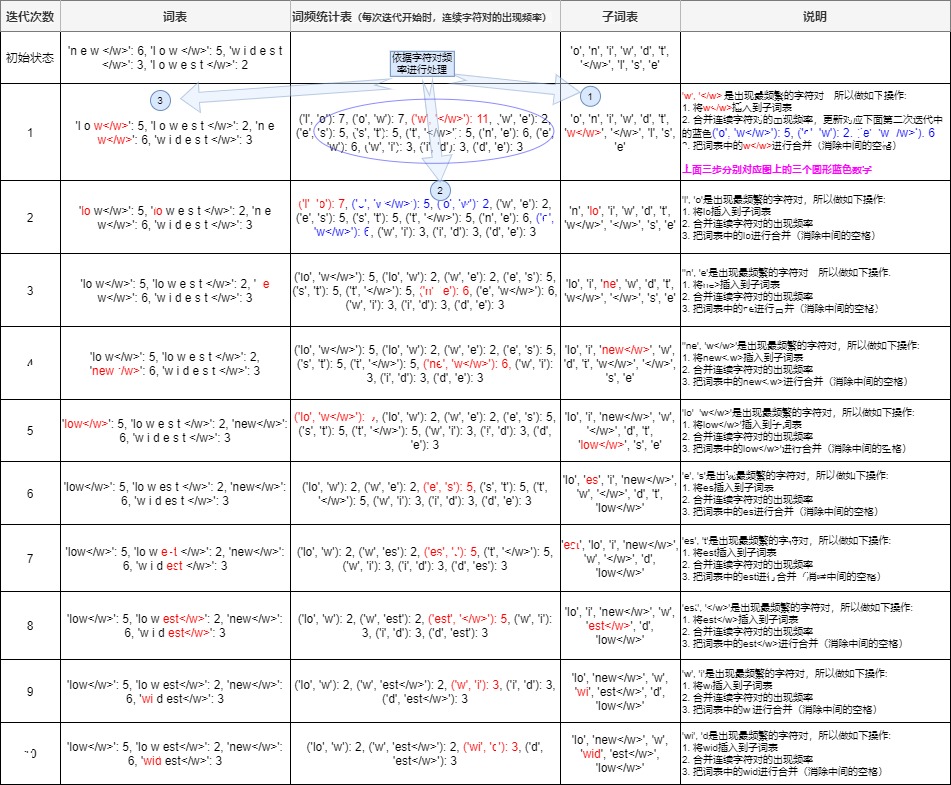
The figure illustrates the merge steps. A reproducible implementation also fixes normalization, boundaries, byte fallback, tie-breaking, and serialization.
Updating the training sequence
Let the pre-tokenized training state at merge round be:
where is the corpus frequency of independent unit and is its current symbol sequence. Pair score is computed inside each unit:
There is no term joining the final symbol of unit to the first symbol of unit . If units are words, regex spans, or user-declared chunks, flattening them silently trains a different tokenizer.
The score still does not identify one pair when several maxima tie. This reference implementation breaks ties by comparing the pairs of numeric IDs lexicographically:
That rule is not claimed to be universal. The released subword-nmt
implementation uses (frequency, pair) as the key to max, selecting the
lexicographically largest pair among equal counts; MinBPE’s teaching trainer
uses first encounter. Either can be deterministic when fully declared, but
they are not artifact-equivalent
(learn_bpe.py,
minbpe/basic.py).
Counting and replacing overlapping pairs
Pair counting uses adjacent windows, so windows may overlap. Rewriting one round must instead choose non-overlapping occurrences. For a run of copies of symbol :
For a a a, (a,a) therefore has two windows but a left-to-right rewrite can
replace only the first two symbols:
count:      [a a] a    and    a [a a]    -> score 2
rewrite:    [a a] a -> X a                  -> 1 replacement
not:        X X
The score selects the rule; the number of legal replacements determines the actual reduction in training-stream length. If is the weighted number of non-overlapping replacements in round , then:
Counting overlapping windows as simultaneous replacements overstates the reduction in sequence length and can make an optimized trainer disagree with the reference.
Following three merge rounds
The constructed example uses four base byte addresses:
0 = a    1 = b    2 = c    3 = d

independent training units:
    [a a a b]       frequency 2
    [d a a a b a c] frequency 1

contract:
    count weighted overlapping windows inside each unit
    rewrite left-to-right without overlap
    break equal scores by ascending (left_id, right_id)
    new_id = V_base + rank
    stop when score < 2 or after 4 merges
The first score for (a,a) is six: two overlapping windows in each occurrence
of aaab, weighted by two, plus two windows in daaabac. Only three weighted
replacements are legal. The complete trace is:
At rank 0, the pair (0,0) has score six. Three legal replacements create
4=X=aa, changing aaab x2; daaabac x1 to Xab x2; dXabac x1 and reducing
the weighted length from 15 to 12.
At rank 1, C(a,b)=C(X,a)=3. The numeric tie-break selects (0,1), creating
5=Y=ab. The units become XY x2; dXYac x1, and the length falls to 9.
At rank 2, (4,5) has score three and three replacements create
6=Z=aaab. The units become Z x2; dZac x1, with weighted length 6.
The best remaining score is one, so min_frequency=2 stops training without
creating another row.
This small constructed example tests the merge rules; it does not measure production performance.
Updating only the affected counts
A simple trainer recounts every unit after every merge:
for rank in range(max_merges):
    counts = weighted_pair_counts(units)
    pair, score = min(
        counts.items(),
        key=lambda item: (-item[1], item[0][0], item[0][1]),
    )
    if score < min_frequency:
        break

    new_id = base_size + rank
    units = [
        rewrite_left_to_right(unit, pair, new_id)
        for unit in units
    ]
    merge_records.append((rank, pair, new_id))
A scalable trainer can instead cache one pair counter per unit, maintain a
global weighted counter and pair -> affected units index, and recount only
units containing the selected pair:
affected = sorted(pair_to_units[selected_pair])
for unit_id in affected:
    for pair, count in local_counts[unit_id].items():
        global_counts[pair] -= frequency[unit_id] * count

    units[unit_id] = rewrite_left_to_right(
        units[unit_id], selected_pair, new_id
    )
    local_counts[unit_id] = count_pairs(units[unit_id])

    for pair, count in local_counts[unit_id].items():
        global_counts[pair] += frequency[unit_id] * count

    refresh_pair_to_units(unit_id)
Both implementations must produce the same ordered merges, IDs, pieces, stopping reason, final training sequences, and golden encodings. Comparing their outputs checks that the optimization preserves the algorithm.
When training stops
vocab_size is not always “256 plus exactly this many successful merges.” A
trainer may reserve special rows, include an initial alphabet, stop because no
pair reaches min_frequency, or reject pieces beyond a maximum length. Hugging
Face’s BpeTrainer, for example, defines vocab_size as the final size
including alphabet and special tokens and separately exposes
min_frequency, limit_alphabet, initial_alphabet, boundary prefix/suffix,
and max_token_length
(official trainer API).
If base, merge-created, and reserved address sets are disjoint, the vocabulary size is:
The inequality matters. In the synthetic trace, four merges were permitted but only three were learned because the next score fell below two. Also distinguish the persistent address vocabulary from symbols still visible in the rewritten training stream: a base symbol can disappear from the final segmentation while its address remains necessary to decode merge ancestry or cover future input.
Where merges are allowed
In Sennrich-style BPE, each word begins as characters plus a word-final marker. Merges stay inside the word, preserving the original word boundaries. A flat byte implementation instead treats an entire input string as one unit; without extra boundaries, it can merge across spaces, punctuation, or document joins.
A regex-bounded implementation first splits the text into spans and permits byte merges only within each span. Training and encoding must use the same pattern. For joint multilingual BPE, languages share the base alphabet and merge table, so their corpus weights affect the pair counts and the resulting priorities.
OpenAI’s released GPT-2 encoder applies a regex split, converts each span to a
reversible byte-to-Unicode representation, and then applies the lowest-rank
available merge inside that span. MinBPE’s BasicTokenizer intentionally omits
that split, while RegexTokenizer restores it. These are useful reference
implementations, not evidence that every modern tokenizer uses the same pattern
(GPT-2 encoder.py,
MinBPE).
BPE-dropout keeps the learned merge table but randomly skips eligible merges while preparing model-training sequences. At zero dropout it reduces to ordinary BPE; otherwise reproducibility also depends on the RNG policy and seed (Provilkov et al., 2020).
A minimal pair-count and rewrite implementation
def get_stats(ids, counts=None):
    counts = {} if counts is None else counts
    for left, right in zip(ids, ids[1:]):
        pair = (left, right)
        counts[pair] = counts.get(pair, 0) + 1
    return counts


def merge(ids, pair, new_id):
    out = []
    i = 0
    while i < len(ids):
        if i + 1 < len(ids) and (ids[i], ids[i + 1]) == pair:
            out.append(new_id)
            i += 2
        else:
            out.append(ids[i])
            i += 1
    return out
This simple implementation rescans the sequence at every round. With M
rounds and N_m symbols remaining at round m, its work is roughly:
which is O(MN) under the loose bound N_m <= N. Production trainers avoid a
full recount for every round by maintaining occurrence lists, pair counts, and
priority structures, then invalidating or updating only neighborhoods touched
by a merge. That optimization changes bookkeeping, not the learned contract:
the chosen pair and deterministic tie-break must remain equivalent.
Saving merge order
Consider two learned rules:
(a,b) -> X at rank 3
(b,c) -> Y at rank 9
For a b c, both pairs are present, but rank 3 must be applied first. Storing
only the unordered set {(a,b),(b,c)} cannot reproduce encoding. The serialized
model must preserve rank or equivalent priority.
MinBPE makes a useful artifact distinction:
.model:
    pattern, special tokens, and ordered merge rules required to encode/decode

.vocab:
    human-readable rendering useful for inspection, not sufficient as model state
A robust loader validates:
assert sorted(merges.values()) == list(range(256, 256 + len(merges)))
assert len(vocab) == 256 + len(merges)
assert all(new_id not in special_ids for new_id in merges.values())
If two training implementations resolve equal counts differently, they produce different rank tables even if both end at the same vocabulary size. A reproduction test therefore compares encoded IDs on a golden corpus, not just the number of rows.
0x07 BPE use: apply learned merge ranks
Encoding uses the merge priorities learned during training. It finds which saved rules apply to the current sequence and selects by rank; it does not recount pair frequencies in the new input.
Longest-match selection, as used by WordPiece, follows a different rule. In BPE, a longer piece may become available only after its parent pieces have been merged.
Selecting the next merge
Let one admitted pre-token become a base-symbol sequence
For byte-level BPE, each initial symbol is a byte ID in
{0,...,255}. For character BPE it may instead be a character-alphabet ID.
The distinction was fixed by the artifact before this loop begins.
Each learned record has the form
where is the merge rank, are parent IDs, is the new ID, and is its byte sequence. Checking these bytes lets a loader verify that merge ancestry agrees with the decoder vocabulary.
At state , the eligible locations are
The reference implementation selects
rewrites that occurrence, and recomputes eligibility:
The second coordinate makes leftmost occurrence the explicit tie-break for this implementation. The first coordinate explains why current-input frequency is absent: frequency learned the ranks during fitting; rank controls application.
The merge loop can be summarized as:
eligible = adjacent pairs present in the frozen merge table
choice   = minimum (learned_rank, left_position)
rewrite  = one occurrence, then recompute
stop     = no eligible adjacent pair remains
Encoding abc and abab
Use a byte alphabet with these synthetic records:
- Rank
0mergesa(97)andb(98)into ID256, whose bytes are61 62(ab). - Rank
1mergesb(98)andc(99)into ID257, with bytes62 63(bc). - Rank
2mergesab(256)andc(99)into ID258, with bytes61 62 63(abc). - Rank
3merges twoab(256)pieces into ID259, with bytes61 62 61 62(abab).
For abc, two pairs are initially visible:
state [97, 98, 99]
      [ a,  b,  c]

candidate at 0: (97, 98) -> 256, rank 0
candidate at 1: (98, 99) -> 257, rank 1
Rank 0 wins:
[97, 98, 99] -> [256, 99] -> [258]
     ab               abc
Choosing the longest currently known vocabulary entry cannot justify the first
step, because abc is not yet an adjacent pair. Choosing rank 1 first would
produce [97,257], or a + bc, and make rank 2 unreachable. All three
outputs decode to the same bytes, but only one has the checkpoint’s token IDs.
The repeated input abab adds an overlap and ancestry check:
[a,b,a,b]
    -> [ab,a,b]
    -> [ab,ab]
    -> [abab]

[97,98,97,98] -> [256,97,98] -> [256,256] -> [259]
Each merge can expose another eligible pair, so the saved priority order determines which pieces are formed next.
Comparing merge schedules
Real implementations expose several related schedules:
The educational tiktoken implementation merges one minimum-rank occurrence,
then updates the candidates. GPT-2’s public encoder chooses a pair type and
replaces all its non-overlapping occurrences before selecting again. A fixed
rule schedule instead visits each learned rule in rank order and applies it
exhaustively once.
An optimized occurrence-based implementation can maintain candidates in a priority queue. It performs the same local merges as the first approach, while discarding queue entries made stale by earlier changes.
For a proper merge table learned from existing parents in ascending order,
these forms commonly agree. All four give the same IDs for abc, abab,
split UTF-8 bytes, declared boundaries, and unmerged bytes. This agreement
holds for these cases; it is not a theorem about every file called a BPE
vocabulary.
An intentionally improper dictionary separates the contracts:
rank 0: (256, a) -> 257
rank 1: (a, a)   -> 256
input:  a a a a

dynamic occurrence priority:
    [257, 97]

selected-pair rounds or one fixed rule schedule:
    [256, 256]
Rank 0 depends on a symbol created only by the later rank. A dynamic scheduler can revisit it; a one-pass schedule cannot. The formal BPE analysis is useful precisely because production families differ in their formal application semantics. Loaders should therefore name the implementation family and validate golden IDs instead of assuming that any rank map can be consumed by any BPE loop.
Implementing the merge loop
This implementation rescans the current IDs:
def encode_reference(unit_bytes, merge_rank):
    ids = list(unit_bytes)

    while len(ids) > 1:
        candidates = []
        for left_pos, (left_id, right_id) in enumerate(zip(ids, ids[1:])):
            record = merge_rank.get((left_id, right_id))
            if record is not None:
                candidates.append(
                    (record.rank, left_pos, record.new_id)
                )

        if not candidates:
            break

        _, left_pos, new_id = min(candidates)
        ids[left_pos:left_pos + 2] = [new_id]

    return ids
For a pre-token of base symbols and successful merges, repeated full scans perform
which reaches when . This is a pedagogical implementation, not a production complexity promise.
An optimized occurrence-priority implementation keeps:
values: int32[N]             current token ID stored at each original node
prev, next: int32[N]         linked-list adjacency
alive: bool[N]               whether a node remains in the sequence
heap entry:
    (rank, left_position, right_position,
     expected_left_id, expected_right_id, new_id)
The heap trace for abc is:
initial nodes:
    index     0      1      2
    values   97     98     99
    next      1      2     -1

heap:
    (rank 0, left 0, right 1, 97, 98, 256)
    (rank 1, left 1, right 2, 98, 99, 257)

pop rank 0:
    values[0] = 256
    alive[1] = false
    next[0] = 2; prev[2] = 0
    push new local pair (256, 99), rank 2

old rank-1 entry:
    stale because node 1 is dead -> discard

pop rank 2:
    values[0] = 258
    alive[2] = false
    output traversal -> [258]
Every popped entry must revalidate liveness, adjacency, and expected IDs. A heap without stale-entry validation can merge nodes that are no longer neighbors. With bounded local updates, this implementation performs candidate insertions and heap work. That bound belongs to this data structure and contract; production tokenizers may use different layouts, batching, SIMD, or specialized algorithms.
Reconstructing bytes and text
Byte-level BPE contains two distinct transformations:
text codec:
    Unicode text -> UTF-8 bytes

piece codec:
    bytes <-> token IDs under the ranked merge artifact
GPT-2’s public implementation first maps all 256 bytes to a reversible Unicode
alphabet so its regex and string machinery can carry byte values, then runs BPE
and reverses that map during decode. Modern tiktoken exposes mergeable byte
sequences directly. The byte-to-Unicode layer is therefore an implementation
indirection used by GPT-2, not a mathematical requirement of BPE.
Byte decoding concatenates the byte pieces in ID order:
where is the byte piece assigned to ID . Text rendering happens only after the complete byte stream exists:
RFC 3629 encodes one Unicode scalar as one to four bytes. A token boundary need not coincide with that scalar boundary. For the euro sign:
UTF-8 text:        €
bytes:             E2 82 AC
token 260 bytes:  E2 82       # incomplete by itself
token 172 bytes:  AC

decode_bytes([260])      -> E2 82
strict UTF-8             -> error
replacement UTF-8       -> U+FFFD

decode_bytes([260,172])  -> E2 82 AC
strict UTF-8             -> €
Inspecting token bytes reveals incomplete characters. Decoding each token to
text separately can insert replacement characters before the remaining bytes
arrive, so concatenating those strings may not recover the input.
errors="replace" is a lossy display or recovery policy.
Encoding a stream of bytes
Transport chunks are not tokenizer boundaries. In general,
because a regex pre-token, UTF-8 scalar, special-token delimiter, or learned merge may cross the transport split.
The synthetic a | b | c stream makes the instability visible:
After receiving a, the provisional result is [97]. Receiving b changes
it to [256]; receiving c changes it again to [258]. This encoder emits
nothing until the declared boundary after abc, when [258] becomes safe to
return.
Encoding the three chunks independently would emit [97,98,99]. Those IDs
decode to the same bytes but are not the canonical encoding [258]. A split
euro sign exhibits both hazards: E2 | 82 | AC crosses a UTF-8 boundary and
the learned (E2,82) merge.
A conservative stream encoder therefore carries explicit state:
StreamState:
    committed_ids       IDs whose complete unit boundary is final
    undecided_bytes     bytes that later input may retokenize
    pretoken_state      regex/rule state and open pre-token
    utf8_state          pending continuation-byte requirement
    special_state       partial reserved-token delimiter, if applicable
Its safest baseline is:
def push_chunk(state, chunk, unit_boundary=False):
    state.undecided_bytes += chunk
    state.provisional_ids = encode_unit(state.undecided_bytes)

    if not unit_boundary:
        return []

    emitted = state.provisional_ids
    state.committed_ids.extend(emitted)
    state.undecided_bytes = b""
    state.provisional_ids = []
    return emitted
That policy may buffer more than necessary, but its correctness argument is simple. More aggressive choices require stronger proof:
Buffering a whole pre-token matches batch encoding when the boundary detector is reliable. Retokenizing only a suffix can reduce latency and memory use, but requires a tokenizer-specific bound beyond which earlier IDs cannot change.
An API such as encode_with_unstable can expose a stable prefix and possible
completions; callers must follow its particular, explicitly unstable API.
Dedicated incremental BPE algorithms offer another approach, provided their
merge semantics, dictionary assumptions, and implementation match the deployed
tokenizer.
The 2026 Incremental BPE Tokenization paper reports an exact incremental algorithm with polylogarithmic per-byte work under its formal contract. This is a recent, source-reported result, not permission to apply a fixed suffix heuristic to GPT-2, SentencePiece, or every ranked merge file. BLT makes the same architectural pressure visible from another direction: BPE boundaries are not naturally final as bytes arrive (BLT).
A streaming encoder must hold back any ID that later bytes could change.
Section 0x0D follows these stable IDs into request processing, caching, and
output handling.
0x08 WordPiece, Unigram, and SentencePiece
WordPiece selects the longest legal match at each position. Unigram scores complete segmentations and can choose or sample a path. SentencePiece packages a Unigram, BPE, character, or word model with normalization, vocabulary storage, and decoding. Sampling a segmentation while preparing training data, as BPE-Dropout and Unigram sampling do, adds a random state that must be replayable.
All of these return the same kind of output, a sequence of integer IDs, while running different programs. The subsections that follow answer five questions for each method:
What evidence defines vocabulary fitting?
What state is serialized?
What recurrence runs during encoding?
What happens when coverage fails?
What randomness, if any, is part of training and evaluation?
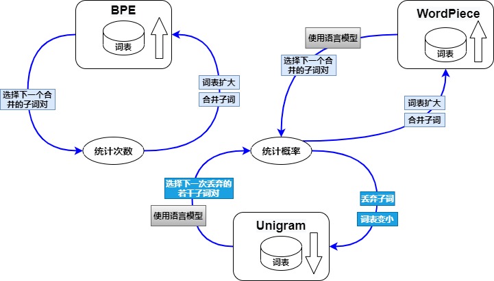
The following diagram compares how three of the methods build their vocabularies. In it, BPE counts pairs and merges the most frequent one, WordPiece also merges pairs but uses a language model to choose them, and Unigram uses a language model to choose pieces to discard, so its vocabulary shrinks. The diagram is an orientation, not a complete specification of any method.
Learning a WordPiece vocabulary
WordPiece was used in speech-recognition work such as Japanese and Korean Voice Search. Common teaching reconstructions grow a vocabulary from small pieces, scoring additions by a likelihood gain or a cohesion-like ratio. The released encoder alone does not determine which training recipe produced its vocabulary.
The official BERT repository
releases vocab.txt and the Python encoder, but not the original C++ vocabulary
trainer. Public teaching implementations often score a candidate pair (a,b)
with a ratio such as:
which discounts pairs that are frequent only because their individual pieces are common. Other implementations optimize related likelihood criteria or use different initialization, continuation marking, tie-breaks, and stopping rules. To reproduce encoding, use the released vocabulary, normalizer, pre-tokenizer, continuation syntax, fallback rule, and ID order. Reconstructing the unpublished trainer is a separate task.
Encoding with WordPiece
After upstream normalization and pre-tokenization, let x be one pre-token of
length n. BERT-style WordPiece has one lookup domain for word-initial pieces
and another for continuation pieces prefixed by ##. At position i, choose:
where:
The max is why the algorithm is longest-match-first. It is not maximizing the
sum of scores over a complete lattice, and it is not applying ranked merge
rules. If the set is empty at any position, the BERT-style policy returns one
[UNK] for the whole pre-token, not the successfully matched prefix plus an
unknown suffix.
For this example, use the following vocabulary:
initial root:       un, runn, play, ,
continuation root:  ##want, ##ed, ##ing, ##er
fallback:           [UNK]
We can now follow unwanted through the search.
At position 0, searching from unwanted down to shorter prefixes finds
un, so the output starts with [1]. At position 2, continuation search
starts with ##wanted and finds ##want, extending the output to [1,2].
At position 6, ##ed consumes the remainder and gives [1,2,3].
In contrast, want cannot use ##want at position zero, and playingx
matches play before reaching an uncovered suffix. Both become [UNK] under
the declared whole-pre-token fallback. Unwanted also becomes [UNK] in the
cased path but succeeds after the separately declared lowercase normalizer.
def wordpiece_reference(word, initial_vocab, continuation_vocab, unk):
    output = []
    start = 0

    while start < len(word):
        vocab = initial_vocab if start == 0 else continuation_vocab
        terminal = None

        for end in range(len(word), start, -1):
            surface = word[start:end]
            if surface in vocab:
                terminal = (end, vocab[surface])
                break

        if terminal is None:
            return [unk]  # discard every partial match for this pre-token

        start, token_id = terminal
        output.append(token_id)

    return output
The simple reference loop repeatedly slices substrings. A more realistic
matcher stores characters as chars[n] and the vocabulary as trie arrays such
as:
next[node, character] -> child_node or missing
terminal_id[node]     -> vocabulary ID or missing
root_initial          -> pieces legal at position 0
root_continuation     -> pieces legal after position 0
At each cursor, walk the appropriate trie and retain the deepest terminal. This gives the same IDs as substring search. Check both implementations on continuations, punctuation, normalization, uncovered suffixes, and inputs over the configured length limit.
Accelerating WordPiece search
A plain restart-from-root trie can still repeat work after failed long matches. The Fast WordPiece paper describes an Aho-Corasick-inspired trie with failure transitions and output links. Its key result is a strict linear-time algorithm in input length under the paper’s contract, including a general-text variant that combines pre-tokenization and WordPiece matching.
Fast WordPiece preserves longest-match behavior while changing the search structure. It does not define vocabulary training, and its reported timings depend on the implementation and workload.
Learning Unigram piece probabilities
Unigram reverses BPE’s vocabulary direction. It begins with an overcomplete candidate set, estimates piece probabilities, and repeatedly prunes candidates until a target size is reached. The difficult part is the training objective. The segmentation is latent, so training cannot silently replace all possible segmentations with one greedy path.
Let S(x) be every piece sequence that concatenates exactly to string x. For
one segmentation z=(z_1,...,z_m), the model assumes independent piece draws:
The segmentation is not observed in the raw corpus. Marginalizing it gives:
and corpus training minimizes:
where c(x) is the corpus multiplicity. The sum includes every segmentation
that can produce the string. Replacing it by the largest term, as in Viterbi,
would fit a different model.
Forward and backward probabilities
Enumerating all segmentations is exponential in the worst case, but their
shared prefixes and suffixes form a directed acyclic graph over string
positions. Define an edge (i,z,j) when piece z exactly covers x[i:j].
The forward recurrence is:
The backward recurrence is:
Both meet at the same marginal:
The three factors in alpha[i] * p(z) * beta[j] enumerate every complete path
that uses edge (i,z,j): a prefix reaching i, the edge itself, and a suffix
from j. Dividing by the total therefore yields the posterior probability that
the latent segmentation used that edge:
Summing these edge posteriors produces the expected count for piece z:
For the simplest maximum-likelihood M-step, maximize
sum_z c_hat(z) log p(z) under sum_z p(z)=1. Differentiating the Lagrangian
with respect to p(z) gives c_hat(z)/p(z)=lambda; summing over z gives
lambda=sum_u c_hat(u), hence:
That derivation is the baseline contract. SentencePiece’s production trainer contains additional priors, digamma-based updates, thresholds, sub-iterations, and numerical safeguards. The baseline must not be presented as a line-for-line description of its C++ M-step.
def forward_backward(text, pieces):
    alpha = [0.0] * (len(text) + 1)
    beta = [0.0] * (len(text) + 1)
    alpha[0] = 1.0

    edges = build_lattice_edges(text, pieces)
    for end in range(1, len(text) + 1):
        for start, piece in incoming(edges, end):
            alpha[end] += alpha[start] * piece.probability

    beta[-1] = 1.0
    for start in reversed(range(len(text))):
        for piece, end in outgoing(edges, start):
            beta[start] += piece.probability * beta[end]

    total = alpha[-1]
    expected = {piece.id: 0.0 for piece in pieces}
    for start, piece, end in edges:
        posterior = alpha[start] * piece.probability * beta[end] / total
        expected[piece.id] += posterior

    return total, expected
The production implementation should use log-space or scaled arithmetic for long strings. The reference calculation uses exact rational numbers to avoid underflow and distinguish mathematical errors from floating-point rounding.
Segmenting abab
For a small worked example, use the following vocabulary.
Assign a and b IDs 0 and 1, each with probability 1/4; these two
pieces are required for character coverage. The optional pieces are ab
(ID 2, probability 7/20), aba (ID 3, probability 1/10), and bab
(ID 4, probability 1/20).
The six complete paths are:
P(a b a b) = (1/4)^4             = 1/256
P(a b ab)  = (1/4)(1/4)(7/20)     = 7/320
P(a bab)   = (1/4)(1/20)          = 1/80
P(ab a b)  = (7/20)(1/4)(1/4)     = 7/320
P(ab ab)   = (7/20)^2             = 49/400
P(aba b)   = (1/10)(1/4)          = 1/40
Their sum is:
The independently computed forward and backward arrays are:
alpha = [1, 1/4, 33/80, 13/64, 1329/6400]
beta  = [1329/6400, 49/320, 33/80, 1/4, 1]
For example, the posterior for the first ab edge from position 0 to 2 is:
There is another ab edge from position 2 to 4 with the same posterior, so
the expected count of ab is 616/443, which is greater than one because a
single segmentation can contain the piece twice.

Choosing or sampling a segmentation
Deterministic encoding asks for the most probable complete segmentation, not the marginal. In log space, Viterbi uses:
Backpointers reconstruct the maximizing path. For the example, that path is
ab + ab with probability 49/400. Longest-match would instead be tempted by
aba + b, whose probability is only 1/40. The vocabulary and output shape
remain valid in both cases, so golden IDs are needed to expose the bug.
Subword regularization asks a third question: sample a path rather than always choosing the maximum. A common tempered distribution is:
alpha=1 samples from the normalized Unigram path probabilities. Higher
values sharpen the distribution toward Viterbi; lower positive values flatten
it. Implementations may expose nbest_size, lattice sampling, and library-
specific handling, so alpha alone is not a complete replay contract.
stochastic segmentation manifest:
    model hash and normalization hash
    method: unigram_sample | bpe_dropout
    alpha or dropout probability
    candidate support / n-best policy
    RNG algorithm and implementation version
    base seed and worker/rank derivation
    epoch, sample, and optimizer-update draw scope
    stable path or eligible-occurrence order
    evaluation policy
The example uses lcg64_v1, seed 7, lexicographic ID-path order, eight
draws, and alpha=1. This is synthetic reproducibility evidence, not a
recommendation to use that RNG in model training.
Removing pieces from the vocabulary
After EM stabilizes for the current candidate set, Unigram estimates what would
happen if a candidate piece disappeared and its occurrences were resegmented by
the remaining lattice. In the exact one-string example, removing piece z
changes the loss by:
Removing bab leaves a marginal of 1249/6400 and increases the negative
log-likelihood by about 0.06208. Removing aba leaves 1169/6400, an
increase of 0.12828. Removing ab is much more costly: the marginal drops
to 53/1280, increasing the loss by 1.61245.
The example therefore removes bab first. Required character pieces a and
b are not candidates even if their local score appears small; deleting them
would violate the declared coverage floor.
A production trainer does not afford a full corpus retraining for every piece. The official SentencePiece implementation estimates alternatives, removes a bounded fraction controlled by a shrinking factor, performs more EM sub-iterations, and repeats until the target vocabulary is reached. This is an algorithmic design choice:
remove one exact minimum-loss piece:
    easiest to reason about, prohibitively expensive at scale

remove a bounded batch using estimated loss:
    practical, but estimates interact because candidates disappear together

protect required pieces:
    preserves coverage independent of the ranking score
Candidate initialization, required-character coverage, shrinking factor, EM sub-iterations, and final-size stopping are therefore training state, not incidental CLI defaults.
Saving and loading SentencePiece
SentencePiece solves a broader systems
problem than choosing a segmentation recurrence. It trains from raw sentences,
integrates normalization, represents whitespace so that it can participate in
pieces, maps pieces to IDs, stores special/meta pieces, and provides a decoder.
Its model_type can be unigram, bpe, char, or word.
The executable .model is a protobuf whose state includes, in simplified
order:
TrainerSpec:
    model_type, vocab_size, character_coverage, required characters,
    seed-piece policy, shrinking factor, EM sub-iterations,
    split rules, byte fallback, special IDs

NormalizerSpec:
    named/precompiled normalization rule,
    dummy-prefix, whitespace escaping, whitespace cleanup

piece table:
    piece string, score, type, and order-derived ID

DecoderSpec / meta state:
    decoding policy, special pieces, optional self-test data
The generated .vocab is a human-readable piece/score view. It is not a
replacement for .model: it does not by itself reproduce normalization,
trainer configuration, piece types, decoding, or special-ID behavior. Copying
only .vocab can leave every listed piece intact while changing the sequence
seen by the checkpoint.
A common normalization path inserts or preserves a word-boundary marker:
raw text:       "New York"
normalized:     "▁New▁York"
pieces:         ["▁New", "▁York"]
decoded text:   "New York"
The marker is model state, not universal tokenizer punctuation. Character
coverage determines which characters are protected in the seed inventory;
byte_fallback is another independent choice. A SentencePiece Unigram model
without byte fallback can have a different unknown-token boundary from a
SentencePiece model that enables it.
To reproduce a SentencePiece model, record:
Which NormalizerSpec?
Which inner model type?
Which piece scores, types, and IDs?
Which whitespace and fallback policy?
Which special IDs?
Deterministic Viterbi or stochastic sampling?
Which serialized .model hash?
The SentencePiece repository, training options, and model protobuf define these fields for a particular release.
Reproducing stochastic segmentation
Kudo’s subword regularization samples multiple Unigram segmentations so that the downstream model does not overfit one fixed boundary assignment. BPE-Dropout perturbs a different object: while applying a fixed BPE merge table, it randomly drops eligible merge operations and thereby exposes finer segmentations.
For a teaching BPE table:
rank 0: a + b  -> ab
rank 1: ab + c -> abc
the limiting behavior is:
p = 0:
    merge every eligible occurrence -> [abc]

p = 1:
    drop every eligible merge -> [a, b, c]

p = 1/2, pinned synthetic trace:
    merge rank 0, drop rank 1 -> [ab, c]
Real libraries can differ in how they enumerate eligible merges, when they draw random numbers, and whether one decision applies to a pair type or one occurrence. The local example declares the policy as readable fields:
draw scope:  one draw per eligible occurrence
draw order:  merge rank, then left-to-right position
This example makes the sampling decisions explicit; a particular library may enumerate them differently.
Training integration has to derive independent, restartable streams. A minimal counter-based design can key randomness by:
That state prevents worker count, data-loader prefetch, or restart position from silently changing which segmentation a sample receives. Evaluation should normally disable stochastic segmentation. If stochastic evaluation is itself the experiment, the number of draws, seeds, aggregation statistic, and variance must be reported.
Using bytes as the base alphabet
The Byte-Level Subwords paper uses a byte base to cover UTF-8 text without reserving an entry for every character. This supports a shared alphabet across languages, though rare scripts can require more positions and individual pieces need not form valid UTF-8.
Byte coverage can be combined with different segmentation rules. The byte
reconstruction and streaming examples in 0x07 show how to decode pieces
whose boundaries fall inside a character.
0x09 Special tokens
Special tokens mark sequence structure: a beginning, a separator, a role, an end of turn, padding, a modality placeholder, or a generation stop. The Llama 3 implementation allocates their IDs after the mergeable vocabulary. It appends these IDs directly when formatting dialog headers and encodes message content through the ordinary text path.
The same printed marker can therefore be handled in different ways:
same printable surface: <|eot|>

trusted template operation:
    append ID 260                         -> one control ID

special-aware text API, when explicitly authorized:
    encode("<|eot|>", allowed={...})      -> one control ID

ordinary untrusted content:
    encode("<|eot|>", allowed_special=∅) -> ordinary pieces/bytes
In the synthetic sequence-grammar byte example, the third path is exactly:
"<|eot|>" -> [60, 124, 101, 111, 116, 124, 62]
while the trusted template inserts 260. The real IDs depend on the tokenizer;
the invariant does not:
for every untrusted content field , unless the application deliberately grants that field control-token interpretation. A release must declare that exception rather than inherit it from a library default.
The corresponding provenance mask is:
Checking only whether i_t is numerically in a special-ID set is useful but
insufficient for an audit. The construction trace must also prove which
operation inserted it. A control ID emitted while processing user, tool, or
retrieved content is an authority violation even if every tensor shape is
valid.
Ordinary pieces and added tokens also have vocabulary rows, but in this example they remain content. A control token additionally has a declared role and insertion policy. A stop sequence can contain one or several IDs; its ordered values, matching rule, and starting boundary determine when generation ends.
Matching added tokens
Hugging Face Tokenizers exposes AddedToken options such as single_word,
lstrip, rstrip, and normalized. Those fields change which raw span is
consumed before the model sees an ID. They are therefore part of tokenizer
semantics, not UI metadata.
The constructed example carries two ordinary, non-control added tokens:
<DOC>:
    id=300, lstrip=true, normalized=false

yesterday:
    id=301, single_word=true, normalized=true
Its injection probe contains:
... <|pad|> <DOC> Yesterday
and records:
" <DOC>"   -> ID 300, ordinary_added_token, special_mask=0
"Yesterday" -> ID 301, ordinary_added_token, special_mask=0
The left space belongs to the first match because lstrip=true; the second
matches after ASCII lowercasing because normalized=true. Changing either flag
changes both token IDs and source offsets. Marking an added token as special is
a separate authority decision. The example rejects that mutation rather than
pretending every added row is harmless or every added row is a control.
def encode_untrusted(text, added_tokens):
    # Printable control spellings are not candidates in this path.
    while text remains:
        match = longest_eligible_added_token(text, added_tokens)
        if match:
            emit(match.id, origin="ordinary_added_token", special=0)
        else:
            emit(next_byte_id(text), origin="ordinary_byte", special=0)
Production libraries support richer Unicode and boundary rules than this ASCII example. Serialize and test the matching flags and the distinction between ordinary and special tokens.
Inserting control tokens once
A postprocessor can add [CLS] and [SEP] to a single sequence or pair after
the inner tokenizer runs. A chat template can already emit BOS, role headers,
turn endings, and an assistant-generation prefix. These are both valid outer
sequence builders, but blindly composing them can duplicate controls.
Let render structured messages, encode ordinary content, and apply a tokenizer postprocessor. The final sequence is not safely described as “tokenize the prompt”; it is a declared composition:
If both and prepend BOS, then:
template prefix:      [256]
postprocessor prefix: [256]
composed bad prefix:  [256, 256]
The Hugging Face chat-template documentation makes the same practical warning:
when a rendered template already includes its required special tokens,
tokenizing the resulting string with add_special_tokens=True can duplicate
them. Tokenizing directly through apply_chat_template(..., tokenize=True) or
explicitly disabling the second special-token pass keeps one owner.
0x09A Formatting conversations
A conversation format specifies the legal roles, message order, whitespace, tool-call structure, entry mode, and truncation rules. It also identifies where generated output begins, so stop matching can start at the right position.
The synthetic grammar is:
conversation      := BOS complete_turn* generation_suffix?
complete_turn     := header content structured_wrapper? EOT
header            := HEADER_START role HEADER_END "\n\n"
generation_suffix := header(role=assistant)

tool exchange     := assistant(tool_call, call_id)
                     tool(tool_result, same call_id)
Its compiler interface is typed:
where is the hashed template and control policy, is the selected mode, and is the context limit. The output is valid only if all vectors have the same length and every control ID has trusted provenance.
def encode_turn(message, grammar):
    out = [grammar.header_start_id]
    out += encode_ordinary(message.role)
    out += [grammar.header_end_id]
    out += encode_ordinary("\n\n")
    out += trusted_wrapper_start(message.kind)
    out += encode_untrusted(message.content)
    out += trusted_wrapper_end(message.kind)
    out += [grammar.eot_id]
    return out
The role label is ordinary text inside trusted structural delimiters. Message
content is never reinterpreted as structure merely because it contains
<|start_header|> or <|eot|>. In the injection example, the user message
contains all ten printable control spellings and emits zero control IDs
from its content path.
Training examples, generation prompts, and partial answers
The same template supports different input forms:
For training, the example contains the complete answer and closes the final turn: this example emits 64 IDs. For generation, it omits the answer and adds an assistant opening, whose end marks the prompt boundary. For assistant prefill, it retains a partial answer and leaves that message open; the example emits 60 IDs without a final EOT.
The official Hugging Face contract uses
add_generation_prompt=True to append whatever token sequence tells that
model an assistant response begins. continue_final_message=True instead
removes the final closure so generation continues an existing message. The
options are mutually exclusive. For training, the documentation recommends
complete conversations without the extra assistant-generation prompt.
This changes actual labels and runtime state:
training:
    ... assistant-header answer EOT
    labels can supervise answer and closure under M3.9 policy

generation:
    ... user EOT assistant-header | next generated token
                                    ^ prompt boundary

prefill:
    ... assistant-header {answer:" | continuation
                                      ^ prompt boundary
The vertical bar marks the end of the prompt. Its position determines prompt length, position accounting, cache identity, and where stop matching begins.
Tool calls, results, and retrieved text
Tool and retrieval pipelines add more text, but not all fields have equal authority. A robust serializer distinguishes:
tool schema supplied by trusted application configuration
assistant tool-call envelope inserted by the template
tool-call arguments emitted or supplied as content
tool-result envelope inserted by the template
tool-result payload supplied by an external system
retrieved document text supplied as untrusted content
The sequence-grammar example wraps a tool call and result with trusted numeric
controls, requires the result to immediately follow the assistant call,
requires equal call_id, and puts both records in one atomic truncation group.
It rejects an unmatched result, a missing result, an ID mismatch, and splitting
the pair across truncation groups.
assistant header
    TOOL_CALL_START {city:Paris} TOOL_CALL_END EOT
tool header
    TOOL_RESULT_START 18C rain TOOL_RESULT_END EOT
assistant generation header
The payloads remain ordinary content. Wrapping retrieved text in a header does not make its instructions trustworthy; it only makes its provenance explicit.
Truncating complete conversation turns
For message , let:
r_i = IDs used to encode its role label
h   = IDs in the fixed header separator
c_i = IDs in its content
w_i = structured wrapper controls, possibly zero
e_i = 1 when the turn closes with EOT, else 0
g_m = generation suffix length for mode m
With two header controls and one BOS, the serialized length is:
This derivation shows why subtracting a single constant “special-token reserve” is only an approximation. Grammar overhead grows with turn count, role spelling, tool wrappers, and mode.
Truncation therefore operates on structured atomic groups before committing the final tensor:
while serialized_length(messages, mode) > context_limit:
    victim = oldest_group(retention="droppable")
    if victim is None:
        raise FixedGrammarExceedsContext
    drop_every_message_in(victim)

validate_tool_pairs(messages)
return serialize(messages, mode)
The worked example begins at 176 IDs with two old user/assistant exchanges.
Its limit is 130. Removing only a prefix of the first user turn would be
shorter, but invalid. Removing the complete old1 group drops 67 IDs:
full sequence:        176
drop old1 user:        32
drop old1 assistant:   35
retained sequence:    109 <= 130
The fixed system group, second complete exchange, current user, and assistant generation prefix remain. If fixed plus current grammar cannot fit, the serializer rejects instead of slicing control structure.
End-of-sequence, end-of-turn, padding, and stopping
Names do not prove semantic equivalence:
EOS:
    closes a sequence or document under the checkpoint grammar

EOT:
    closes one turn while another turn may follow

PAD:
    fills rectangular storage; not a generated semantic terminator here

single-token stop set:
    runtime IDs that can terminate generated output

multi-token stop sequence:
    ordered generated suffix pattern requiring streaming matcher state
The example resolves stop roles [eot,eos] to IDs [260,257], records the
generation boundary, and restricts matching to the generated suffix. It also
contains a synthetic four-ID STOP sequence to prove that stop state is not
always a set membership test.
The formatter returns the stop policy with the sequence:
prompt_length
single_token_stop_ids
ordered multi_token_stop_sequences
match_scope
include_prompt=false
The generation loop applies this policy when matching stops and slicing the output. Token names alone do not specify termination behavior; see M3.10 for the execution steps.
Formatting a pair of sequences
BERT-style sequence pairs commonly use:
[CLS] A [SEP] B [SEP]
type IDs: 0...0      1...1
A postprocessor can construct this sequence pair without a chat template. The inner WordPiece algorithm does not determine the number or order of separators. The formatter must also preserve which input each token belongs to, including the type IDs used by the model.
0x0A Numbers, whitespace, Unicode, and code
Tokenization is not semantically neutral. Numbers are the cleanest case.
Consider:
Which is larger, 9.11 or 9.9?
Before the model reasons, the tokenizer has already chosen the units:
9.11 -> ["9", ".", "11"]
9.11 -> ["9", ".", "1", "1"]
9.11 -> ["9.11"]
Those are different input sequences. The model does not receive a floating-point value. It receives token IDs.
Large integers show the same issue:
1234567
could become:
["1234567"]
["1", "2", "3", "4", "5", "6", "7"]
["1", "234", "567"]
The LLaMA-style regex includes:
\p{N}{1,3}
That pattern is one source-level clue for grouping numeric spans in chunks up to three digits. The modeling consequence is not “the tokenizer understands arithmetic.” It is more modest: the tokenizer has chosen a more regular unitization for multi-digit numbers.
Whitespace and code also matter. The regex explicitly includes alternatives for whitespace, newline runs, letters, numbers, and punctuation-like spans. If a preprocessing step collapses indentation or newlines before tokenization, the resulting IDs can change even when the visible text still looks approximately the same.
Unicode can change the ID sequence too:
é
e + combining accent
Those strings can render similarly while containing different codepoint or byte sequences. A byte-level tokenizer can represent both, but it may not produce the same IDs.
0x0B Building padded and packed batches
The formatter emits one record at a time. A collator combines these records into a batch, keeping their IDs, labels, and boundaries aligned while changing the storage layout:
validated serialized records
    -> sampling and batch membership
        -> padded or packed tensor layout
            -> aligned validity, position, supervision, and ownership state
                -> model and loss handoff
Packing concatenates examples to avoid padding. It must retain their lengths and specify whether attention can cross boundaries, how positions reset, where labels stop, and how the runtime interprets this metadata.
Preparing records for collation
The input to the collator is already downstream of tokenization, special-token insertion, sequence grammar, and grammar-aware truncation. A minimal training record is:
sample_id
input_ids               length l_b
special_tokens_mask     aligned to input_ids
token_owners            aligned to input_ids
target_supervision      aligned to target tokens
sequence_bundle_hash    binds the upstream grammar
That ordering matters. If a collator receives an overlength chat record and
blindly executes ids[:S], it can cut a role header, split a tool call from its
result, or remove the target turn’s terminator. The preceding sequence-grammar
stage has already selected complete message groups to fit the limit. The
collation example therefore declares:
overflow_policy = reject_upstream_sequence
This example rejects overlength records because the formatter has already performed structural truncation. A second truncation in the collator could undo that work.
Two more conditions are checked before collation. Every sample_id in a batch
must be unique, because later stages use it to trace each row back to its
source record. And no record may already contain the PAD ID. The collator
below builds its masks from record lengths, but any step that finds padding by
comparing IDs with pad_id, such as a label filter, would also hide a real
token that shared that ID.
The synthetic batch used below contains three already-valid records:
sample-a has six IDs, [256,258,117,259,65,260], with targets 65 and
260. sample-b has four, [256,258,66,260], with targets 66 and 260.
sample-c has three, [256,67,260], with targets 67 and 260.
The values are synthetic. IDs 256, 258, 259, and 260 reuse the typed
control address space of the sequence-grammar example; byte-like content IDs
remain below 256; PAD is 265; and -100 is loss-ignore state rather than a
vocabulary address.
Counting padding and attention work
Let a batch contain B sequences with lengths
Dynamic padding first chooses the longest sequence in that batch:
Some kernels or recipes prefer a width aligned to a positive multiple m:
The rectangular token capacity is then
while the number of real tokens is
Therefore
That final quantity has two different causes:
For lengths [6,4,3] and m=4:
B = 3
Smax = 6
Salign = 4 * ceil(6/4) = 8

real tokens              = 6 + 4 + 3 = 13
dynamic-longest slots    = 3 * 6     = 18
length-variation PAD     = 18 - 13   = 5
alignment-only PAD       = 3*(8-6)   = 6
aligned rectangle slots  = 3 * 8     = 24
total PAD                = 24 - 13   = 11
linear-slot utilization  = 13 / 24   = 54.17%
Length bucketing can reduce the five slots caused by length variation. The six alignment slots remain while the kernel requires width eight. Removing alignment alone leaves the length variation unchanged.
For attention, a padded dense layout has a score area proportional to:
whereas independent variable-length sequences have useful score regions proportional to
For this batch the counts are 3*8^2=192 and 6^2+4^2+3^2=61, before
accounting for causality and kernel-specific skipping. These are logical work
counts. A validity mask does not guarantee that the kernel skips padded tiles,
so throughput still requires measurement.
Choosing the padding layout
A rectangular collator needs at least:
padding side
width rule: longest, fixed maximum, or multiple-aligned
PAD token ID
validity-mask fill value
label ignore index
special-token treatment for PAD
position fill policy for inactive slots
overflow owner
PyTorch’s pad_sequence exposes batch-first versus time-first layout, a padding
value, and left/right side. Hugging Face collators can pad dynamically to the
longest batch member and can align to a requested multiple. Those APIs establish
available mechanisms; they do not decide the correct policy for an arbitrary
model and objective.
The example chooses right padding for training:
and writes:
Here A marks valid token positions. The attention mask must additionally
apply causality and any structural restrictions. Generation must select the
correct logit row for each sample. Training and inference can therefore use
different padding sides, provided their positions and row selection agree.
Aligning next-token labels
For causal next-token training, the hidden state at source position t
predicts the token at t+1. If q_{b,j} says whether target token j should
contribute to the objective, then an externally shifted label tensor is:
where I=-100 is the example’s ignore index. The aligned loss mask is:
The t+1 on q is the critical detail. Suppose the first response token is
65 at sequence position four. Its prediction is made by source position
three:
source position 3: token 259, owned by prompt grammar
target position 4: token 65, owned by response

correct:
    labels[3] = 65
    label_owner[3] = response

wrong source-axis mask:
    source position 3 is prompt-owned
    labels[3] = ignore
    first response target silently disappears
Response-only supervision must therefore be defined over target tokens and shifted onto prediction positions. Copying a message mask directly onto an already-shifted label tensor is a off-by-one bug that preserves tensor shape.
There are two valid implementation conventions:
The collator can return already-shifted labels and an aligned loss_mask.
Alternatively, it can return labels at their original token positions and let
the model slice logits and labels internally. The shift must happen exactly
once.
An explicit seq2seq shift uses tgt=tgt[:,:-1] and tgt_y=tgt[:,1:].
Some causal-LM APIs perform this shift inside the model instead. Combining
both shifts skips a target; applying neither compares each token against
itself.
Constructing a padded batch
With PAD 265, ignore index -100, and aligned width eight, the complete
example is:
input_ids [3,8]
    a  [256,258,117,259, 65,260,265,265]
    b  [256,258, 66,260,265,265,265,265]
    c  [256, 67,260,265,265,265,265,265]

attention_mask [3,8]
    a  [1,1,1,1,1,1,0,0]
    b  [1,1,1,1,0,0,0,0]
    c  [1,1,1,0,0,0,0,0]

position_ids [3,8]
    a  [0,1,2,3,4,5,0,0]
    b  [0,1,2,3,0,0,0,0]
    c  [0,1,2,0,0,0,0,0]

labels [3,8]
    a  [-100,-100,-100,  65, 260,-100,-100,-100]
    b  [-100,  66, 260,-100,-100,-100,-100,-100]
    c  [  67, 260,-100,-100,-100,-100,-100,-100]

loss_mask [3,8]
    a  [0,0,0,1,1,0,0,0]
    b  [0,1,1,0,0,0,0,0]
    c  [1,1,0,0,0,0,0,0]
The same shape is necessary but insufficient. The contract also aligns:
special_tokens_mask [3,8]
sample_ownership    [3,8]
token_ownership     [3,8]
label_ownership     [3,8]
PAD positions use sample_owner="__pad__", while ignored labels use
label_owner="__ignore__". They are different states. A real prompt token can
have a valid sample owner while its next-token label is ignored; PAD has neither
sample content nor a training target.
The implementation is:
IGNORE = -100

def shifted_targets(record):
    labels = []
    loss_mask = []
    label_owners = []

    for source_index in range(len(record.input_ids)):
        target_index = source_index + 1
        supervised = (
            target_index < len(record.input_ids)
            and record.target_supervision[target_index] == 1
        )

        if supervised:
            labels.append(record.input_ids[target_index])
            loss_mask.append(1)
            label_owners.append(record.token_owners[target_index])
        else:
            labels.append(IGNORE)
            loss_mask.append(0)
            label_owners.append("__ignore__")

    return labels, loss_mask, label_owners

def collate_padded(records, pad_id, multiple):
    lengths = [len(record.input_ids) for record in records]
    width = multiple * ceil(max(lengths) / multiple)

    batch = new_aligned_batch()
    for record in records:
        labels, loss_mask, label_owners = shifted_targets(record)
        n_pad = width - len(record.input_ids)

        batch.input_ids.append(record.input_ids + [pad_id] * n_pad)
        batch.attention_mask.append([1] * len(record.input_ids) + [0] * n_pad)
        batch.position_ids.append(list(range(len(record.input_ids))) + [0] * n_pad)
        batch.labels.append(labels + [IGNORE] * n_pad)
        batch.loss_mask.append(loss_mask + [0] * n_pad)
        batch.sample_ownership.append(
            [record.sample_id] * len(record.input_ids) + ["__pad__"] * n_pad
        )
        batch.label_ownership.append(label_owners + ["__ignore__"] * n_pad)

    assert_all_shapes_equal(batch, [len(records), width])
    return batch
A complete check also compares values, hashes, and sample membership. Checking shapes alone would not detect a PAD mask set to one or a response label shifted against the source owner.
Packing with sequence boundaries
Packing stores the real token rows contiguously. Define cumulative boundaries:
Then
the total number of real tokens, and sample b occupies the half-open slice
For [6,4,3]:
lengths       = [6,4,3]
cu_seqlens    = [0,6,10,13]
max_seqlen    = 6
packed T      = 13

sample-a      = values[0:6]
sample-b      = values[6:10]
sample-c      = values[10:13]
The offsets have four mechanical invariants:
cu_seqlens[0] = 0
cu_seqlens is strictly increasing for nonempty records
cu_seqlens[-1] = T
diff(cu_seqlens) = declared lengths
The [B+1] offset array lets a variable-length kernel recover independent
sequences from one values buffer. PyTorch jagged tensors use contiguous values
and offsets; FlashAttention and Megatron-style packed paths pass cumulative
lengths to specialized kernels. Names, dtypes, padding constraints, and model
support vary by runtime.
Position metadata is reconstructed per sample:
The example therefore emits:
packed input_ids:
    256 258 117 259 65 260 | 256 258 66 260 | 256 67 260

position_ids:
      0   1   2   3  4   5 |   0   1  2   3 |   0  1   2

sample_ownership:
      a   a   a   a  a   a |   b   b  b   b |   c  c   c
The example resets positions to match three independent samples. A model trained on continuous documents may use a different position policy, which must be preserved when changing the batch layout.
Preventing labels from crossing sample boundaries
Flattening first and shifting globally creates an invalid target at every boundary:
bad global shift:
    packed[5] = EOT(sample-a) -> packed[6]  = BOS(sample-b)
    packed[9] = EOT(sample-b) -> packed[10] = BOS(sample-c)
Those transitions did not exist in either source sample. Under the example’s independent-example contract, labels must be derived inside each slice:
In particular:
for every sample end. The packed labels are:
labels:
    -100 -100 -100 65 260 -100 |
    -100   66  260 -100         |
      67  260 -100

loss_mask:
       0    0    0  1   1    0 |
       0    1    1    0         |
       1    1    0
The padded and packed layouts therefore expose the same six supervised targets.
Attention boundaries need the analogous condition. A conceptual packed causal mask is:
A dense [T,T] matrix would add substantial storage. Variable-length kernels
use offsets or equivalent metadata to enforce the same boundary rule without
materializing a global mask.
The packed-batch constructor is:
def collate_packed(records):
    values = []
    labels = []
    loss_mask = []
    positions = []
    sample_owners = []
    label_owners = []
    cu_seqlens = [0]

    for record in records:  # preserve declared sampler order
        row_labels, row_loss, row_label_owners = shifted_targets(record)

        values.extend(record.input_ids)
        labels.extend(row_labels)              # shift before concatenation
        loss_mask.extend(row_loss)
        positions.extend(range(len(record.input_ids)))
        sample_owners.extend([record.sample_id] * len(record.input_ids))
        label_owners.extend(row_label_owners)
        cu_seqlens.append(len(values))

    assert cu_seqlens[0] == 0
    assert cu_seqlens[-1] == len(values)
    assert diff(cu_seqlens) == [len(r.input_ids) for r in records]

    for end in cu_seqlens[1:]:
        assert labels[end - 1] == IGNORE
        assert loss_mask[end - 1] == 0

    return values, labels, loss_mask, positions, sample_owners, cu_seqlens
Choosing a batch layout
Several designs remove or reduce PAD, but they make different semantic claims:
Fixed-width padding gives every batch shape [B,S_fixed]. Dynamic padding
uses [B,max(l_b)]; alignment to a multiple uses [B,m*ceil(max/m)].
All three preserve independent samples through validity masks, with positions
set by the model’s policy. Length bucketing groups similar lengths before
padding, reducing unused slots without changing sample boundaries.
Boundary-preserving packing stores [T,...] values with offsets. It usually
resets positions for each sample and requires the attention and loss paths to
respect those boundaries. A jagged or nested tensor can hide this storage
behind a tensor interface, but still depends on supported operators, compiler
behavior, and explicit boundary metadata.
A global causal stream makes a different choice: earlier documents may become context for later ones, often with positions increasing through the block. That choice changes the training objective.
Some pretraining pipelines concatenate documents into long blocks and insert EOS between them. If later tokens can attend to earlier documents or learn an EOT-to-BOS transition, this differs from training on independent examples. The packing policy must state which behavior is intended:
independent-example packing:
    preserve boundaries in attention, positions, labels, and ownership

intentional stream concatenation:
    declare which boundaries may be crossed and how EOS/doc IDs behave
The Krell et al. packing paper focuses on reducing padding while preventing cross-contamination and preserving mathematical equivalence under its model adaptation. Current NVIDIA documentation likewise describes packed fine-tuning as concatenating examples while carrying boundary metadata into the attention path, and warns that support and constraints are recipe-specific. Those sources support the distinction; they do not prove that enabling a flag makes every model, loss, and parallel configuration equivalent.
The three-record example in this section shows one padded and one packed layout that keep the same samples, labels, and boundaries. It does not compare their speed, test a framework’s variable-length attention kernels, or choose how to assign records to packed sequences for a real distribution of lengths.
Tracking samples through the training pipeline
Collation sits between sampling and model execution:
dataset record
    -> sampler / batch sampler
        -> worker fetch
            -> collator
                -> host batch tensors
                    -> device transfer
                        -> model + loss + metrics
Reproducing a batch requires the settings from each stage.
The dataset records sample identity, the sequence-bundle hash, IDs, and supervision. The sampler adds the epoch seed, shuffle order, rank assignment, and rules for dropping or repeating records. A batch sampler then applies a sample-count or token budget, length buckets, and pack assignments.
The collator sets layout, alignment, PAD, the ignore index, label shifting, offsets, and positions. The runtime must accept their dtype and device and consume the boundaries through its attention API. Finally, loss and metrics need the active target count, reduction rule, and sample attribution.
batch_size=8 is therefore ambiguous. It can mean eight source records, eight
packed bins, or a token-budget-derived microbatch whose record count varies.
Record these counts:
source record count
real input token count
rectangular slot count
supervised target count
packed bin count
per-rank ownership
Batch-level ownership is necessary for more than debugging. It lets the system:
prove that no sample was dropped or duplicated unintentionally
attribute per-sample loss after packing
reconstruct each source record from offsets
separate prompt, response, and ignored target regions
count active targets for correct loss normalization
reconcile distributed sampler ownership across ranks
trace a corrupted token back to its source record
Offline packing may sort examples by length, while in-batch packing may preserve sampler order. A token-budget sampler can vary the number of records per step. Carry sample IDs with every reordered tensor so the original samples can still be recovered. The example here preserves input order.
0x0C Choosing vocabulary size
Vocabulary size affects sequence length, the number of input and output rows, and the use of rare entries. Choosing a new vocabulary also requires deciding whether existing datasets and model state can be reused:
selection output:
    one candidate chosen using frozen validation evidence

migration output:
    one complete tokenizer + checkpoint + dataset + runtime release plan
Sequence length and vocabulary size
Model vocabularies vary with the training data, language mix, and architecture, as the examples below show.
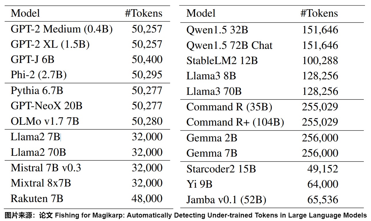
These models were not trained under a controlled comparison. Their different architectures, corpora, control-token reserves, and tokenizer families prevent us from attributing a quality difference to vocabulary size alone.
A larger vocabulary can shorten common strings but allocates more input rows and output classes. A smaller vocabulary concentrates observations into fewer rows while often using more sequence positions for the same text.
Byte fallback inside a subword tokenizer also differs from a model that
processes bytes without learned subwords; we will examine those architectures
in 0x0E.
Counting sequence positions
Let record x contain b(x) UTF-8 bytes and let candidate c emit
n_c(x) model positions. Across a fixed corpus D, the number of input rows
gathered, hidden states processed, and next-token targets is:
Dense attention does not consume a source byte matrix. For independent unpacked records it consumes a logical score area proportional to:
The square is inside the sum because independent records do not attend across their boundaries. Replacing it with would count forbidden cross-record pairs. Packed kernels can avoid materialized padding, but they do not make each record’s legal attention pairs disappear.
For the same 4096-byte input, suppose candidate A emits 1024 IDs and candidate B emits 2048:
positions:         1,024 versus 2,048       -> 2x
logical QK pairs:  1,048,576 versus 4,194,304 -> 4x
bytes per token:   4 versus 2
That is a workload transformation before the first Transformer block runs.
Real latency still depends on layout, batch, kernel, hardware, and phase, so
Q_c is an accounting proxy rather than a throughput claim.
Counting vocabulary parameters and projection work
Let vocabulary width be V, hidden width be d, and let b_o indicate an
output bias. The input table stores:
An untied output matrix stores another Vd; a tied head reuses input-table
storage but still computes a vocabulary-width logit vector. Therefore:
For N hidden positions and the convention that one multiply-accumulate is two
FLOPs, a dense output projection contributes:
FLOPs and logit elements respectively. Weight tying changes persistent storage, not this output width.
At d=4096 and two bytes per parameter, the input table alone is:
V =  32,000: 131,072,000 parameters =  250 MiB
V = 128,000: 524,288,000 parameters = 1000 MiB
The trade is therefore coupled. Increasing V may reduce N_c(D) and
Q_c(D), while increasing P_vocab, F_logits, and the number of rows that
must receive adequate evidence.
Estimating vocabulary size from experiments
Scaling Laws with Vocabulary studies vocabulary size jointly with model size and training compute:
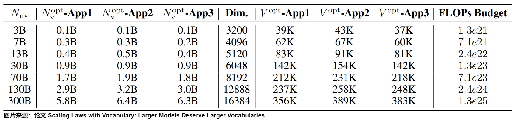
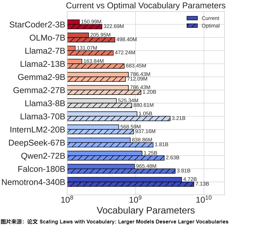
The paper compares three ways to estimate an appropriate vocabulary size:
- IsoFLOPs comparison. Train candidate vocabulary widths under a declared compute budget and compare loss on the same evaluation distribution.
- Derivative-based optimum. Fit or estimate how sequence-side gains and
vocabulary-side cost change with
V, then locate a stationary tradeoff. - Parametric loss fit. Fit a functional form over model size, data/compute, and vocabulary allocation, then predict a minimum within the supported region.
These methods require their paper’s corpus, tokenizer construction, architecture,
compute accounting, fitted range, and evaluation protocol. The reproduced
curves are source-reported, not a rule that a model of a given parameter
count must use one universal V. Extrapolating beyond the fitted range adds
model-form uncertainty.
A useful local abstraction is:
This expression groups the costs that a comparison must account for. Its terms have different units, so an experiment must turn them into explicit constraints or measured objectives before combining them.
0x0C1 Comparing tokenizer candidates
Tokenizer selection is model-component selection. It needs immutable fit, validation, and test roles just as model selection does.
Separating fitting, validation, and test data
fit split:
    learns normalization statistics, merge ranks, piece scores, or vocabulary

validation split:
    applies release gates and chooses one candidate

test split:
    remains sealed until the candidate identity is frozen
Record identity alone is insufficient. Near duplicates, translations, derived
code files, conversation branches, or shards from one document can leak across
roles. The split manifest therefore binds record_id, group_id, split,
slice, exact text bytes, reference counts, deterministic order, and upstream
corpus-release hash. Every group_id must have one split owner.
def validate_split_manifest(records):
    owner = {}
    for record in sorted(records, key=lambda row: row.record_id):
        prior = owner.setdefault(record.group_id, record.split)
        assert prior == record.split
        assert len(record.text.encode("utf-8")) == record.declared_utf8_bytes
        assert len(record.text) == record.declared_codepoints

    assert {record.split for record in records} == {"fit", "validation", "test"}
The tokenizer artifact is fitted only from fit. Validation text may be
encoded by every fitted candidate but cannot change its learned pieces. Test
metrics cannot participate in candidate ordering, threshold tuning, or manual
exception design.
Controlling the comparison
Comparing a 32k BPE artifact with a 128k Unigram artifact changes both family and width. That can be a product comparison, but it is not a one-variable ablation. Declare which dimensions are fixed:
fit-corpus bytes, grouping, sampling, and order
normalization and pre-token boundaries
base alphabet, fallback, and reserved controls
candidate family and deterministic use-time schedule
model hidden width, tying, bias, and parameter dtype
maximum sequence length and truncation policy
evaluation records, slices, templates, and metric estimators
Then vary vocabulary width with nested candidates, or hold width fixed while varying BPE, WordPiece, or Unigram. SentencePiece must be labeled as a framework plus its inner model, not treated as a fourth learning objective.
Computing corpus-level ratios
For sample x, define UTF-8 bytes b(x), normalized codepoints u(x), a
reference-word count w(x) computed independently of the tokenizer, token
count n_c(x), and the number of one-byte final tokens q_c(x). Corpus-level
metrics are:
These are ratios of totals because a corpus-cost question weights each byte, word, or model position once. The macro average
answers a different question: the average record’s ratio, giving a short record the same weight as a long one. Neither estimator is inherently invalid, but publishing one under the other’s name is.
For a tokenizer with UNK, coverage needs a separate rate. Byte fallback can
make UNK rate zero while still producing long sequences. Compression,
coverage, boundary alignment, and downstream quality remain different axes.
Comparing languages and domains
Global totals can conceal allocation inequality. Keep language, script, prose,
code, mathematics, identifiers, numbers, URLs, noisy text, and length bands as
first-class slices. Against baseline candidate r, token amplification for
slice s is:
Because both candidates encode the same records, retain paired per-record deltas as well as aggregate ratios. Report at least:
total tokens, bytes/token, codepoints/token, and fertility
p50, p95, and maximum record length
truncated-record count under the declared maximum
single-byte final-token fraction
sum of legal per-record n(x)^2 attention pairs
per-slice amplification against the baseline
offset reconstruction for span-owned tasks
encode/decode throughput only with pinned runtime and hardware
An overall reduction with A_c,s > 1 on a required slice is a product tradeoff,
not an unqualified improvement.
Evaluating model quality
Primary studies reach the same caution from different directions. Tokenizer Choice for LLM Training: Negligible or Crucial? evaluates tokenizer choice as part of model training rather than as compression alone. Beyond Text Compression argues for evaluation across model scales and tasks. The Chinese Mixtral language-adaptation study tests vocabulary expansion inside a broader continued-training setup; its results are source-reported rather than a guarantee for other models.
Therefore:
fewer tokens       != better task quality
higher bytes/token != better semantic units
zero UNK           != efficient allocation
larger V           != better coverage for every slice
Intrinsic tokenizer gates can reject mechanically bad candidates. A final model choice still needs controlled training or adaptation and downstream evaluation. The small example here does not measure task quality.
Comparing three vocabulary sizes
The executable example binds 12 group-isolated records across prose, code, numbers, and CJK slices. It evaluates three nested byte-BPE candidates. All start with 256 byte rows and eight reserved control rows:
compact-268:
    4 merge rows: th, the, in, ing

balanced-272:
    compact prefix + er, re, ==, 10

expanded-279:
    balanced prefix + fo, foo, ba, bar, partial/full UTF-8 中, xy
The larger candidates preserve every earlier merge rank and ID. This isolates append-only width rather than silently changing old address semantics.
The validation results are:
| Candidate | Validation tokens | P_vocab | Zero direct fit-emission merge rows | Eligibility |
|---|---|---|---|---|
compact-268 | 29 | 17,420 | 2 | pass |
balanced-272 | 25 | 17,680 | 2 | pass and selected |
expanded-279 | 21 | 18,135 | 6 | reject: parameter budget and exposure gate |
The expanded candidate produces the shortest validation sequence. It is rejected because it exceeds the declared parameter and exposure limits. Selection minimizes positions only among candidates that pass these checks:
eligible = []
for candidate in candidates:
    report = evaluate(candidate, fit, validation)
    failures = apply_validation_gates(report)
    if not failures:
        eligible.append(report)

winner = min(
    eligible,
    key=lambda report: (
        report.validation_tokens,
        report.vocabulary_parameters,
        report.candidate_id,
    ),
)

assert test_metrics_consulted_during_selection is False
The final tie-break makes selection independent of candidate list order. The candidate set itself is hashed from sorted semantic hashes; file order cannot secretly choose the winner.
The checks must include exact reconstruction: decoding each candidate’s IDs
has to return every validation byte string unchanged. Otherwise a candidate
that maps unusual text to an unknown token could produce fewer tokens and win.
The three candidates here are byte-level BPE with 256 byte rows and no
normalization, so they reconstruct every input by construction; a vocabulary
with an [UNK] fallback does not.
Comparing parameter and computation costs
The synthetic model contract uses d=64, two-byte parameters, tied
input/output storage, and an output bias. Thus:
and for N validation positions:
| Candidate | Positions N | Pair proxy Q | Logit elements NV | Projection FLOPs | Resident vocabulary bytes |
|---|---|---|---|---|---|
compact-268 | 29 | 325 | 7,772 | 994,816 | 34,840 |
balanced-272 | 25 | 243 | 6,800 | 870,400 | 35,360 |
expanded-279 | 21 | 203 | 5,859 | 749,952 | 36,270 |
Although the expanded candidate reduces sequence work in this small example, it exceeds the release limits. These calculated counts explain the selection; they are not measured tokenizer or GPU performance.
Measuring how vocabulary rows are used
The fit diagnostic counts final emitted merge IDs. It does not equate a zero count with structural impossibility:
ID 264 = "th": zero final emissions in the fit records,
               but encode("th") emits [264]

ID 267 = "ing": zero final emissions in the fit records,
                but encode("ing") emits [267]
A later merge may consume these rows as intermediate pieces, leaving them absent from the final encoding. To interpret their counts, separate the following measurements.
Direct exposure counts how often an ID appears in the final encoded training corpus. Reachability asks whether any permitted input can emit it at all. Neither measure tells us how the model learned the corresponding row.
For that, count positive next-token targets and input-embedding lookups, and consider the gradients received by output rows both as targets and as competing softmax classes. Behavioral undertraining requires model probes that reveal anomalous probabilities or generated text.
Fishing for Magikarp supplies a method for detecting undertrained tokens in trained models. A raw frequency threshold is only a screening diagnostic; row norm alone and zero direct corpus emissions do not prove the paper’s behavioral condition.
Reporting the held-out test result
After selecting balanced-272, the experiment evaluates the test split and
reports 27 positions across three records. That number describes the selected
candidate; it cannot revise the selection. If test evidence triggers a release
concern, the experiment is failed or a new versioned experiment begins. The
same test set must not be used to adjust the acceptance criteria.
0x0C2 Updating a model vocabulary
Selecting a tokenizer candidate does not make it checkpoint-compatible. A vocabulary transition changes an address space and every tensor or cache keyed by that space.
Appending vocabulary entries
The example migrates from compact-268 to balanced-272. IDs 0..267 keep
their old byte pieces and merge ranks; IDs 268..271 are appended. The tensor
shapes become:
input embedding:   [268,64] -> [272,64]
output bias:       [268]    -> [272]
tied output head:  reuses the resized input-table storage
With Delta V = 4, the new trainable state is:
For two optimizer slot tensors per trainable scalar, the optimizer gains
2 * 260 = 520 slot values in addition to parameter gradients and any master
weights required by the training recipe.
Append-only identity protects old standalone IDs. It does not guarantee that old text keeps the same segmentation: a new higher-rank continuation can combine old pieces into a newly appended ID. Encoded datasets and prefix caches must be recomputed against the new semantic artifact.
Initializing new rows
The synthetic migration initializes each appended input row from its immediate old decomposition:
ID 268 "er" <- mean(E[101], E[114])
ID 269 "re" <- mean(E[114], E[101])
ID 270 "==" <- mean(E[61],  E[61])
ID 271 "10" <- mean(E[49],  E[48])
This preserves dimensions and gives each row a composition-based starting point. It does not teach contextual meaning or calibrate the new output class. Other defensible policies answer different questions:
Random initialization at the old table’s scale is simple but starts without piece-specific information. Using the old rows’ mean and covariance can limit initial logit disruption under a stated model, though it also ignores the new piece’s decomposition.
A mean or weighted sum of the old pieces supplies a piece-specific starting point, but inherits any weaknesses in those rows and does not capture context. A learned projection or adapter can use continued-training data to align new rows to a language or domain, at the cost of additional training and implementation choices.
The
Empirical Comparison of Vocabulary Expansion and Initialization Approaches
compares such choices under its own languages, models, tasks, and training
contracts; the results are source-reported rather than universal. Official APIs
such as Hugging Face
resize_token_embeddings
expose concrete resizing and initialization behavior, including
version-specific mean-resizing options, and retie weights after resizing. A
release must record the pinned library version and observed tensor behavior
rather than assuming every implementation follows this example.
Resizing model and optimizer tensors
def migrate_append_only(model, optimizer, old_tokenizer, new_tokenizer, plan):
    old_v = model.get_input_embeddings().weight.shape[0]
    new_v = new_tokenizer.model_vocab_size

    assert old_v == 268
    assert new_v == 272
    assert new_tokenizer.semantic_prefix(0, old_v) == \
           old_tokenizer.semantic_prefix(0, old_v)

    model.resize_token_embeddings(new_v)
    embedding = model.get_input_embeddings().weight
    output = model.get_output_embeddings()

    for row in plan.new_row_initialization:
        assert row.new_id >= old_v
        assert all(source_id < old_v for source_id in row.source_old_ids)
        embedding[row.new_id] = embedding[row.source_old_ids].mean(dim=0)

    if model.config.tie_word_embeddings:
        model.tie_weights()
        assert output.weight.data_ptr() == embedding.data_ptr()
    else:
        initialize_untied_output_rows(output.weight, plan)

    model.get_output_embeddings().bias[old_v:new_v].zero_()
    expand_optimizer_state_by_parameter_identity(optimizer, model, old_v, new_v)
    return model, optimizer
The sketch deliberately names unresolved choices. An untied output head needs
its own row policy. Some models have no output bias. Optimizers may store
momentum, variance, master weights, factorized state, or sharded state. A generic
resize call cannot infer those contracts.
Updating dependent data and model state
A coordinated transition must account for:
tokenizer semantic and release hashes
input table, output head, bias, and tied alias
optimizer and gradient/master state
vocabulary-axis shard ownership and checkpoint metadata
quantization groups, scales, codebooks, and calibration artifacts
tokenizer-derived train/validation/test datasets
chat-template and special-token golden cases
prefix, prompt, tokenization, and compiled-graph caches
serving admission rules and rollback target
Quantized rows cannot simply be appended to an arbitrary group without checking
the representation contract. Vocabulary-sharded tables may cross partition
boundaries when V changes. Re-encoding can alter sequence length, truncation,
packing, label positions, and dataset shard sizes even when every old ID remains
valid.
Initialization is not a substitute for continued training. The migration plan requires adaptation after rows are appended, with the new tokenizer active for the training data and with evaluation covering old and new behavior.
Deciding what can be reused
Not every changed file implies the same migration. Classify the transition before deciding whether to reuse, rebuild, adapt, or reject:
A byte-identical redeploy keeps the release and bundle hashes unchanged and needs ordinary integrity checks. A repackage can change file bytes while preserving behavior; reusing IDs and model rows then requires the reconstructed semantic hash and golden cases to agree.
A template-only change keeps tokenizer semantics but changes the sequence format. Rebuild template-derived data and caches and evaluate the model’s compatibility with that format. Appending vocabulary entries also requires a verified old-ID prefix, initialized new rows, resized model state, re-encoded data, adaptation, and a coordinated release.
If neither equivalence nor a complete row mapping can be established, treat the replacement as incompatible. Existing datasets and checkpoints cannot be reused without an explicit migration or retraining plan.
Matching width, successful deserialization, or plausible decoded text proves none of these classes. Reconciliation must compare semantic declarations and golden behavior at the layer where reuse is claimed.
Releasing and restoring a complete version
Publish one immutable bundle revision:
stage candidate tokenizer and semantic manifest
    -> verify append-only old-ID prefix
    -> resize and initialize model tensors
    -> expand or rebuild optimizer/shard/quantization state
    -> re-encode tokenizer-derived datasets
    -> rerun byte reconstruction and sequence golden cases
    -> train/adapt and evaluate old plus new slices
    -> invalidate identity-keyed runtime caches
    -> publish one complete bundle
    -> atomically switch admission

on failure:
    stop admitting the new bundle
    discard caches keyed by its tokenizer/template identity
    restore compact-268 with its matching checkpoint and datasets
    never combine one revision's tokenizer with another revision's rows
Deploying files individually can pair a valid tokenizer with the wrong model or dataset. Release them together, and restore the same complete set when rolling back. These release examples assume the switch from one bundle to the next is atomic, so that no request sees parts of both; they do not show how a storage system or a serving fleet provides that guarantee.
Testing a release on a small workload
First check that hashes, old-ID mappings, model rows, dataset bindings, and cache namespaces agree. Then evaluate whether the release preserves the old workload and improves the cases that motivated the change.
Let one release bundle be the ordered state
These components must be staged, tested, promoted, and restored together. The structural checks are:
One false term rejects the candidate. Averaging these checks into a score would allow a perfect compression result to hide a checkpoint-tokenizer mismatch.
Only a mechanically admitted bundle may receive canary traffic. The lifecycle
compatibility example routes 500 basis points, or 5%, into the isolated
cache-expanded-272-r18 namespace: the cache of release r18, which replaces
compact-268 (release r17) with the 272-row vocabulary called
balanced-272 above. The example evaluates three deliberately different
slices:
The 40 old-behavior cases reach a maximum relative length of 1.04, below
their 1.10 limit. The 24 new-piece cases reach 0.88 against the same limit.
The eight control-and-stop cases stay at 1.00, exactly their allowed ratio.
All three groups have zero stop mismatches and zero cache-namespace mismatches.
For this synthetic contract, promotion requires
Here rho_s is the largest measured candidate-to-stable length ratio in slice
s, and tau_s is that slice’s declared limit. These thresholds are synthetic
test data, not recommended production tolerances. Before production use, we
would also evaluate task quality, latency, memory, safety, and any other
requirements of the workload.
The state transition is intentionally asymmetric:
def admit_candidate(stable, candidate, canary):
    require(candidate.cache_namespace != stable.cache_namespace)
    require_mechanical_reconciliation(stable, candidate)

    result = run_canary(candidate, traffic_basis_points=500)
    if not result.every_declared_slice_passed:
        stop_admission(candidate.bundle_id)
        invalidate(candidate.cache_namespace)
        restore_atomic_bundle(stable)
        return "rolled_back"

    promote_atomic_bundle(candidate)
    return "promoted"
Rollback does not reverse the candidate in place. It routes new requests to the previous saved bundle, restores all six bound component identities, and invalidates only the candidate cache namespace. Stable caches must not be invalidated accidentally; candidate caches must not survive to contaminate a later release with the same visible prompt.
0x0D Requests, streaming, and stopping
The tokenizer does not disappear after it returns input_ids. At runtime its
artifacts meet four other state machines:
sequence compiler:
    messages + mode -> exact prompt IDs + prompt boundary

input transport:
    byte chunks -> provisional tokenizer state -> stable committed IDs

prefix reuse:
    exact model-state identity + stable ID blocks -> cache admission decision

output transport:
    sampled IDs -> token bytes -> valid text -> stop-safe client output
These stages advance at different times. Received bytes may still change an earlier tokenization. Stable prompt IDs may occupy an incomplete cache block. Generated IDs may contain only part of a UTF-8 character, and valid text may still be the beginning of a stop string. Each stage must wait until its output is safe for the next stage to use.
Encoding a request before caching
The runtime begins with the outer grammar, not with visible message text. The
official Hugging Face chat-template
documentation
illustrates why: different model families expect different control tokens, and
add_generation_prompt can append an assistant-start marker that is absent
from the visible messages. If a template has already inserted controls,
tokenizing the resulting string with another automatic special-token layer can
duplicate them. continue_final_message is another entry mode, not a synonym
for adding a generation prompt.
The runtime compiler therefore consumes pinned artifacts and returns an exact sequence object:
@dataclass(frozen=True)
class CompiledRequest:
    input_ids: tuple[int, ...]
    prompt_boundary: int
    special_tokens_mask: tuple[int, ...]
    sequence_ownership: tuple[str, ...]
    tokenizer_semantic_hash: str
    template_hash: str

def compile_request(messages, mode, tokenizer, template, checkpoint):
    require(tokenizer.semantic_hash == checkpoint.tokenizer_semantic_hash)
    require(template.hash == checkpoint.template_hash)

    compiled = template.compile(messages, mode=mode, tokenizer=tokenizer)
    require(compiled.prompt_boundary == len(compiled.input_ids))
    require(all(0 <= i < checkpoint.vocab_size for i in compiled.input_ids))
    require_aligned(compiled)
    return compiled
The runtime example uses the saved assistant_prefill result from the
conversation-formatting example. That formatter emits exactly sixty IDs and
sets prompt_boundary = 60. The runtime example does not rebuild the template
from message strings. It verifies the sequence-bundle hash, case identity,
complete ordered ID list, and boundary before constructing a runtime identity.
Choosing the cache identity
Choose the hash inputs according to what the cache needs to identify.
The visible request consists of messages, client options, and request metadata. Sequence provenance additionally records the tokenizer, template, and entry mode that produced the input. The encoded sequence itself is the exact ordered IDs plus their aligned metadata.
Cache reuse asks about model state. Its identity includes the model revision, any adapter that changes cached states, positions, extra model inputs, and the exact ID prefix. Equal visible requests do not establish equality at these later stages.
Visible strings are insufficient. Different control IDs can be hidden by decoding, and two tokenizations can reconstruct the same bytes. Conversely, if two upstream compiler releases produce exactly the same admitted IDs, the tokenizer and template names are not necessarily required to describe the mathematical model state. This creates a legitimate design choice:
minimal model-state key:
    model revision
    adapter identity when it changes projected state
    position/context policy
    extra model-input identity
    exact ordered token IDs

conservative release/provenance key:
    every minimal field
    + tokenizer semantic identity
    + template identity
The minimal key can reuse more prefixes after a compiler-only migration that provably emits identical IDs. The conservative key makes release isolation and incident rollback simpler, at the cost of fewer hits. Neither policy justifies keying on decoded text. The key policy is itself versioned runtime state.
Adapters need the same precision. If an adapter changes hidden states used to produce cached keys and values, its identity belongs in the key. A runtime may prove that a particular later-only transformation does not affect the cached state, but that proof is architecture and engine specific. “An adapter is small” is not such a proof.
Linking cache blocks to their prefixes
Suppose a compiled prompt has length and a cache admits blocks of tokens. The number of complete admissible blocks and the request-owned tail are
The floor appears because only complete blocks enter the cache in this example, following the cited version of the vLLM prefix-caching design document used as an implementation comparison. That document describes a block hash derived from the parent hash, exact block token IDs, and extra identity fields such as LoRA and multimodal inputs; it also explains why only full blocks are cached in that design. Other releases or engines can use different layouts.
Let denote the pinned state-changing identity fields and let be the exact IDs in block . A parent chain is
The parent hash is necessary because a block containing IDs [a,b,c] after
one prefix is not the same autoregressive state as the same IDs after another
prefix. If block changes, then changes and every descendant key
changes through the recurrence. This gives prefix reuse rather
than unordered block reuse.
def cache_blocks(request, block_size, key_mode):
    parent = ROOT
    blocks = []
    full_count = len(request.input_ids) // block_size

    for i in range(full_count):
        ids = request.input_ids[i * block_size : (i + 1) * block_size]
        payload = model_state_fields(request, mode=key_mode)
        payload.update(parent_block_hash=parent, block_token_ids=ids)
        parent = framed_sha256("prefix-cache-block-v1", payload)
        blocks.append((i, ids, parent))

    tail = request.input_ids[full_count * block_size :]
    return blocks, tail  # tail is not globally admitted by this policy
For the sixty-ID prompt and ,
Seven complete blocks can enter the cache. IDs 56..59 remain in an
incomplete block used only by this request.
The cache checks give the following results:
| Probe | Minimal key hits | Conservative key hits | Reason |
|---|---|---|---|
| identical request | 7/7 | 7/7 | every key input is equal |
| token at position 18 changes | 2/7 | 2/7 | blocks 0 and 1 precede the changed third block |
| same IDs, different template provenance | 7/7 | 0/7 | model state is equal under the minimal contract; release identity is not |
| same IDs, different tokenizer provenance | 7/7 | 0/7 | same distinction |
| model, adapter, position, or extra input changes | 0/7 | 0/7 | state-changing identity differs at the root |
These probes use constructed requests, so the hit counts are not a workload benchmark. Nor does this section measure tokenizer latency, serving throughput, or a particular engine release; such measurements need a fixed model, tokenizer, template, runtime, hardware, workload, and scheduler. The cited vLLM version also documents hash collisions and an optional SHA-256 mode. This example uses framed SHA-256 to distinguish fields and object types; the runtime still needs a policy for checking stored payloads and handling collisions.
Passing stable input IDs to the model
The network can split input at any byte, including inside a character or a
piece the tokenizer would otherwise keep together. We can see this with the
UTF-8 bytes for €:
transport chunks:          e2 | 82 | ac
provisional ranked-BPE:   [226] [260] [260,172]
committed emissions:        []    []   [260,172]
The first chunk is not valid standalone UTF-8, and the second chunk changes the
provisional tokenization. In this example, the third chunk completes the unit
being encoded, so no later input can change [260,172]. To decide which IDs
are ready for the model, we track progress at four stages:
bytes received:
    all bytes delivered by the network

bytes decoded:
    the portion decoded into complete units by the input codec

token IDs finalized:
    IDs that subsequent input cannot change under the chosen encoding rules

token IDs accepted by the model:
    finalized IDs used for model computation or cache reuse
The runtime can accept only IDs that the tokenizer has finalized.
class StreamingInput:
    undecided_bytes: bytearray
    committed_ids: list[int]

    def push(self, transport_chunk, declared_unit_boundary=False):
        self.undecided_bytes.extend(transport_chunk)
        provisional = tokenizer.encode_unit(bytes(self.undecided_bytes))

        if not declared_unit_boundary:
            return StableEmission(ids=(), provisional_ids=tuple(provisional))

        self.committed_ids.extend(provisional)
        self.undecided_bytes.clear()
        return StableEmission(ids=tuple(provisional), provisional_ids=tuple(provisional))
Buffering to a known boundary adds latency and memory use. Suffix retokenization or an incremental algorithm can emit earlier, but must reproduce batch encoding and support the same restart behavior. A guessed suffix length is insufficient.
The OpenAI tiktoken core API
exposes encode_with_unstable, returning a stable prefix and possible
completions. Its docstring marks the API as unstable, so integration depends
on the chosen library version.
On cancellation, discard pending tokenizer state, incomplete UTF-8 bytes, and any work scheduled for uncommitted IDs:
def cancel_input(stream, runtime_request):
    stream.undecided_bytes.clear()
    stream.provisional_ids.clear()
    runtime_request.discard_uncommitted_model_work()
    # Already admitted stable cache blocks follow M5 ownership and policy.
In the synthetic trace, cancellation after chunks e2 | 82 leaves zero
committed IDs. The undecided bytes, provisional IDs, and uncommitted model work
all become empty. Caching [226] or [260] before finalization would attach
model state to an encoding that the third byte invalidates.
Decoding output incrementally
Generation reverses the direction but not the need for boundaries. A token ID
maps to bytes first. Those bytes may be only part of a UTF-8 scalar. The
tiktoken API exposes decode_single_token_bytes for this reason and warns
that decoding a single token directly to text can be lossy when its bytes do
not form valid UTF-8.
The safe output path is
sampled IDs
    -> exact piece bytes
    -> incremental UTF-8 decoder
    -> stop-prefix holdback
    -> client-visible text
not
each token ID -> standalone text -> concatenate strings
Suppose synthetic token 401 emits byte e2 and token 402 emits bytes
82 ac. Decoding 401 alone must not insert a replacement character. The
incremental decoder buffers e2; after 402, it consumes e2 82 ac and emits
€ once. This is a codec-state transition, not a token-boundary property.
decoder = codecs.getincrementaldecoder("utf-8")("strict")

for token_id in generated_ids:
    piece_bytes = decode_single_token_bytes(token_id)
    text_delta = decoder.decode(piece_bytes, final=False)
Replacement decoding is a separately declared lossy API policy. It cannot be used internally and later advertised as byte-exact reconstruction.
Specifying when generation stops
“Stop on STOP” is underspecified. A runtime can stop on:
one control ID:
    EOS or EOT

one exact ID sequence:
    [83, 84, 79, 80]

one text/byte string across arbitrary token boundaries:
    "STOP", perhaps emitted as [403, 79, 80]

one external budget or signal:
    maximum generated IDs, cancellation, deadline, or policy event
The official Hugging Face
StopStringCriteria
documents a tokenizer-aware stop-string criterion. Its implementation
source
precomputes token overlap information so a stop can be recognized across token
boundaries and with token overhang. That is an implementation contract, not
proof that a naive decoded-substring search has the same behavior.
Record the following fields before generation begins:
@dataclass(frozen=True)
class StopPolicy:
    single_token_ids: frozenset[int]
    multi_token_sequences: tuple[tuple[int, ...], ...]
    text_stop_strings: tuple[str, ...]
    match_scope: Literal["generated_suffix_after_prompt_boundary"]
    strip_matched_stop: bool
    max_new_tokens: int
The match scope starts with an empty generated suffix at prompt_boundary.
Prompt tokens do not seed the matcher. Otherwise a stop-looking sequence inside
the system prompt or user content could terminate generation before one token
is sampled.
Token-sequence and text-string policies are not interchangeable. Exact ID matching is unambiguous for a pinned tokenizer but misses alternate segmentations of the same bytes. Text matching catches alternate segmentation, but it needs an exact codec, normalization, case, and boundary policy. A production API must say which one it means.
Holding back a possible stop string
If a matched stop must be stripped, the runtime cannot optimistically expose every valid text fragment. The beginning of a stop may already have been sent to a client that cannot retract output.
Let be the configured stop patterns encoded as exact bytes, and let be the currently uncommitted output-byte suffix. Define
Why retain the longest proper prefix? Any shorter candidate is contained in that suffix, while emitting one byte from the longest candidate could destroy a future full match. If no complete stop string ends at the current output position, bytes before the final bytes are stop-safe. They are client-safe only after the UTF-8 decoder also confirms a complete text boundary.
For pattern STOP:
pending suffix "S"    -> h=1 -> emit nothing
pending suffix "ST"   -> h=2 -> emit nothing
pending suffix "STO"  -> h=3 -> emit nothing
pending suffix "STOP" -> full match -> strip pattern and finish
Buffering the entire response also preserves stripping semantics, but destroys streaming latency. Optimistically emitting and later retracting can work only when the client protocol explicitly supports retractions. Prefix holdback is the bounded middle ground; with straightforward matching it retains at most stop bytes, in addition to the UTF-8 decoder’s own incomplete-scalar state.
The output examples cover five cases:
With synthetic IDs [400,401,402,260], the split UTF-8 bytes form OK € and
control ID 260 stops generation without appearing in the output.
For [400,83,84,79,80,33], an exact-ID stop [83,84,79,80] leaves OK ;
the later 33 is unprocessed. The alternate segmentation
[400,403,79,80,33] produces the same stop text, but its [403,79,80] IDs
do not match that ID pattern. A text stop still recognizes STOP.
A budget of three generated IDs applied to [400,65,66,67] leaves OK AB
and does not process 67. With [400,33] and no stop, the synthetic source
simply runs out after producing OK !.
The example’s token bytes are deliberately synthetic. They test the state machine, not a production vocabulary. The exact-ID and alternate-segmentation cases prove why both token and text policies may be needed. The EOT case proves that a control ID can terminate without contributing ordinary output bytes.
Tracking hidden stop tokens and cancellation
After a stripped stop, three records can differ:
client-visible text:
    bytes proven UTF-8-valid and stop-safe

generated-token record:
    IDs sampled and inspected, including an ID or sequence that triggered stop

model/KV state:
    positions whose state has been validly computed and committed by M3.10/M5
A token hidden from the client can still appear in generation diagnostics or have associated model state. Conversely, a correction sent to the client does not establish matching cached state. The generation loop must track these states separately when appending, stopping, or rolling back.
This boundary also prevents a subtle category error during cancellation:
def finish_output(result, stop_policy):
    return OutputResult(
        visible_text=result.stop_safe_text,
        processed_generated_ids=result.generated_ids,
        finish_reason=result.finish_reason,
        matched_stop=result.matched_stop,
        # No claim about KV commit is derived here.
    )
0x0E Models that process bytes and characters
A model can start from bytes or characters and reduce the sequence inside the network. Some architectures process every raw position; others form fixed patches, learn mixtures of short blocks, or choose boundaries from context.
The location of this reduction affects training targets, position counts, causality, generation, and cache state. We will follow where each architecture compresses the sequence and which operations still process the raw units.
The following descriptions follow the ByT5, CANINE, Charformer, MEGABYTE, and BLT papers. The small numerical example compares their position counts, not their quality or throughput.
Counting bytes, characters, and patches
Let one record contain n_b UTF-8 bytes and n_c Unicode code points. Define:
n_raw       positions at the architecture's external input coordinate
n_local     position counts consumed by lightweight/local stages
n_global    positions consumed by the expensive global stack
n_output    positions exposed or generated at the external output coordinate
The coordinates matter. For the string A naïve cat.\n:
UTF-8 bytes:
    41 20 6e 61 c3 af 76 65 20 63 61 74 2e 0a
    n_b = 14

Unicode code points:
    A, space, n, a, ï, v, e, space, c, a, t, ., newline
    n_c = 13
Here n_b != n_c because ï occupies two UTF-8 bytes but one Unicode code
point. A sequence-length comparison must state which unit it counts.
For a fixed reduction width r, the global length is
For variable patches with half-open intervals
[q_j,q_{j+1}), it is instead
To turn these lengths into FLOP estimates, we would also need the local and global widths and depths, cross-attention, output projections, and generation schedule.

CANINE is an encoder; the ByT5 and Charformer papers use encoder-decoder setups; MEGABYTE and BLT generate bytes autoregressively. Their global position counts therefore describe different computations.
ByT5: processing bytes directly
ByT5 asks how far a standard T5 architecture can go with minimal change. It UTF-8 encodes text, maps the 256 possible byte values to rows, retains explicit control IDs, and applies the main Transformer directly to byte positions. There is no learned subword lexicon and no pre-global downsampler:
Therefore:
The byte alphabet reduces input and output table size. Longer sequences, however, increase attention, feed-forward, and autoregressive decoding work. Parameter count, training FLOPs, and inference speed must be measured separately.
The released paper contract also changes training and capacity allocation, not only input IDs:
input unit:
    UTF-8 bytes; illegal output-byte handling is an explicit decoder policy

pre-training:
    span corruption over byte spans, with longer source-reported mean spans
    than the subword mT5 baseline

architecture:
    an encoder three times as deep as the decoder in the reported ByT5 design

generation:
    one autoregressive output decision per generated byte
Those choices are coupled. Copying a 256-row embedding table into an unrelated decoder-only model would not reproduce ByT5.
CANINE: reducing and restoring character positions
CANINE’s public interface begins from Unicode code-point integers rather than
UTF-8 bytes. It avoids one embedding row per Unicode scalar by applying several
hash functions and concatenating their learned lookup results. For code point
x_i, the paper’s construction can be summarized as
Collisions in one table are tolerated; multiple independent hash projections make identical complete collisions less likely. Hash identity and table count are checkpoint state, not replaceable implementation trivia.
The sequence graph is:
For sequence-level character outputs, each reduced state is repeated across its
r source positions, concatenated with local character features, convolved,
and passed through a final Transformer layer:
The source-reported configuration uses local blocks of 128 characters, stride
r=4, and reduces 2,048 character positions to 512 deep-stack positions. The
paper then restores character-aligned representations for sequence tasks.
CANINE input:
    code-point IDs [B, n_c]

after local encoder:
    h_init [B, n_c, d]

after stride-r convolution:
    h_down [B, ceil(n_c / r), d]

after task-facing upsampling:
    y_seq [B, n_c, d]
CANINE-C and CANINE-S also use different pre-training target construction: one predicts characters without subword targets; the other may use subword information as a soft training signal while keeping code points as model inputs. That distinction prevents the slogan “tokenization-free” from hiding training-time dependencies.
CANINE’s character-aligned outputs support classification and sequence prediction. They do not by themselves define an autoregressive generation loop.
Charformer: learning block representations
Charformer introduces Gradient-Based Subword Tokenization (GBST). Let
X in R^(L x d) be byte or character embeddings. For each candidate block
width b <= M, a pooling function forms strided block representations:
The paper uses stride b, optionally precedes enumeration with a 1-D
convolution, and realigns each block sequence to length L by repeating block
representations over their covered positions. A scoring network produces
Each position receives a differentiable mixture, not one committed piece:
Only afterward does a separate fixed-rate mean pool reduce sequence length:
The scoring network changes the representation at each position through a differentiable mixture. It emits neither a vocabulary ID sequence nor a hard segmentation.
learned:
    which block sizes contribute to each position's latent representation

fixed by configuration:
    the final downsampling rate d_s and therefore the global sequence length

not produced:
    a portable list of discrete token IDs or a hard segmentation boundary list
The paper compares offsets against a pre-GBST convolution, optionally calibrates scores across positions, and reports task-dependent choices about freezing GBST during fine-tuning. These are training and implementation variants, not merely different vocabulary files.
The same details constrain generation. A convolution that reads both sides of a position, or score calibration through all-position interactions, cannot be silently reused as an online causal patcher. Charformer’s paper establishes a learned input representation for its evaluated encoder-decoder setup; it does not by itself prove a stable discrete segmentation for arbitrary streaming autoregressive decoding.
MEGABYTE: predicting bytes within fixed patches
MEGABYTE reshapes a byte sequence of length T into K=ceil(T/P) fixed
patches of width P. The global Transformer runs across patches, while a
smaller local Transformer predicts bytes inside each patch.
The causal shift is the crucial implementation detail. Global input patch k
contains the previous byte patch, not the patch it will help predict:
The global output is split into P slices. Local row p receives the
corresponding global slice plus the previous byte embedding:
with a learned local pad at p=0. Tensor shapes are:
bytes:
    x                [B, K, P]

global patch input:
    h_global_in      [B, K, P * D_G]

split global context:
    context          [B, K, P, D_G]

local byte states:
    h_local          [B, K, P, D_L]

byte logits:
    logits           [B, K, P, 256]
The local factorization is not optional if the model must represent arbitrary within-patch dependence:
A single categorical distribution over a whole patch would need 256^P
outcomes. Independent per-position predictions would be tractable but could not
represent correlations such as a patch being either cat or dog without
also assigning mass to mixed strings. The autoregressive local model supplies
that conditional dependence.
The two-level attention-shape derivation is
For feed-forward-dominated models, the paper approximates forward computation as
where m_G and m_L are global and local non-embedding parameters. This is a
paper-level approximation, not a measured kernel model.
MEGABYTE also studies causal convolutions before patching, cross-patch local attention, and strided inference. Strided inference spends an extra shifted forward pass to use earlier within-patch positions; it is a quality/cost alternative, not a free correction to fixed boundaries.
BLT: choosing patch boundaries dynamically
BLT accepts bytes and supports several patching strategies, including fixed stride, BPE-shaped groups, whitespace boundaries, and entropy-based boundaries:

These variants allocate global work differently:
fixed stride:
    predictable count and layout; boundaries ignore content

space-like rule:
    spends a global step near selected lexical boundaries; language/domain bias

global entropy threshold:
    starts a patch where next-byte uncertainty exceeds theta_g

relative entropy jump:
    starts a patch where H_i - H_(i-1) exceeds theta_r
For a causal byte predictor p_e, conventional next-byte entropy is
The indexing policy must be explicit: the synthetic trace below treats a high-entropy byte as the first byte of a new patch. Another implementation may record the same boundary as the end of the preceding half-open interval.
Keeping patch boundaries stable during generation
At generation time, future bytes do not exist. If f_p returns boundaries,
then committed boundaries before position i must be prefix stable:
Offline BPE does not satisfy this in general. Consider ranks
rank 0: b + c -> bc
rank 1: a + b -> ab
The complete prefix ab becomes [ab]. After appending c, the higher-priority
b+c merge produces [a,bc]; the former boundary at byte 2 disappears inside
a piece crossing the prefix cut. The segmentation was valid offline, but it was
not safe to commit while generating.
Entropy patching can satisfy the invariant only when H_i depends on bytes
available before decision i and the entropy model’s state is replayed
identically in training and generation. An offline entropy table computed with
future context would not become causal merely because its values are called
entropy. The synthetic entropy starts used in the comparison below,
[0,2,4,8,9,13], are prefix stable: each start compares one next-byte
entropy, computed from earlier bytes only, with a single fixed threshold, so
appending bytes never moves an earlier start.
Connecting local byte states and global patch states
BLT consists of a lightweight local byte encoder, a large latent global Transformer over patch states, and a lightweight local byte decoder:
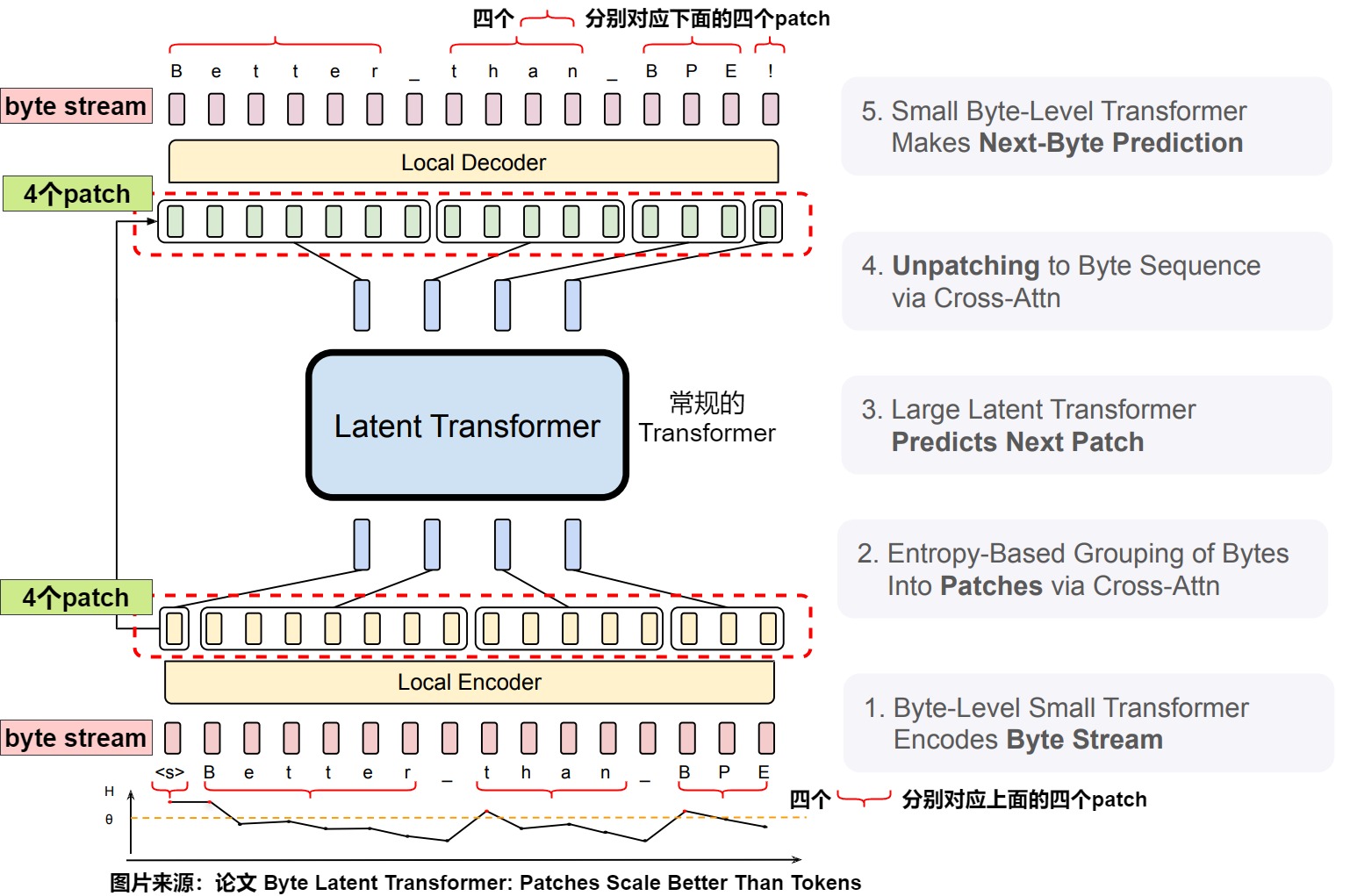
The encoder can augment byte embeddings with hashed byte n-grams. For trailing
n-gram g_(i,n)=(b_(i-n+1),...,b_i):
Local causal Transformer layers build byte states. Patch queries then attend only to byte rows belonging to their patch, producing inputs for the block- causal global Transformer. The decoder reverses the cross-attention direction: byte states query global patch outputs and then pass through local causal Transformer layers.
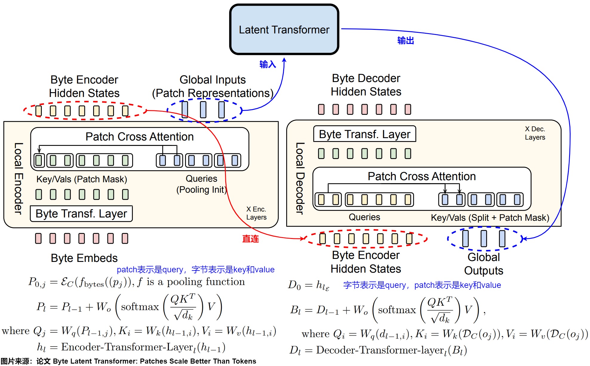
That yields three independently relevant state classes:
patcher state:
    entropy-model state, threshold/rule, current boundary and open patch

global state:
    one latent state and its attention/KV history per completed/current patch

local state:
    byte encoder/decoder history and patch-restricted cross-attention metadata
Patches do not delete byte work. They move most model capacity to fewer global positions while retaining local byte processing and byte-by-byte output. The BLT paper’s FLOP-controlled scaling and robustness results are source-reported under its models, data, patch sizes, and implementation; they are not a universal proof that dynamic patching beats a fixed tokenizer.
Comparing positions for the same sentence
Apply the five declared contracts to the same 14 UTF-8 bytes / 13 code
points. The example uses CANINE stride 4, Charformer downsample rate 2,
MEGABYTE patch width 4, and synthetic BLT entropy starts
[0,2,4,8,9,13] plus final boundary 14.
| Contract | n_raw coordinate | local position state | n_global | n_output | boundaries or reduction |
|---|---|---|---|---|---|
| ByT5 | 14 bytes | no separate local reducer | 14 | 14 bytes | every byte is global |
| CANINE | 13 code points | 13 pre-downsample + 13 post-upsample rows | 4 | 13 aligned states | [0,4,8,12,13] |
| Charformer | 14 bytes | 30 candidate blocks, 14 realigned mixtures | 7 | task dependent | fixed pool groups of 2 |
| MEGABYTE | 14 bytes | 14 local AR rows | 4 | 14 bytes | [0,4,8,12,14] |
| BLT entropy | 14 bytes | 14 encoder + 14 decoder byte rows | 6 | 14 bytes | [0,2,4,8,9,13,14] |
The Charformer candidate total is derived from the example’s padded strided
enumeration for widths 1..4:
As a shape-only diagnostic, n_global^2 is respectively 196, 16, 49,
16, and 36. Those values are not comparable total FLOPs: model widths,
depths, local stages, attention topology, and output serialization differ.
Reproducing the model configuration
The methods also require different release artifacts:
Reproducing ByT5 requires its byte/control IDs, byte-span corruption, and encoder/decoder allocation. CANINE additionally fixes hash tables, local blocks, stride, pre-training targets, and the mapping back to character positions. Charformer needs the candidate widths, scoring network, convolution or offset policy, pooling rate, and task-specific decoder.
MEGABYTE fixes patch width, local/global dimensions, causal shifts, and both levels of cached state. BLT also needs the patcher or entropy model, thresholds, n-gram hashes, and incremental boundary state. These configurations determine the computation that trained the weights and must be reproduced at runtime.
Three other recent methods change what a token stands for, or replace tokens, rather than how text is split. TokenFormer treats model parameters as tokens that input tokens attend to. Large Concept Models predict the next sentence embedding rather than the next token, and FAST turns continuous robot actions into discrete tokens with a discrete cosine transform and compression. Treating them as text-tokenizer variants would hide what their models compute and which kind of input they handle.
0x0F Testing a tokenizer
A tokenizer release should carry a golden corpus containing at least:
empty string and pure whitespace
leading/trailing whitespace and repeated newlines
ASCII, composed/decomposed Unicode, emoji, combining marks
multiple scripts and mixed-script text
numbers, decimal punctuation, long digit runs
code indentation, identifiers, and long no-whitespace spans
literal text that resembles every special token
very long inputs across internal chunk boundaries
For every case, store or verify:
normalized text where exposed
pieces/bytes
input IDs
decoded text
offsets and their coordinate system
special-token mask and sequence IDs
behavior under BOS/EOS/template policy
Useful properties include:
def test_tokenizer_contract(tok, golden_cases):
    for case in golden_cases:
        encoded = tok.encode_structured(case.text, **case.policy)
        assert encoded.input_ids == case.expected_ids
        assert tok.decode(encoded.input_ids) == case.expected_normalized_text
        encoded.validate(tok.vocab_size)

        for token_id in encoded.input_ids:
            assert 0 <= token_id < tok.vocab_size

def test_disallowed_special_is_not_control(tok):
    text = "literal <|eot_id|> from a user"
    ids = tok.encode(text, allowed_special=set())
    assert tok.eot_id not in ids
Then test the cross-artifact boundary:
assert tokenizer_hash == checkpoint_manifest.tokenizer_hash
assert template_hash == checkpoint_manifest.template_hash
assert max(golden_ids) < model.input_embedding_rows
assert max(golden_ids) < model.output_vocab_rows
The golden IDs are the compatibility test. File names, vocabulary counts, and decoded strings are weaker evidence.
0x10 Tokenizer failure lab
Tokenizer bugs often preserve shapes. The model still receives [B,S] integer tensors, and decoded text may look plausible.
Special-token policy bugs
special-looking user text becomes a control token
    example:
        allowed_special="all" lets "<|eot_id|>" become a real stop/control ID
    break:
        user content changes model control flow

special-looking text is unexpectedly rejected
    example:
        disallowed_special="all" raises on a string containing a reserved marker
    break:
        data ingestion fails before model execution

chat template inserts plain strings instead of special IDs
    example:
        visible "<|start_header_id|>" appears, but not as the reserved ID
    break:
        the model sees ordinary text pieces, not a role boundary

special IDs collide with base BPE IDs
    example:
        special_id is not allocated after num_base_tokens
    break:
        one address means both a text token and a control token
BOS/EOS/PAD bugs
double BOS or double EOS
    cause:
        chat template adds boundaries and encode(..., bos=True, eos=True) adds them again
    break:
        model receives a sequence format it was not trained on

missing EOS
    cause:
        truncation removes the end marker
    break:
        supervised examples or generated outputs lose a termination signal

pad_id = -1 enters embedding lookup
    cause:
        LLaMA tokenizer object uses -1 as pad_id, but batching passes it as an ID
    break:
        embedding lookup expects valid nonnegative token IDs

PAD ID mismatch
    cause:
        tokenizer, collate path, masks, and embedding padding_idx disagree
    break:
        padding is treated as content or content is hidden as padding
Tokenizer/model mismatch bugs
different tokenizer with same model weights
    shape survives:
        input_ids is still [B,S]
    break:
        ID 2314 addresses a learned row for another token

vocabulary size mismatch
    shape may survive until a high ID appears
    break:
        tokenizer emits IDs outside model embedding/output rows

source and target vocabularies swapped
    shape survives:
        both produce integer tensors
    break:
        IDs address the wrong language vocabulary

expanded vocabulary without model resize/training
    shape may be patched
    break:
        new IDs have missing or untrained embedding/output rows

input embeddings resized, output rows or optimizer state not
    shape may survive:
        some forward paths load and run
    break:
        logits or optimizer moments still follow the old vocabulary
BPE and byte bugs
encode-time BPE uses frequency instead of learned ranks
    shape survives:
        list[int]
    break:
        tokenizer is effectively different from the trained tokenizer

merge table order lost
    shape survives:
        same merge pairs may exist
    break:
        rank order changes segmentation

tie-break differs during tokenizer reproduction
    shape survives:
        vocabulary has expected size
    break:
        IDs differ from the original tokenizer

partial UTF-8 byte token inspected as text
    symptom:
        replacement character appears when decoding one ID
    break:
        debug display hides the byte-level token boundary

normalization mismatch
    example:
        "é" versus "e" + combining accent
    break:
        visually similar strings produce different IDs

WordPiece encoded with BPE merge ranks
    shape survives:
        list[int]
    break:
        maximum matching and continuation-prefix rules are replaced by another algorithm

WordPiece continuation convention lost
    example:
        `##ing` is treated as literal input text or as a word-initial piece
    break:
        the same vocabulary rows receive different surface spans

Unigram encoded with greedy longest match
    shape survives:
        IDs all exist in the vocabulary
    break:
        the highest-probability complete path is not necessarily the sequence of longest pieces

Unigram probabilities or pruning state missing
    break:
        the vocabulary list alone cannot reproduce segmentation scores

SentencePiece treated as the inner segmentation algorithm
    break:
        BPE-versus-Unigram behavior, normalization, and whitespace handling are left unspecified

SentencePiece normalization or whitespace marker changed
    shape survives:
        valid IDs are still produced
    break:
        boundaries differ from the checkpoint's training contract
Whitespace, number, and code bugs
whitespace collapse before tokenization
    break:
        newline/indentation tokens change

very long no-whitespace span ignores tokenizer chunking limits
    break:
        runtime failure or inconsistent segmentation

numeric comparison evaluated without token inspection
    example:
        9.11 and 9.9 are assumed to be numeric objects
    break:
        model actually receives token IDs for digit/decimal pieces

three-digit grouping direction misunderstood
    break:
        large-number token boundaries differ from the assumed structure

code identifier splits unexpectedly
    example:
        snake_case, camelCase, digits, punctuation
    break:
        one semantic identifier becomes many token states
Post-processing metadata bugs
attention_mask does not match PAD positions
    break:
        model attends to padding or hides real tokens

truncation removes required control tokens
    break:
        role boundary, EOS, or system instruction marker disappears

labels include PAD
    break:
        training loss learns to predict padding
    owner:
        M3.9 handles the loss consequence

response-only mask copied on the source axis
    break:
        the first response target is ignored and one prompt-owned transition may leak

packed labels shifted across the flattened buffer
    break:
        EOT from one sample predicts BOS from the next sample

packed offsets disagree with lengths or final token count
    break:
        attention and reconstruction assign token rows to the wrong sequence

positions do not reset under an independent-example packing contract
    break:
        packed and unpacked examples no longer receive equivalent coordinates

sample IDs dropped during length sorting or bin packing
    break:
        per-sample loss, replay, and distributed ownership cannot be reconciled

right padding plus last-position inference
    break:
        model samples from PAD row
    owner:
        M3.10 handles the serving consequence
Runtime identity and release bugs
cache key omits state-changing identity
    break:
        equal visible prompts reuse state built under another tokenizer, template, model, adapter, or position contract

provisional streaming IDs exposed as committed IDs
    break:
        a later byte can revise an earlier BPE boundary after downstream state has already consumed it

stop matching runs before exact byte reconstruction
    break:
        token spellings or partial UTF-8 state are mistaken for client-visible stop text

candidate release reuses the stable cache namespace
    break:
        canary traffic can read or write prefix state under the wrong compatibility bundle

tokenizer released before its checkpoint and encoded dataset
    break:
        independently valid files form one semantically inconsistent runtime and training state

rollback restores only one artifact
    break:
        tokenizer, template, dataset, checkpoint, and caches remain split across revisions
Alternative-unit architecture bugs
byte and code-point coordinates conflated
    break:
        UTF-8 byte positions and Unicode scalar positions disagree for non-ASCII text

CANINE reduced states called generated tokens
    break:
        internal encoder compression is confused with an external autoregressive output interface

Charformer soft mixtures serialized as hard tokenizer IDs
    break:
        differentiable latent block weighting is replaced by a non-equivalent portable segmentation

MEGABYTE current patch leaks into its global input
    break:
        the global path observes bytes that the causal factorization says it must predict

BLT offline boundaries committed during online generation
    break:
        future bytes can revise an already cached patch boundary
Inspecting a failed encoding
The practical debug print set is:
print(text)
print(ids)
print([tokenizer.decode([i]) for i in ids])
print(tokenizer.decode(ids))
print(tokenizer.bos_id, tokenizer.eos_id, tokenizer.pad_id)
print(tokenizer.stop_tokens)
print(attention_mask)
print(labels, loss_mask)
print(sample_ownership, label_ownership)
print(lengths, cu_seqlens, position_ids)
print(tokenizer_vocab_size, model_embedding_rows, model_output_rows)
If the decoded string is the only object inspected, many tokenizer bugs remain invisible.
0x11 From IDs to embeddings
We now have an ordered ID sequence, the rules that produced it, and the metadata needed to distinguish content, controls, padding, and sample boundaries. The next step is to look up a learned vector for each ID, as described in M2.2 — Embeddings and Initial Model State.
Later chapters build on these outputs. M4.1 counts a model’s parameters, activations, FLOPs, and memory traffic. M5.1 follows the cached state of many requests through admission and scheduling. X1.1 turns images, audio, video, and actions into units with aligned metadata, as this chapter does for text, and X1.3 extends packing, attention masks, and loss masks to sequences that mix modalities.
0xFF References
Papers and official documentation
- Attention Is All You Need
- Neural Machine Translation of Rare Words with Subword Units
- A New Algorithm for Data Compression
- subword-nmt reference implementation
- OpenAI GPT-2 byte-level BPE encoder
- OpenAI tiktoken educational BPE implementation
- OpenAI tiktoken core byte-decode and unstable-prefix APIs
- Formalizing BPE Tokenization
- Incremental BPE Tokenization
- RFC 3629 — UTF-8
- MinBPE reference implementation
- Hugging Face BPE trainer API
- BPE-Dropout: Simple and Effective Subword Regularization
- Neural Machine Translation with Byte-Level Subwords
- Subword Regularization: Improving Neural Network Translation Models with Multiple Subword Candidates
- SentencePiece: A simple and language independent subword tokenizer and detokenizer for Neural Text Processing
- Google BERT repository: tokenization and the unreleased WordPiece trainer boundary
- Fast WordPiece Tokenization
- Japanese and Korean Voice Search
- SentencePiece official repository
- SentencePiece training options
- SentencePiece model protobuf definition
- SentencePiece Unigram trainer implementation
- Language Models are Unsupervised Multitask Learners
- Llama 3 tokenizer implementation
- RFC 8785 — JSON Canonicalization Scheme
- JSON Schema Draft 2020-12
- Hugging Face Tokenizer API and serialization
- Hugging Face Tokenizers post-processors
- Hugging Face tokenizer serialization utilities
- Hugging Face chat templates
- Hugging Face chat-template format
- Hugging Face generation stopping criteria
- Hugging Face stopping-criteria implementation
- vLLM v0.8.5 automatic prefix-caching design
- Hugging Face model vocabulary resizing
- PyTorch DataLoader and custom collation
- PyTorch
pad_sequence - Hugging Face data collators
- Hugging Face causal language modeling task guide
- Efficient Sequence Packing without Cross-contamination
- NVIDIA Megatron Bridge packed sequences
- NVIDIA Megatron Bridge collate-time sequence packing API
- PyTorch jagged nested tensors
- FlashAttention official implementation
- Scaling Laws with Vocabulary: Larger Models Deserve Larger Vocabularies
- Rethinking LLM Language Adaptation: A Case Study on Chinese Mixtral
- Fishing for Magikarp: Automatically Detecting Under-trained Tokens in Large Language Models
- Tokenizer Choice For LLM Training: Negligible or Crucial?
- Beyond Text Compression: Evaluating Tokenizers Across Scales
- An Empirical Comparison of Vocabulary Expansion and Initialization Approaches For Language Models
- ByT5: Towards a token-free future with pre-trained byte-to-byte models
- CANINE: Pre-training an Efficient Tokenization-Free Encoder for Language Representation
- Charformer: Fast Character Transformers via Gradient-based Subword Tokenization
- MEGABYTE: Predicting Million-byte Sequences with Multiscale Transformers
- SpaceByte: Towards Deleting Tokenization from Large Language Modeling
- Byte Latent Transformer: Patches Scale Better Than Tokens
- TokenFormer: Rethinking Transformer Scaling with Tokenized Model Parameters
- Large Concept Models: Language Modeling in a Sentence Representation Space
- FAST: Efficient Action Tokenization for Vision-Language-Action Models
Further reading
- Byte Pair Encoding and WordPiece Model详解
- BytePiece:更纯粹、更高压缩率的Tokenizer
- Luke:深入理解NLP Subword算法:BPE、WordPiece、ULM
- NLP 中的Tokenizer:BPE、BBPE、WordPiece、UniLM 理论
- NLP-Tokenizer-BPE算法原理及代码实现
- NLP三大Subword模型详解:BPE、WordPiece、ULM
- NLP中的Tokenization
- NLP分词模型:BPE、WordPiece、ULM、SentencePiece
- Huggingface详细教程之Tokenizer库
- Hugging Face NLP Course: Implementing BPE
- Hugging Face NLP Course: Implementing WordPiece
- 【OpenLLM 008】大模型基础组件之分词器:BPE / WordPiece / ULM and beyond
- 大模型中的分词器tokenizer:BPE、WordPiece、Unigram LM、SentencePiece
- 机器如何认识文本?NLP中的Tokenization方法总结
- 理解NLP最重要的编码方式 — Byte Pair Encoding (BPE),这一篇就够了
Related articles
- Transformer Series (3) — Data Processing
- Transformer Series (6) — Token
- Transformer Series (7) — Embedding
- Transformer System M2.2 — Embeddings and Initial Model State
- Transformer System M3.1 — Scaled Dot-Product Attention and Masks
- Transformer System M3.3 — Positional Geometry and Attention Bias
- Transformer System M3.4 — Rotary Position Embedding
- Transformer System M3.5 — Context Extension
- Transformer System M3.8 — Output Head and Decoding Policy
- Transformer System M3.9 — Training Execution
- Transformer System M3.10 — Single-Request Inference Execution
- Transformer System M4.1 — Transformer Cost Model
- Transformer System M5.1 — Autoregressive Serving State
- Transformer System X1.1 — Unitization and Geometry Metadata Across Modalities
- Transformer System X1.3 — Multimodal Masks, Training, Runtime, and State