M8.5 - Extreme Weight Compression and Representations
0x00 Below Four Bits, Representation Becomes The Main Algorithm
At eight bits, a uniform scalar grid has enough levels that careful scaling often preserves a useful approximation. At four bits, grouping, clipping, equivalent transforms, and second-order compensation can still make the same representation practical. At two or three effective bits per weight, the scalar grid itself becomes a dominant restriction.
This is not a magical threshold at exactly four bits. It is a rate-distortion transition. As the number of scalar levels shrinks, each independent weight decision carries less information, while scales, zero-points, padding, and group metadata consume a larger fraction of the artifact. Methods then gain more by changing what one code represents than by refining the rounding rule on the same grid.
The low-bit section of A36 captures the beginning of this change through SqueezeLLM and SpQR. The wider research lineage adds additive codebooks, incoherence processing, lattice codes, and vector PTQ. Together they turn “quantization” from scalar rounding into compressed representation design.
0x00A Rate Must Count The Decoder
Calling a method “2-bit” can mean that the primary index uses two bits. It does not mean the served artifact costs exactly two bits per original weight. A usable representation may also store:
- scalar or vector codebooks;
- first- and second-level scales and zero-points;
- sparse exception values and coordinates;
- permutations or orthogonal-transform seeds;
- residual-codebook indexes;
- row pointers, alignment, block headers, and padded tails.
The correct quantity is effective rate: all bytes required to decode and execute the matrix divided by the original scalar count. A method can have a smaller nominal code and a larger actual artifact. It can also be compact on disk but expensive at runtime because lookup, sparse gather, or online transforms create a poor operator.
0x00B Scalar, Sparse, Additive, Lattice, And Vector Codes Make Different Assumptions
Extreme methods exploit different structures:
| Representation | Unit of one discrete choice | Assumption |
|---|---|---|
| nonuniform scalar codebook | one weight | useful levels should follow a weighted empirical distribution |
| dense plus sparse | one dense code plus selected corrections | a small set of values causes disproportionate error |
| hierarchical scalar quantization | weight codes plus compressed qparams | fine groups help quality if metadata is compressed too |
| additive quantization | several codeword indexes per vector | a sum of learned codewords spans a richer reconstruction set |
| lattice or structured block code | one structured codeword per block | geometric regularity enables a large virtual codebook with a compact decoder |
| vector quantization | one centroid index per weight vector | correlations among weights should be encoded jointly |
These are not interchangeable implementations of one formula. They create different search problems, metadata, memory access patterns, and kernels. SqueezeLLM uses sensitivity-weighted nonuniform scalar levels and a balanced sparse path. SpQR isolates sensitive outliers while compressing the ordinary groups and even their qparams. AQLM sums multiple learned codewords. QuIP# changes the geometry before applying structured lattice codes. VPTQ selects vectors under second-order evidence.
0x00C The Optimization Problem Becomes Coupled
Independent RTN chooses one scalar without changing another. A vector or additive code makes decisions jointly. Sparse extraction changes the population used to train the dense quantizer. A codebook update changes the reconstruction of every vector assigned to that entry. An incoherence transform changes all coordinates before coding.
That coupling explains why extreme compression often uses iterative algorithms:
initialize representation state
    -> assign codes or exceptions
    -> update codebooks/scales/transforms
    -> compensate or fine-tune a block
    -> reevaluate assignments
    -> pack and validate a reference decoder
The conversion procedure may resemble training even when the original model parameters are not end-to-end fine-tuned. “Post-training” identifies when the method is applied, not that its converter is a single pass.
0x00D When The Scalar Grid Runs Out Of Structure
M8.4 asked how RTN, GPTQ, and AWQ should choose values from an ordinary scalar grid. That is the correct baseline for practical W4A16 deployment, but it fixes the representation before optimization starts: each weight receives one low-bit scalar code, nearby codes are ordered on a line, and a group shares affine metadata.
At two or three bits per weight, representation design becomes part of the optimization problem. Four scalar levels cannot express the same geometry as:
- eight learned nonuniform values placed near sensitive weights;
- a low-bit dense matrix plus a small high-precision exception stream;
- a sum of vectors selected from several learned codebooks;
- an eight-dimensional lattice codeword after an incoherence transform;
- or a learned vector centroid selected under a second-order update.
The owner question is therefore:
What changes when extreme weight-only compression changes the representation itself rather than only choosing better codes on an ordinary scalar grid?
The answer has four parts. The optimization object changes because one decision can now affect several weights. The artifact changes because codes may require codebooks, sparse coordinates, hierarchical metadata, or transform state. The runtime changes because decoding may require table lookup, vector addition, sparse accumulation, or an online Hadamard transform. Finally, the calibration procedure may become a real optimization loop with discrete search and post-quantization fine-tuning.
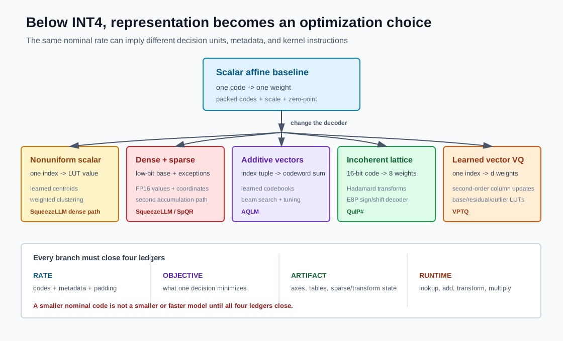
This article owns the following mechanisms:
| Owned here | Deferred owner |
|---|---|
| nonuniform scalar codebooks and sensitivity-weighted clustering | M8.5 |
| dense-and-sparse weight decomposition and high-precision exceptions | M8.5 |
| SpQR’s small groups, hierarchical qparams, and sparse outlier stream | M8.5 |
| additive/multi-codebook quantization and AQLM optimization | M8.5 |
| QuIP/QuIP# weight-Hessian incoherence, BlockLDLQ, and lattice codes | M8.5 |
| VPTQ channel-independent second-order vector quantization | M8.5 |
| general transform-graph equivalence and activation outlier migration | M8.3 |
| live activation and K/V quantization | M8.6 |
| full QAT, STEs, learned quantizer parameters, and distillation | M8.7 |
| native binary/ternary training, BitNet, and OneBit | M8.8 |
| representation serialization, loader support, and decoder kernels | M8.9 |
| production benchmark matrix, release, and rollback | M8.10 |
SqueezeLLM and SpQR are covered by the local A36 source in substantial detail. AQLM, QuIP#, and VPTQ are only lightly represented in the original local corpus, so their mechanisms below are checked directly against their primary papers and official implementations. Published quality and speed numbers are treated as source-reported observations, never as deployment guarantees.
0x01 A Compressed Weight Is A Decoder, Not A Bit Width
Keep the row-major linear convention from M8.1-M8.4:
An extreme-compression artifact does not generally store a low-bit tensor that can be interpreted without context. It stores discrete state , continuous or structured metadata , and a decoder:
The approximation consumed by the model is:
For scalar affine quantization, is one integer per weight and contains scales and zero-points. For a vector codebook, one index may reconstruct weights. For additive quantization, several indices reconstruct one vector by summing codewords. For a dense-and-sparse representation, the decoder adds a sparse correction to a dense low-bit matrix.
The artifact must therefore be described by at least five contracts:
rate contract:
    total bytes, effective bits per original weight, padding, metadata

decoder contract:
    exact function mapping codes and metadata to W_hat

axis contract:
    which weight dimensions are grouped into one scalar/vector decision

optimization contract:
    objective and state used to choose codes, codebooks, or exceptions

runtime contract:
    lookup, unpack, sparse add, transform, and multiply implementation
0x01A Effective Bits Include Everything The Loader Needs
Let be the number of original scalar weights. Define:
The numerator includes every served byte:
Nominal code rate and effective bit rate are equal only when all other terms vanish asymptotically. That assumption is especially dangerous below four bits. A 0.25-bit metadata term consumes one eighth of a two-bit budget.
0x01B Scalar And Vector Rates Count Different Decisions
An ordinary -bit scalar quantizer stores code decisions:
A vector quantizer partitions the same tensor into complete vectors and assigns one of centroids to each vector. For fixed-width random-access codes:
Its fixed-width index rate per scalar is:
log2(K_c) is the information bound for an equiprobable alphabet, not the
physical width of an arbitrary index. With K_c=3,d=2,P=16, fixed-width codes
need 16 bits, not approximately 12.68 bits. Entropy coding has a different,
distribution-dependent rate and random-access contract. Physical packing still
adds byte/word alignment and per-axis vector tails; do not merge row tails merely
to make P/d integral. Power-of-two examples below are unchanged.
But the codebook itself costs:
where is the stored precision of one codebook coordinate. Increasing gives the representation more geometric freedom at a fixed scalar rate, while increasing grows search and codebook storage exponentially. The best reconstruction is not automatically the best kernel.
0x01C Rate, Distortion, And Runtime Form Three Separate Axes
Every method in this article chooses a different compromise:
| Representation | Additional freedom | Additional cost |
|---|---|---|
| nonuniform scalar LUT | learned scalar locations | LUT storage and random lookup |
| dense + sparse | high precision for selected weights | sparse indices, load imbalance, second path |
| additive codebooks | combinatorial sums of codewords | multiple lookups and difficult discrete search |
| transformed lattice VQ | structured high-dimensional packing | transforms and block decoder |
| learned VQ | arbitrary vector centroids | codebook storage, centroid search, cache pressure |
The rest of the article derives those trade-offs rather than ranking method names in isolation.
0x01D NF4: A Distribution-Matched Codebook Is Still Block-Conditioned
NF4, introduced with QLoRA, is an important bridge between ordinary scalar quantization and the learned codebooks below. It stores one four-bit index per scalar, but its 16 reconstruction values are nonuniform. The codepoints are chosen from equal-probability regions under a zero-mean normal model, then normalized into a bounded scalar alphabet that includes an exact zero.
For a block , define the absmax scale:
With fixed NF4 codebook , encode and decode as:
Renderer-safe representation:
block scale: a_B = max_i abs(w_i)
nonzero block: u_i = w_i / a_B
all-zero block: skip division, emit the codebook's exact-zero index
stored scalar: 4-bit index q_i
decoder: w_hat_i = a_B * NF4_CODEBOOK[q_i]
The zero branch is part of the decoder contract, not a magic epsilon. Unlike an
affine scale used as a divisor, this absmax decoder can store a_B=0: zero codes
then reconstruct exactly zero without ever forming 0/0. A backend requiring a
positive sentinel may instead store a declared positive value with the same
exact-zero index; its encoder and decoder must agree. Nonzero scales must remain
positive and finite after their declared storage rounding.
def nf4_block_reference(weights, codebook, round_scale_to_storage):
    if weights.ndim != 1 or weights.size == 0 or not isfinite(weights).all():
        raise ValueError("nonempty finite block required")
    if codebook.ndim != 1 or len(codebook) != 16 or not isfinite(codebook).all():
        raise ValueError("finite sixteen-entry NF4 codebook required")
    zero_indices = nonzero(codebook == 0)[0]
    if len(zero_indices) != 1:
        raise ValueError("one exact-zero reconstruction entry required")
    absmax = float(abs(weights).max())
    if absmax == 0:
        return full(weights.shape, int(zero_indices[0]), dtype=int64), 0.0
    scale = round_scale_to_storage(absmax)
    if not isfinite(scale) or scale <= 0:
        raise ValueError("unrepresentable nonzero block scale")
    normalized = weights / scale
    codes = nearest_index(normalized[:, None], codebook[None, :])
    return codes, scale
This reference takes an explicitly ordered codebook and resolves nearest-distance ties to its lowest index. It illustrates a declared local contract, not every NF4 kernel’s threshold or tie ABI; production parity requires the chosen decoder.
The effective rate already depends on block size and scale representation:
QLoRA’s double quantization compresses the quantization constants themselves, further changing the metadata term. As M6.4 explains, QLoRA optimizes floating adapter factors over a frozen quantized base. That training choice neither fixes the later inference format nor turns frozen codes into QAT parameters; this section owns only the stored scalar representation and geometry.
An important critique from NF4 Isn’t Information Theoretically Optimal (and that’s Good) is narrower than “NF4 is wrong.” Absmax normalization conditions every on the block maximum. The distribution of is therefore not the original unconditioned Gaussian, and it changes with . A fixed codebook derived from the unconditioned model cannot be information-theoretically optimal for every block size. AF4 instead searches for low expected L1 reconstruction error under the block-conditioned distribution while fixing -1, 0, and +1; it is not a global reconstruction-error optimum.
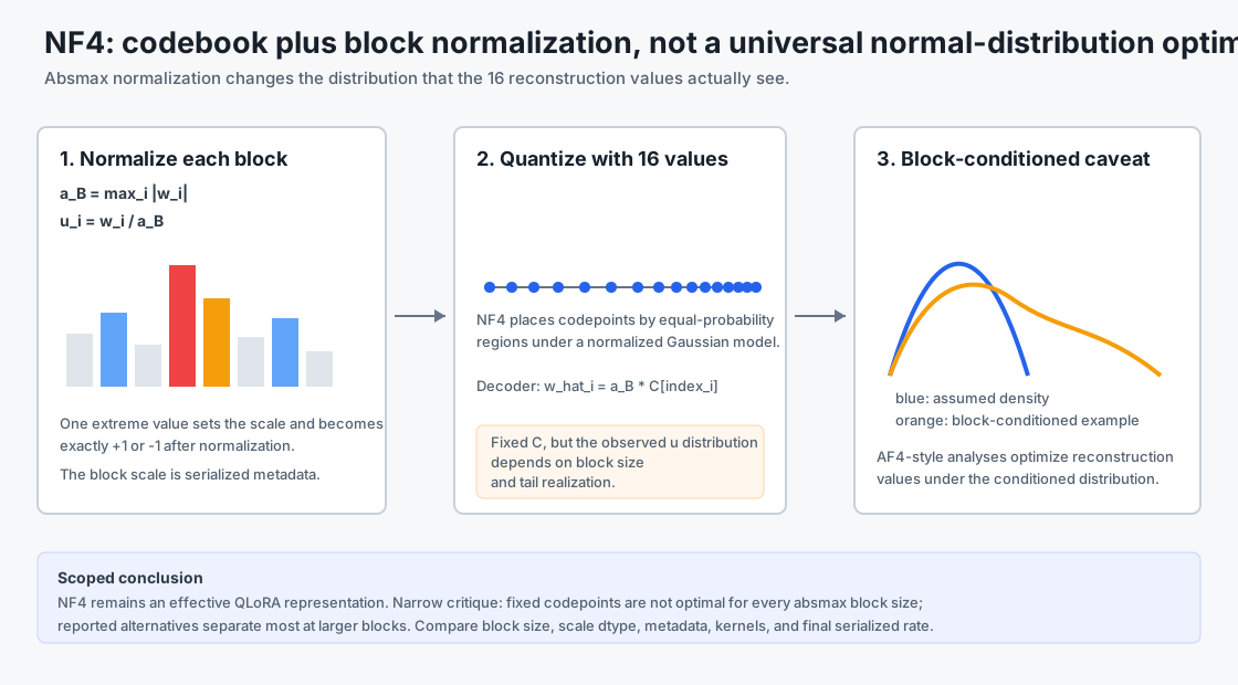
This caveat must remain scoped. The critique reports small empirical differences at common/smaller blocks and larger separation at larger blocks in its studied setup. A representation decision therefore compares:
NF4 versus affine INT4 versus alternative nonuniform codebooks
block size and scale/second-level scale dtype
actual serialized bytes
dequantization/kernel support
held-out task quality, not codebook theory alone
The key conceptual handoff is that a “distribution-matched four-bit type” is actually a tuple of codebook, block normalization, metadata, and decoder. M8.5 will now generalize that tuple to sensitivity-weighted scalar alphabets, sparse exceptions, additive codes, lattices, and learned vector codes.
0x02 Sensitivity-Weighted Nonuniform Scalar Codebooks
Uniform scalar quantization fixes equally spaced reconstruction values. A nonuniform codebook instead stores floating-point centroids:
and reconstructs each scalar weight through an index :
This remains scalar quantization because each decision reconstructs one scalar. What changes is the geometry of the scalar alphabet: adjacent indices need not represent equally spaced values.
0x02A Why Sensitivity Becomes A Clustering Weight
Let collect weights and let be the quantization perturbation. A second-order expansion of a converged model loss is:
If the first-order term is small and the full Hessian is approximated by a diagonal sensitivity matrix,
then:
Substituting the codebook decoder gives:
This is weighted one-dimensional k-means. SqueezeLLM approximates the sensitivity with diagonal Fisher information computed from squared gradients on a calibration set. The approximation is explicit: cross-weight interactions are discarded so a tractable scalar clustering problem remains.
Renderer-safe objective:
J(C, a) = sum_i h_i * (w_i - C[a_i])^2

h_i:
    diagonal Fisher / sensitivity weight

C[a_i]:
    selected nonuniform scalar reconstruction value
0x02B Deriving The Weighted Lloyd Updates
For fixed centroids, one point chooses:
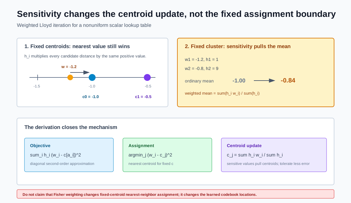
For , the same positive value multiplies every candidate distance for that point, so:
Sensitivity does not change the nearest-centroid assignment boundary when centroids are fixed. It changes where the centroids move.
For a fixed cluster :
Differentiate and set the result to zero:
so:
This quotient requires positive cluster sensitivity mass. If its mass is zero, the objective is independent of that centroid; retain its previous finite value, or re-seed it by one declared deterministic rule, the usual empty-cluster repair. Either choice leaves the weighted objective under the current assignment unchanged, and the next nearest-centroid assignment cannot increase it. Zero-sensitivity points may use deterministic nearest-centroid assignment because every assignment has zero weighted cost. The all-zero-sensitivity case is a defined tie, not a division by zero. For positive mass, the centroid is pulled toward high-sensitivity weights.
0x02C Worked Centroid Trace
Suppose a cluster contains:
| Weight | Sensitivity |
|---|---|
Ordinary k-means places the centroid at:
Sensitivity-weighted k-means places it at:
The high-sensitivity value is reconstructed with error instead of . The low-sensitivity value accepts more error. The method has not made error disappear; it has allocated distortion according to a local loss proxy.
0x02D Code-Level Clustering Contract
def weighted_scalar_codebook(weights, sensitivity, num_codes, iters):
    # weights, sensitivity: [P]
    if weights.ndim != 1 or weights.size == 0 or weights.shape != sensitivity.shape:
        raise ValueError("matching nonempty vectors required")
    if not isfinite(weights).all() or not isfinite(sensitivity).all():
        raise ValueError("nonfinite fitting input")
    if (sensitivity < 0).any() or num_codes < 1 or iters < 0:
        raise ValueError("invalid sensitivity or fitting configuration")
    # Deterministic finite initialization and lowest-index distance ties.
    centroids = initialize_1d_centroids(weights, num_codes)

    for _ in range(iters):
        # Positive h_i cancels; h_i=0 uses the same deterministic tie policy.
        codes = nearest_index(weights[:, None], centroids[None, :])

        for j in range(num_codes):
            members = (codes == j)
            h = sensitivity[members]
            w = weights[members]
            mass = h.sum()
            if not isfinite(mass):
                raise ValueError("sensitivity mass overflow")
            if mass == 0:  # Includes empty and nonempty zero-mass clusters.
                # Default: keep the previous finite centroid. A declared
                # alternative re-seeds it deterministically instead:
                #     centroids[j] = reinitialize_empty_cluster(weights)
                continue
            updated = (h * w).sum() / mass
            if not isfinite(updated):
                raise ValueError("centroid arithmetic overflow")
            centroids[j] = updated

    # Assign against the final codebook, including when iters=0.
    codes = nearest_index(weights[:, None], centroids[None, :])
    return codes, centroids
Implementation invariants:
sensitivity >= 0
every code index < num_codes
empty and zero-mass clusters follow one declared policy:
    retain the previous finite centroid, or re-seed it to a finite value
codebook order is canonicalized before packing
the runtime LUT uses the same code-to-centroid permutation
calibration gradients are excluded from the serving artifact
This explicit zero-mass policy belongs to the generic reference above. The pinned SqueezeLLM fitter instead substitutes uniform sample weights when a whole row’s sample-weight sum is zero before calling its clustering library. Do not silently call those two fallback objectives identical.
0x02E The LUT Is Part Of The Runtime ABI
If each output row of owns a -entry FP16 codebook, then:
For and :
before alignment and headers. This FP16 table is a storage illustration, not a promise about every SqueezeLLM implementation. The kernel performs indexed lookup rather than affine dequantization. The SqueezeLLM paper (Section 4.3) reports 3/4-bit LUT-based matrix-vector kernels that load compressed indices, recover FP16 values piecewise, and perform all arithmetic in FP16 after dequantization; that description is source-reported. Whether the paper’s kernels keep FP16 arithmetic throughout is not externally verified. By contrast, the pinned SqueezeLLM wrapper allocates FP32 lookup tables and sparse-value buffers; its forward path casts inputs to FP32 before its custom 3/4-bit kernels. That Python boundary alone does not establish every CUDA intermediate or accumulator dtype. Record actual stored buffers, operand conversions and kernel arithmetic separately instead of inferring them from the payload bit rate or this FP16 example. A runtime that only accepts affine INT4 cannot consume the LUT artifact without conversion.
0x03 SqueezeLLM: Dense Codes Plus Sparse Exceptions
Nonuniform centroids still face a range problem: a tiny number of extreme weights can pull the codebook away from the dense body of the distribution. SqueezeLLM therefore combines two representation changes:
- sensitivity-weighted nonuniform scalar quantization for the dense component;
- a sparse high-precision component for magnitude outliers and selected sensitive weights, with its actual stored dtype declared.
0x03A The Decomposition And Its Exact Runtime Equation
Write:
where is nonzero only at selected exception coordinates. The served approximation is:
The linear operation becomes:
Some implementations store a full exception value and clear the corresponding dense location. Others store a correction relative to the dense reconstruction. The decoder contract must say which convention is used:
replacement convention:
    W_hat[i,j] = S[i,j] at exception positions

correction convention:
    W_hat[i,j] = Q(D)[i,j] + S[i,j]
The algebra and packer must agree. Adding a full replacement on top of a nonzero dense reconstruction double-counts the weight.
0x03B Outlier Selection And Sensitive-Weight Selection Are Different
Magnitude outliers are selected because they enlarge the representable range. Removing them contracts the range used by dense centroids.
Sensitive weights are selected because a local loss proxy predicts that their quantization error is expensive even when their magnitude is ordinary.
SqueezeLLM uses both:
magnitude path:
    percentile thresholds -> extreme values -> sparse high-precision values

sensitivity path:
    diagonal Fisher estimate -> top sensitive values -> sparse high-precision values

dense path:
    weighted nonuniform k-means on the remaining weights
Conflating the two criteria loses the method’s main design choice. A large weight need not be sensitive, and a sensitive weight need not be large.
0x03C Deriving The Sparse Break-Even Rate
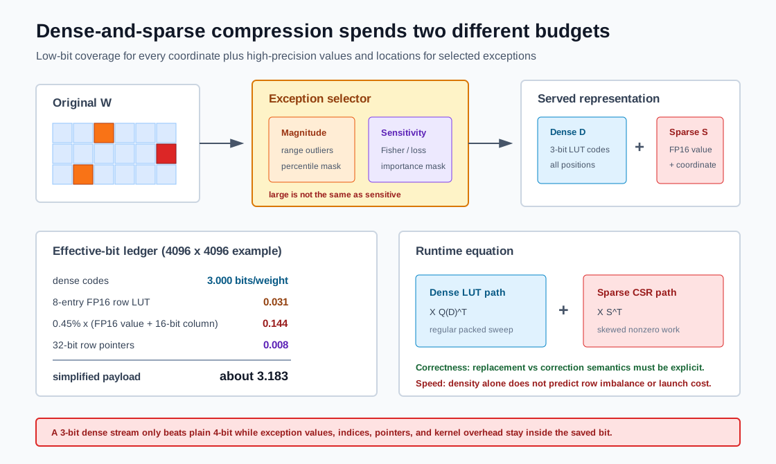
Let be the fraction of exception positions. Suppose the dense stream keeps one -bit code per original position and each sparse exception stores a 16-bit value plus a 16-bit column coordinate. Ignoring lower-order alignment:
For row-wise CSR over an matrix with 32-bit row pointers:
For a 4096-by-4096 matrix, 3-bit row-wise LUTs, and :
Thus the simplified payload is:
The 16-bit widths are an illustration. The pinned SqueezeLLM wrapper described in Section 0x02E stores FP32 lookup tables and sparse values with int32 column indices and row pointers; the same simplified ledger with those widths gives bits per weight, before its optional extra buffers, headers and padding.
This ledger explains both the appeal and the limit. Relative to a plain 4-bit stream, a 3-bit dense stream can spend at most roughly one extra bit per weight on exceptions and metadata. With 32 bits per exception, the rough break-even is below sparsity even before LUTs, pointers, padding, and kernel inefficiency:
Sparse protection is not free precision. It borrows budget from the dense stream.
0x03D Conversion Trace
def squeeze_layer(W, calibration_observations, bits, outlier_pct, sensitive_pct):
    fisher_diag = zeros_like(W, dtype=float32)
    observation_count = 0

    for observation in calibration_observations:
        # One declared observation (e.g. one sequence), not a batch mean.
        loss = model_loss(observation)
        grad_W = grad(loss, W)
        fisher_diag += grad_W.square()
        observation_count += 1
    if observation_count == 0:
        raise ValueError("no sensitivity observations")
    fisher_diag /= observation_count

    magnitude_mask = percentile_outlier_mask(W, outlier_pct)
    sensitivity_mask = top_fraction_mask(fisher_diag, sensitive_pct)
    exception_mask = magnitude_mask | sensitivity_mask

    # Correction convention: dense reconstruction plus sparse correction.
    dense_source = W.masked_fill(exception_mask, 0.0)
    codes, lut = weighted_scalar_codebook_rowwise(
        dense_source,
        fisher_diag,
        valid_mask=~exception_mask,
        num_codes=2 ** bits,
        iters=NUM_LLOYD_ITERS,
    )
    dense = pack_rowwise_codes(codes, lut, exception_mask)

    dense_reconstruction = decode_dense(dense)
    sparse_correction = csr_from_mask(
        W - dense_reconstruction,
        exception_mask,
        value_dtype=float16,
    )

    return DenseSparseArtifact(dense, sparse_correction,
                               sparse_semantics="correction")
The pseudocode emphasizes a representation invariant rather than reproducing one
repository layout. Record the Fisher observation unit, loss/token-mask reduction
and normalization. Squaring a batch-mean gradient is not averaging squared
per-observation gradients: gradients +1,-1 give respectively 0 and 1.
Batched implementations need per-observation gradients (or must explicitly name
the different batch-gradient proxy). Tensor ownership, embedding/output heads,
codebook grouping and serialized exception masks also remain converter contracts.
0x03E Runtime Integration
SqueezeLLM’s paper uses a LUT-based dense kernel and a balanced sparse matrix-vector kernel. The nonzero count is skewed across rows, so assigning one thread per row creates load imbalance. Its balanced sparse strategy assigns similar nonzero work per thread and accepts synchronization where several threads contribute to a row. Dense and sparse work are launched together to reduce the cost of combining outputs.
The deployment lesson is broader than one kernel:
the sparse rate must be measured after indices and row pointers
the nonzero distribution must be profiled, not only its mean
the dense and sparse outputs must share accumulation semantics
the two paths must not serialize into two bandwidth sweeps unnecessarily
prefill and decode need separate measurements
0x04 SpQR: Sensitivity, Tiny Groups, And Hierarchical Metadata
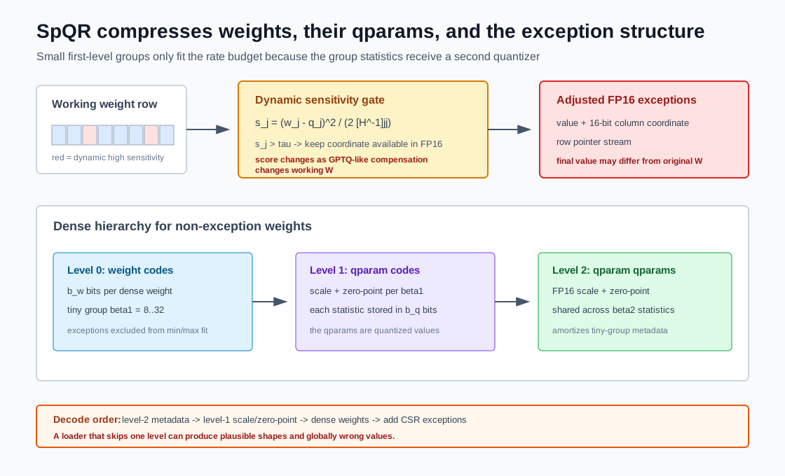
SpQR also protects a sparse set of high-precision weights, but it is not SqueezeLLM with a different threshold. Its dense representation remains a small-group scalar quantizer, and it attacks metadata overhead by quantizing the quantization parameters themselves.
0x04A Deriving The Dynamic Sensitivity Test
For one output row, let the local reconstruction objective be:
where is induced by calibration activations as in M8.4. Force weight coordinate to move by:
while allowing all other coordinates to compensate optimally. The OBS/OBQ constrained solution gives the minimum loss increase:
This score is large when the scalar rounding error is large, when the coordinate is hard to compensate through correlated directions, or both. SpQR can evaluate the criterion dynamically while processing columns with GPTQ-like state, so the score reflects compensation already applied by earlier decisions.
The exception criterion can be expressed as:
For a protected FP16 weight, the direct quantization error term is removed. The threshold is chosen to reach a target global exception budget rather than a fixed magnitude percentile.
0x04B Why Very Small Groups Need A Second Quantizer
Let first-level groups contain consecutive weights. Every group stores its own scale and zero-point. Smaller fits local range changes better, but raw FP16 qparams cost:
At , raw scale and zero-point metadata alone cost two bits per weight. That would erase much of a 3-bit compression target.
SpQR groups first-level statistics and quantizes those statistics to bits. A simplified two-stream ledger is:
The terms are:
b_w:
    dense low-bit weight code

2*b_q / beta_1:
    quantized first-level scale and zero-point

64 / (beta_1*beta_2):
    simplified FP16 scale/zero-point metadata for two
    second-level qparam streams

32*rho + row pointers:
    FP16 outlier value and 16-bit column coordinate in CSR
Exact layouts may interleave, share, or pad qparam streams differently. The formula is a design ledger, not a claim that every SpQR implementation uses this byte-for-byte ABI.
With , , and :
The result explains how tiny groups and FP16 exceptions can still approach a four-bit effective rate: qparams are themselves compressed.
0x04C The Exception May Be An Optimized Weight, Not The Original Weight
SpQR excludes detected outliers when fitting each dense group’s quantization statistics, quantizes the remaining base weights, and uses GPTQ-like compensation. A high-precision exception can absorb error from other weights. Therefore, its final FP16 value need not equal the original pretrained scalar at that coordinate.
This distinction matters:
outlier preservation:
    store original W[i,j] because it is large or sensitive

optimized exception:
    store a high-precision value at (i,j) that may have moved
    to compensate dense quantization error elsewhere
Calling every exception an “original outlier” hides the solver’s role.
0x04D Conversion And Packing Trace
def spqr_row(row, H_inv, beta1, beta2, weight_bits, qparam_bits, tau):
    working = row.clone()
    exception_entries = []
    dense_groups = []
    first_level_qparams = []

    for group_cols in consecutive_groups(len(row), beta1):
        candidate = working[group_cols]
        provisional_grid = fit_affine_grid(candidate, weight_bits)

        errors = provisional_grid.quantize(candidate) - candidate
        sensitivity = errors.square() / (2 * diag(H_inv)[group_cols])
        is_exception = sensitivity > tau

        base_values = candidate[~is_exception]
        qparams = fit_affine_grid(base_values, weight_bits)
        codes = quantize(base_values, qparams)

        dense_groups.append(pack_codes_with_holes(codes, is_exception))
        first_level_qparams.append(qparams)

        # GPTQ-style update changes still-unquantized state. Exception
        # coordinates remain available to absorb compensation.
        working = compensate_trailing_columns(
            working, group_cols, codes, qparams, H_inv, is_exception
        )

        exception_entries.extend(
            collect_adjusted_fp16_exceptions(working, group_cols, is_exception)
        )

    qparam_codes, second_level_qparams = quantize_qparams(
        first_level_qparams, group_size=beta2, bits=qparam_bits
    )

    return pack_spqr_row(
        dense_groups,
        qparam_codes,
        second_level_qparams,
        exception_entries,
    )
The actual algorithm interleaves outlier detection, group quantization, qparam compression, and compensation more carefully than this teaching sketch. The important trace is that holes, dense code positions, qparam indices, and adjusted sparse coordinates all share one original tensor coordinate system.
0x04E SqueezeLLM And SpQR Make Different Design Choices
| Dimension | SqueezeLLM | SpQR |
|---|---|---|
| dense scalar alphabet | learned nonuniform LUT | grouped affine low-bit grid |
| sensitivity proxy | diagonal Fisher weighting and sparse selection | OBS/OBQ-style dynamic quantization sensitivity |
| range handling | magnitude outliers in sparse component | outliers excluded from tiny-group qparams |
| qparam strategy | row/channel LUT entries | tiny first-level groups plus quantized qparams |
| exception semantics | outliers and sensitive values; stored dtype is implementation-specific | high-sensitivity adjusted FP16 exceptions |
| runtime | LUT dense GEMV + balanced sparse GEMV | dense dequantization + CSR exception path |
Both papers report favorable compression/quality/runtime results in their evaluated settings. Those numbers do not establish that either compound sparse format is faster than a dense scalar kernel on another GPU, batch shape, or implementation.
0x05 AQLM: Additive Quantization Changes One Code Into A Tuple
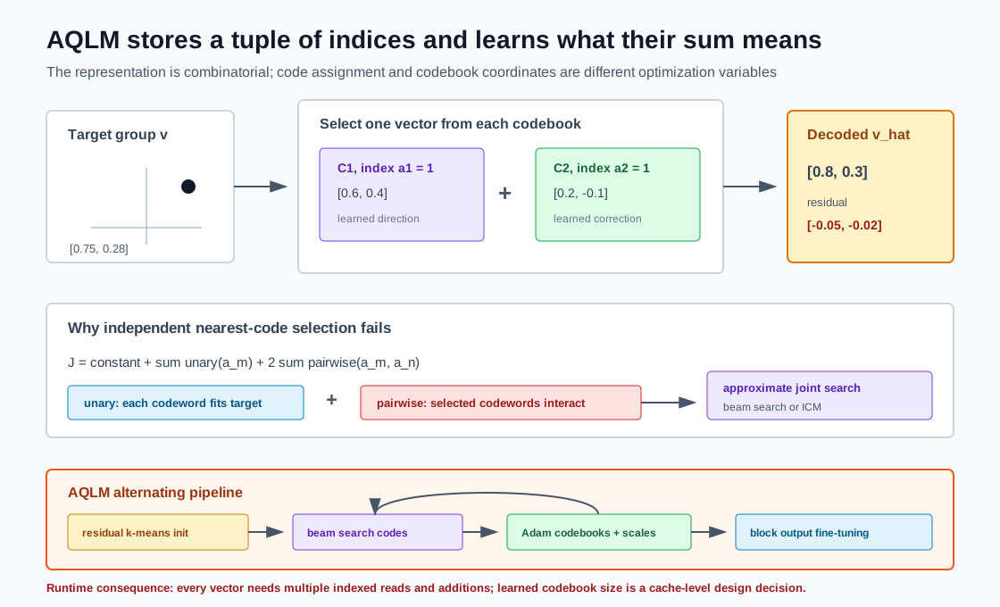
Sparse exceptions preserve selected scalars. Additive quantization changes the dense representation itself. It partitions weight rows into -dimensional groups and reconstructs each group as a sum of codewords from codebooks.
Let codebook contain vectors:
For weight vector , store indices and decode:
where is commonly an output-row scale.
The representable set contains as many as sums, although codeword interactions mean those sums need not be unique or uniformly distributed.
0x05A Product, Residual, And Additive Quantization Are Not Synonyms
| Family | Reconstruction | Constraint |
|---|---|---|
| product quantization (PQ) | concatenate subvector codewords | each codebook owns disjoint dimensions |
| residual vector quantization (RVQ) | later codebooks are trained on prior residuals | |
| additive quantization (AQ) | codebooks jointly span the full vector; no residual-order constraint |
RVQ is an initialization or constrained model of the residual sequence. General AQ can revise all codebooks jointly after initialization and usually has a harder discrete assignment problem.
0x05B Rate Derivation
There are complete weight vectors. Each of fixed-width indices uses
bits; log2(K_c) alone is only the equiprobable
information bound. Add per-axis tails and actual packing separately:
The nominal scalar rate is:
The learned codebooks cost:
If one codebook set is stored per matrix and one FP16 scale per output row:
At small matrices or large learned codebooks, codebook bytes are not negligible. AQLM configurations using one FP16 codebook have a 16-bit vector index, hence two nominal bits per scalar, but the codebook alone occupies roughly one MiB per linear layer. That quality-oriented representation can pressure cache and runtime even though its index rate is only two bits.
0x05C The PTQ Objective Is Input-Adaptive Additive Quantization
For a linear layer, AQLM minimizes output reconstruction on calibration inputs:
Let . Then:
Define the input Gram matrix:
Then:
This is why AQLM is not ordinary k-means on weight vectors. Calibration activations define which reconstruction directions matter.
0x05D Why Code Assignment Becomes A Coupled Discrete Problem
Consider one embedded weight group with target and additive reconstruction:
Using a local Gram block , its error is:
Expand:
The first term is constant. The next two produce per-code unary costs. The final sum produces pairwise interactions between codebook choices. Selecting the nearest codeword from each codebook independently is therefore not generally optimal.
The code tuple can be viewed as a fully connected discrete Markov random field:
unary potential:
    how one selected codeword fits the target under G

pairwise potential:
    how two selected codewords interact under G

exact joint search:
    exponential in the number of codebooks

AQLM approximation:
    beam search over code replacements, parallel over output rows
This derivation explains why additive representation quality comes with conversion cost.
0x05E AQLM’s Three Optimization Phases
Phase 0: residual k-means initialization
The first codebook clusters weight groups. Its selected codewords are subtracted. The second codebook clusters the residual, and so on. This gives every later codebook a useful starting role before joint optimization.
Phase 1: discrete code update
With codebooks fixed, AQLM uses beam search. It starts from the current code tuple, tries alternatives for one code, retains the best candidate tuples, and updates incremental MSE terms rather than recomputing the entire objective. Randomized iterative conditional modes is an alternative; the paper chose beam search partly because it maps conveniently to PyTorch/JAX execution.
Phase 2: continuous codebook and scale update
With discrete codes fixed, the problem is continuous. In principle it is a least-squares problem, but activation weighting couples codebook coordinates. AQLM’s implementation uses full-batch Adam steps to optimize codebooks and per-output scales, then alternates back to discrete search until improvement falls below a tolerance.
Phase 3: transformer-block fine-tuning
Independent linear-layer reconstruction misses error interactions through attention, residual paths, normalization, and the MLP. After quantizing the linear layers of one transformer block, AQLM minimizes block-output MSE:
The discrete codes stay frozen. The trainable state includes codebook coordinates, row scales, and small non-quantized parameters such as RMSNorm scales/biases. This is post-training refinement, not low-bit pretraining. Full QAT remains M8.7’s owner.
0x05F End-To-End Conversion Trace
def aqlm_convert(model, calibration):
    block_input = model.embed(calibration.tokens)

    for block in model.blocks:
        reference_output = block.fp_forward(block_input).detach()

        for linear in block.linear_layers():
            X = capture_linear_inputs(linear, block_input)
            G = X.T @ X

            codebooks, codes, scales = residual_kmeans_init(
                linear.weight,
                vector_dim=VECTOR_DIM,
                num_codebooks=NUM_CODEBOOKS,
                entries=CODEBOOK_SIZE,
            )

            while improvement_above_tolerance():
                codes = beam_search_codes(
                    linear.weight, G, codebooks, codes, scales
                )
                codebooks, scales = optimize_continuous_state_adam(
                    linear.weight, G, codebooks, codes, scales
                )

            linear.replace_with_aqlm(codebooks, codes, scales)

        # Codes remain discrete and frozen. Codebooks, scales, and small
        # unquantized parameters recover interactions within the block.
        trainable = block.codebooks_and_scales_and_norms()
        adam_minimize(
            mse(block(block_input), reference_output),
            parameters=trainable,
        )

        block_input = block(block_input).detach()

    return model
0x05G A Two-Dimensional Additive Trace
Let two one-bit codebooks be:
For target:
choose the second entry from both codebooks:
The residual is:
Two one-bit indices encode the two-dimensional vector, or one nominal bit per scalar before codebook overhead. The useful point is not that this toy always beats a scalar quantizer. It shows that representable vectors are sums of learned directions rather than a Cartesian product of one scalar alphabet.
0x05H Runtime Choices
An additive decoder can be integrated in several ways:
materialize then GEMM:
    unpack indices -> sum codewords -> write W_hat -> regular GEMM
    simple, but rereads/writes a large temporary tensor

fused decode-multiply:
    lookup codewords in registers/shared cache -> multiply activation tile
    avoids W_hat in HBM, but kernel is representation-specific

lookup inner products:
    precompute activation dot codeword, then sum indexed results
    can reduce arithmetic for some shapes, but changes tiling/cache behavior
Learned unstructured codebooks may improve reconstruction while producing random lookup traffic and large cache footprints. That is the central AQLM-versus-QuIP# design contrast, not an incidental implementation detail.
0x06 QuIP And QuIP#: Incoherence Before Lattice Coding
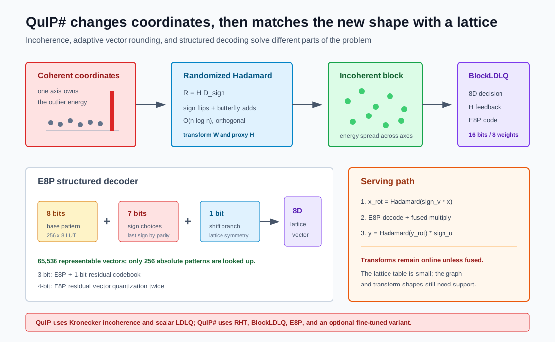
QuIP starts from a different diagnosis. Extreme quantization is difficult when weights contain coordinate spikes and when the important eigenvectors of the proxy Hessian align strongly with coordinate axes. Instead of storing those coordinates as exceptions, QuIP applies random orthogonal transforms that spread both weight energy and curvature directions before rounding.
QuIP# then pairs the transformed distribution with block adaptive rounding and a structured eight-dimensional lattice codebook.
0x06A The Incoherence Condition
For , weight incoherence bounds individual coordinates relative to total Frobenius energy:
For Hessian eigendecomposition , Hessian incoherence bounds eigenvector coordinates:
Informally:
weight incoherence:
    no scalar coordinate owns too much weight energy

Hessian incoherence:
    no coordinate axis aligns too strongly with an important curvature direction
This is stronger and more precise than saying that a rotation “makes values Gaussian.”
0x06B Deriving Objective Preservation Under Two-Sided Rotation
Let and be orthogonal:
Transform weights and curvature:
Let and . The proxy loss in transformed coordinates is:
Substitute:
Use :
By cyclicity of trace and :
The orthogonal change of basis preserves the unquantized quadratic objective. Quantization is basis-dependent, so the transformed coordinates can be easier to approximate even though the floating-point problem is equivalent.
The runtime identity follows from:
For a row activation :
The input is transformed by , the compressed is decoded/multiplied, and the output is transformed by . Some transforms can be fused into adjacent graph edges; otherwise they are online work.
0x06C QuIP Versus QuIP# Incoherence Processing
| Method | Structured orthogonal transform | Main implication |
|---|---|---|
| QuIP | Kronecker products of smaller random orthogonal factors | principled weight/Hessian incoherence with structured runtime |
| QuIP# | randomized Hadamard transform (RHT) | stronger concentration bound and fast transform |
For normalized Hadamard and random sign diagonal :
Multiplication by flips signs. The fast Walsh-Hadamard transform then performs butterfly additions/subtractions. For power-of-two dimensions, the cost is and requires no general floating-point matrix multiply.
QuIP# also describes factored Hadamard constructions and a randomized FFT fallback for dimensions that do not admit a convenient Hadamard factorization. The transform shape and sign vectors are therefore part of the artifact manifest.
0x06D From LDLQ To BlockLDLQ
Scalar LDLQ rounds columns with feedback from previous rounding error. If:
is an LDL factorization, its feedback matrix is derived from . In scalar form:
Vector quantization rounds a block of columns together. QuIP# replaces the scalar factorization with a block LDL decomposition and uses block feedback:
contains the feedback columns for the current block. The vector quantizer maps each -dimensional row block to a codeword. BlockLDLQ therefore preserves the second-order compensation idea while changing the atomic rounding decision from a scalar to a vector.
0x06E Why The E8P Codebook Is Structured
A generic -bit-per-coordinate VQ over dimensions contains:
vectors. At two bits per coordinate and , that is:
eight-dimensional codewords. An unstructured FP16 table would be too large for the intended fast lookup path.
QuIP# constructs E8P from the highly symmetric lattice. Its 16-bit vector code is decoded as:
8 bits:
    select one of 256 stored absolute base patterns

7 bits:
    explicit sign choices

1 bit:
    select the lattice shift / parity branch

implicit final sign:
    recovered from parity
Thus the full representable set only needs lookup into a base table plus inexpensive sign/shift operations. The paper reports a 1 KiB base codebook, small enough for the intended GPU cache path.
The nominal rate remains:
But unlike an arbitrary learned 65,536-by-8 table, its decoder exploits lattice symmetry.
0x06F Higher Rates Use Residual Lattice Codes
The full lattice codebook grows exponentially with bitrate. QuIP# uses residual vector quantization instead:
The paper’s design uses two-bit E8P once for two-bit weights, combines it with a one-bit lattice codebook for three bits, and applies E8P twice for four bits. General AQ could optimize codebooks jointly, but QuIP# chooses structured RVQ to preserve a compact and fast decoder.
0x06G Fine-Tuning Is Part Of The QuIP# Variant
QuIP# separates three effects in its ablations:
RHT + scalar/unstructured alternative:
    benefit from incoherence processing

RHT + E8P without fine-tuning:
    additional benefit from lattice shaping

RHT + E8P + fine-tuning:
    recovery of inter-layer error
Within transformer blocks, unquantized layers are tuned to compensate for already quantized layers before their own quantization. After all linear layers are quantized, remaining unquantized parameters are tuned against full-model activation error. The sign vectors may be relaxed from binary signs to FP16 trainable vectors; their matrix-size-amortized storage remains small in the paper’s bit ledger.
This is more state than pure GPTQ conversion and less than native low-bit pretraining. A release manifest must record whether the checkpoint is NoFT, block-tuned, or end-to-end tuned.
0x06H Runtime Trace
For this trace, use normalized symmetric power-of-two Hadamard matrices,
and , with binary sign diagonals and
. For row activations, fast_hadamard(z) means right
multiplication by the dimension-matched . Therefore
, but :
input signs precede the Hadamard and output signs follow it. The order also
matches the pinned QuIP# inverse transform.
Factored/FFT transforms and fine-tuned nonbinary vectors need their own recorded
conventions; this orthogonal identity does not certify those runtime variants.
def quip_sharp_linear(x, artifact):
    # x: [..., K]
    x_rot = fast_hadamard(x * artifact.input_sign)

    # Packed 16-bit codes represent eight weights each. The decoder
    # performs a 256-entry base lookup, sign/parity reconstruction,
    # and fused multiply without materializing the full W_hat in HBM.
    y_rot = e8p_decompress_multiply(
        artifact.packed_codes,
        artifact.e8p_base_table,
        x_rot,
        artifact.stage_scales,
    )

    y = fast_hadamard(y_rot) * artifact.output_sign
    return y
The QuIP# paper reports proof-of-concept kernels and source-specific throughput. The reusable engineering claim is narrower: a structured codebook that fits in cache can produce a more regular decoder than a large learned table. Actual speed still depends on transform fusion, model dimensions, batch shape, GPU, and software version.
0x07 VPTQ: Second-Order Vector Decisions One Column At A Time
VPTQ uses learned vector centroids, but its tensor orientation and optimization differ from AQLM.
AQLM vector group:
    consecutive input dimensions within one output row
    reconstruction = sum of multiple codewords

VPTQ vector group:
    consecutive output coordinates within one input column
    reconstruction = one centroid, optionally plus residual centroid
This orientation lets VPTQ retain a GPTQ-like column sequence while quantizing chunks of each column with vector lookup.
0x07A Why Vector Quantization Can Beat Scalar Rate Geometry
For vector length and centroids:
The equiprobable information rate is bits per scalar; fixed-width indices use before codebooks, tails and packing.
Use the VPTQ paper’s illustrative matrix:
The FP16 original costs:
The codebook costs:
There are vectors, each with an eight-bit index:
The resulting effective width is approximately bits per scalar before broader artifact overhead. At roughly one bit per scalar, a scalar alphabet has only two values per coordinate; the VQ decoder chooses among 256 learned eight-dimensional shapes.
0x07B Deriving Channel-Independent Second-Order Selection
Use the damped layer proxy with positive-definite :
Suppose input column is the current decision. VPTQ partitions into vectors of length over output coordinates and chooses one centroid for each vector. Let be the inverse curvature of the remaining coordinates after damping; its leading coordinate represents column .
Under the same constrained second-order argument used by OBQ/GPTQ, forcing the column to produces the minimum loss increase:
While selecting centroids for a fixed column, is a positive scalar shared by every vector candidate. Therefore:
Each output vector can use ordinary nearest-centroid lookup after prior columns have updated the working weight state. The Hessian still matters through error propagation:
The current column becomes its selected VQ reconstruction. The direct path must then remove that coordinate by the Schur downdate from M8.4; reusing the raw full inverse does not implement this reduced constrained optimum.
The lazy listing below instead uses the equivalent fixed upper factor with . Its scaled error divides by and its update uses , not the full inverse’s diagonal/row. This typed teaching reference makes the state explicit; it is not a claim to reproduce every detail of the VPTQ paper’s Algorithm 1 or to recover a converter ABI from an inference repository.
0x07C VPTQ Versus GPTVQ Update Granularity
GPTVQ quantizes several input columns jointly as one vector decision. Error from those columns is propagated after the whole vector block is chosen. VPTQ instead makes VQ decisions within one column over output-coordinate chunks, then propagates that column’s error immediately.
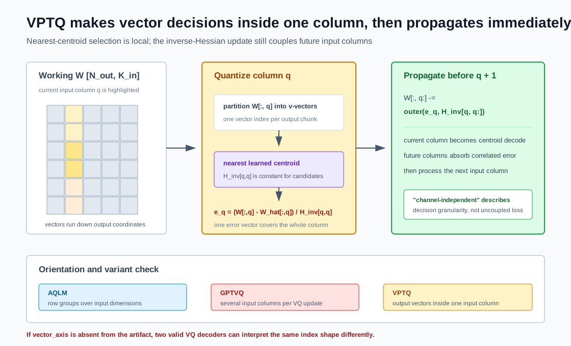
This is the meaning of channel-independent second-order optimization in the paper. It does not mean that columns are independent in the final objective. The Hessian update explicitly couples current error into later columns.
0x07D Hessian-Weighted Centroid Initialization
Before sequential quantization, VPTQ needs a codebook. Expand the proxy loss by columns:
If the diagonal dominates during initialization, keep the first term:
After partitioning each column into vectors, this is weighted vector k-means. Vectors drawn from input column receive weight . The full sequential second-order algorithm then restores off-diagonal compensation that the initialization ignored.
0x07E Residual And Outlier Codebooks
VPTQ extends its base VQ in two ways.
Residual VQ encodes the base error with another codebook:
Outlier quantization identifies columns or tiles with large Hessian-weighted difficulty and gives them a separate codebook. Unlike SqueezeLLM/SpQR, this is not necessarily a high-precision sparse exception stream (16-bit values in both papers; FP32 values in the pinned SqueezeLLM code). It is a specialized VQ alphabet for the difficult subset.
These are alternative places to spend bits:
larger base codebook:
    more entries for every vector

residual codebook:
    second index models remaining error

outlier codebook:
    specialized entries only for difficult columns/tiles

longer vector:
    more correlation per decision, harder centroid fit
0x07F Conversion Trace
def vptq_matrix(W, R, vector_dim, codebook, block_cols):
    # W: [N_out, K_in]; fixed upper R satisfies H_d^-1 = R.T @ R.
    if vector_dim < 1 or W.shape[0] % vector_dim or block_cols < 1:
        raise ValueError("complete output vectors and positive block size required")
    require_upper_positive_factor(R, W.shape[1])
    working = W.clone()
    packed_indices = zeros((W.shape[0] // vector_dim, W.shape[1]), dtype=int64)

    for block_start in range(0, W.shape[1], block_cols):
        block_end = min(block_start + block_cols, W.shape[1])
        scaled_errors = zeros(
            (W.shape[0], block_end - block_start), dtype=working.dtype
        )

        for q in range(block_start, block_end):
            column_vectors = working[:, q].reshape(-1, vector_dim)
            index = nearest_centroid(column_vectors, codebook)
            q_vectors = codebook[index]
            q_column = q_vectors.reshape(-1)

            packed_indices[:, q] = index

            error = (working[:, q] - q_column) / R[q, q]
            scaled_errors[:, q - block_start] = error
            working[:, q:block_end] -= outer(error, R[q, q:block_end])

        # Lazy update outside the block uses the same scaled errors that drove
        # the sequential in-block compensation.
        working[:, block_end:] -= (
            scaled_errors @ R[block_start:block_end, block_end:]
        )

    return packed_indices
A full VPTQ converter also performs Hessian-weighted codebook initialization, optional residual/outlier passes, per-layer parallelization, and optional layer refinement. During layer refinement, the paper updates codebook centroids and small normalization parameters against original-versus-quantized layer output MSE.
0x07G Runtime Decoder
The serving artifact contains an index matrix and one or more codebooks. Runtime reconstructs vector tiles by lookup before or during the linear operator:
def vptq_decode_tile(base_index, base_codebook,
                      residual_index=None, residual_codebook=None,
                      outlier_index=None, outlier_codebook=None):
    tile = base_codebook[base_index]

    if residual_index is not None:
        tile = tile + residual_codebook[residual_index]

    if outlier_index is not None:
        tile = select_outlier_reconstruction(
            tile, outlier_codebook[outlier_index]
        )

    return tile
The VPTQ paper reports lower conversion time and higher throughput than compared methods in its setup. That is source-reported. The architectural claim that survives across systems is that its online path is codebook lookup without QuIP#‘s Hadamard postprocessing, while its learned codebooks and optional residual/outlier streams still create cache, packing, and kernel constraints.
0x08 The Representation Is The Kernel’s Instruction Set
The five families now expose different inner loops:
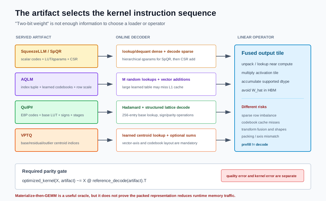
| Method | Served codes | Continuous/structured state | Online decode | Main irregularity |
|---|---|---|---|---|
| scalar affine baseline | one scalar index/weight | scales, zero-points | affine dequantize | group metadata |
| SqueezeLLM | scalar LUT index + sparse coordinates | row/channel LUT + declared high-precision exceptions | LUT dense path + sparse add | unstructured nonzeros |
| SpQR | scalar code + qparam code + sparse coordinates | second-level qparams + FP16 exceptions | hierarchical qparam decode + dense/sparse | tiny groups and CSR |
| AQLM | tuple of indices/vector | learned codebooks + row scales | multiple lookup/add operations | large random-access codebooks |
| QuIP# | structured 16-bit code/8-vector | E8P base table + signs + stage scales | Hadamard, lattice decode, multiply, Hadamard | transform/fusion constraints |
| VPTQ | one or more centroid indices/vector | learned base/residual/outlier codebooks | lookup and optional vector sums | codebook/cache/layout |
| QMoE | UINT16 fixed-to-variable dictionary code | shared ternary-sequence dictionary + row offsets + row reconstruction values | warp dictionary decode fused with expert matrix-vector multiply | variable decoded length and MoE expert residency |
For each row, the selected kernel additionally supplies input, decoded-operand,
scale-application, accumulation and epilogue dtypes, plus overflow bounds/tests.
These are runtime_specific_unknown until supplied by that exact kernel; neither
two-bit payload nor an FP16 codebook proves FP16 or FP32 accumulation. Unknown
fields block production admission, not a source-reported representation overview.
0x08A QMoE: Sub-One-Bit Is A Dictionary Decoder, Not A Fractional Scalar Type
MoE models create an unusual compression opportunity. Only selected experts execute for a token, but all expert weights must be resident or available. QMoE targets that large dormant capacity with retraining-free ternary compression and a custom fixed-to-variable dictionary format co-designed with a GPU matrix-vector kernel.
The paper observes high natural frequency of the zero ternary symbol in its compressed Switch Transformer experts. A naive two-bit ternary stream still costs two bits/weight; a one-bit sparsity mask already spends the desired budget before values and indices. QMoE instead assigns one fixed-width UINT16 codeword to a variable-length sequence of ternary pairs.
Its shared dictionary has entries. One dictionary entry contains up to 14 pairs, or 28 ternary weights, packed into two 32-bit words plus a repeated four-bit pair count. A codeword that expands to weights has payload rate:
before row offsets, row reconstruction values, dictionary storage, alignment, and padding. Sub-one-bit payload therefore requires average expansion . It does not mean that a hardware scalar has width bits.
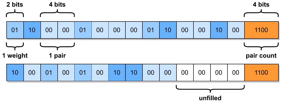
Source: QMoE, Figure 4, arXiv:2310.16795, CC BY 4.0. The illustrated entry represents 24 weights; the format supports up to 28. Labels and bit allocation are source-reported.
The full effective-rate ledger is:
The shared dictionary is deliberately static so it can be reused across many expert matrices and remain cache-resident. The GPU decoder lets one warp process one codeword, uses the pair count to divide useful decoded symbols, and fuses reconstruction with matrix-vector multiplication. That kernel contract influenced the compression format: a more entropy-optimal variable-length bitstream could serialize smaller and still diverge or execute poorly on warps.
def qmoe_reference_decode(codewords, row_offsets, dictionary,
                          row_ternary_values):
    rows = []
    for row in range(len(row_offsets) - 1):
        symbols = []
        for code in codewords[row_offsets[row]:row_offsets[row + 1]]:
            packed_pairs, pair_count = dictionary[code]
            symbols.extend(unpack_ternary_pairs(packed_pairs, pair_count))

        zero, negative, positive = row_ternary_values[row]
        rows.append(map_symbols(symbols, [zero, negative, positive]))
    return stack(rows)
QMoE reports compressing SwitchTransformer-c2048 from a 3.2 TB BF16 representation to under 160 GB, approximately 0.8 bits/parameter, with source-reported quality and runtime results. This is a system-specific artifact rate for a very sparse large-MoE weight distribution, not a general promise for dense decoder LLMs. M6.2 owns semantic routing and load balance; M6.6 owns physical expert placement, collectives, grouped execution and measured runtime. M8.5 owns the dictionary ABI and fused-decoder representation boundary.
0x08B A Generic Artifact Schema
@dataclass
class ExtremeWeightArtifact:
    family: str                 # lut_sparse, spqr, aqlm, e8p, vptq, qmoe_dict
    original_shape: tuple[int, int]
    vector_axis: str | None     # input-row groups or output-column chunks
    vector_dim: int | None

    packed_codes: Tensor
    codebooks: list[Tensor]
    scales: Tensor | None

    sparse_values: Tensor | None
    sparse_col_indices: Tensor | None
    sparse_row_ptr: Tensor | None
    sparse_semantics: str        # correction | replacement | none
    dense_hole_policy: str       # ignored_by_overwrite | zero_mask | none
    duplicate_coordinate_policy: str  # reject
    coordinate_dtype: str
    combine_order: str          # decode_dense_then_add | decode_dense_then_replace

    input_transform: TransformSpec | None
    output_transform: TransformSpec | None

    packing_layout: str
    decoder_version: str
    required_kernel: str
    operator_contract: dict     # input_dtype, decoded_operand_dtype,
                                # scale_application_dtype, accumulator_dtype,
                                # epilogue_dtype, overflow_bound_or_test
This is a conceptual schema, not a proposed universal format. It makes hidden contracts visible:
- AQLM and VPTQ can both say “vector quantization” while grouping opposite tensor axes.
- Two-bit QuIP# means 16 index bits per eight-dimensional vector, not a two-bit scalar code stream.
- A sparse exception artifact needs coordinate width and replacement/correction semantics.
- A codebook checksum matters as much as a scale checksum; changing codebook order corrupts every index.
- A transform-aware artifact must state sign-vector precision and whether transforms are fused into graph neighbors.
0x08C Reference Decoder Before The Optimized Kernel
Every representation should have a slow, explicit decoder used as an oracle:
The two sparse reference profiles below require either explicit overwrite replacement or addition of corrections against the fully decoded dense stream. Other hole/combination policies are rejected until separately implemented; merely zeroing the source weight does not guarantee that its LUT reconstruction is zero.
def combine_dense_sparse(dense, artifact):
    # Validation rejects duplicate/out-of-bounds coordinates, even for zeros.
    rows, cols, values = validated_unique_csr_entries(artifact, dense.shape)
    result = dense.clone()
    if artifact.sparse_semantics == "replacement":
        require(artifact.combine_order == "decode_dense_then_replace")
        require(artifact.dense_hole_policy == "ignored_by_overwrite")
        result[rows, cols] = values
    elif artifact.sparse_semantics == "correction":
        require(artifact.combine_order == "decode_dense_then_add")
        require(artifact.dense_hole_policy == "none")
        result[rows, cols] += values
    else:
        raise ValueError("unsupported sparse decoder contract")
    return result


def reference_weight(artifact):
    if artifact.family == "lut_sparse":
        dense = decode_scalar_lut(artifact.packed_codes, artifact.codebooks)
        return combine_dense_sparse(dense, artifact)

    if artifact.family == "spqr":
        qparams = decode_hierarchical_qparams(artifact)
        dense = decode_grouped_scalar(artifact.packed_codes, qparams)
        return combine_dense_sparse(dense, artifact)

    if artifact.family == "aqlm":
        vectors = sum(
            C[idx] for C, idx in zip(artifact.codebooks, unpack_indices(artifact))
        )
        return apply_row_scales(unvectorize(vectors), artifact.scales)

    if artifact.family == "e8p":
        transformed = decode_e8p(artifact.packed_codes, artifact.codebooks[0])
        return inverse_two_sided_transform(transformed, artifact)

    if artifact.family == "vptq":
        vectors = decode_base_residual_outlier_codebooks(artifact)
        return unvectorize_columns(vectors, artifact.original_shape)

    if artifact.family == "qmoe_dict":
        return qmoe_reference_decode(
            artifact.packed_codes,
            artifact.sparse_row_ptr,
            artifact.codebooks[0],
            artifact.scales,
        )

    raise UnsupportedRepresentation(artifact.family)
Required equivalence test:
Quality evaluation compares the reference decoded model with FP16. Kernel correctness compares the optimized kernel with the reference decoded model. Mixing those two errors makes debugging needlessly ambiguous.
0x09 Calibration, Optimization, And Training State
Calling every method “PTQ” does not mean they have the same conversion cost or state.
| Method | Calibration evidence | Discrete optimization | Continuous optimization | Inter-layer refinement |
|---|---|---|---|---|
| SqueezeLLM | gradient/Fisher samples | nearest LUT assignment + sparse selection | weighted centroids | none in core method |
| SpQR | layer activations / inverse curvature | scalar codes + dynamic exception selection | compensation state, qparams | none in core method |
| AQLM | linear/block inputs and outputs | beam search over code tuples | codebooks + scales with Adam | block tuning; optional end-to-end variant |
| QuIP# | proxy Hessians + development set | BlockLDLQ lattice codes | scale/sign and remaining parameters in FT variant | within-block and end-to-end refinement |
| VPTQ | proxy Hessians + layer outputs | nearest vector codes in sequential update | centroids and norms in optional tuning | optional layer/end-to-end refinement |
| QMoE | expert-token calibration buffers and ternary statistics | ternary assignment + dictionary encoding | row reconstruction values | none in core retraining-free pipeline |
The deployment manifest should record:
calibration dataset identity and valid-token count
captured tensor shapes and orientation
Gram/Hessian accumulation dtype and damping
codebook initialization seed and algorithm
number of codebooks, entries, vector dimension, vector axis
beam width / iteration tolerance where applicable
exception threshold and realized per-layer density
fine-tuned parameter set, objective, steps, and held-out selection
effective bits from the final serialized artifact
kernel and loader version used for validation
0x09A Post-Training Fine-Tuning Is Not Free QAT
AQLM, QuIP#, and optional VPTQ refinement backpropagate through some continuous state after discrete codes are chosen. They are hybrid post-training procedures. They differ from full QAT in at least three ways:
- they start from a pretrained FP model and a fixed compressed representation;
- discrete code assignments may be frozen or updated by a dedicated search rather than an STE;
- trainable state and data are much smaller than full low-bit model training.
M8.7 owns fake-quant operators, straight-through gradients, learned quantizer parameters, and distillation. M8.8 owns architectures trained natively under binary/ternary constraints. M8.5 keeps refinement only where it is necessary to explain the final representation variant.
0x0A Choosing A Representation Under A Fixed Budget
There is no method-independent “best two-bit model.” Start from the bottleneck and supported decoder.
if a mature affine W4A16 kernel meets quality and memory:
    prefer the simpler M8.4 artifact

if a few weights dominate range/sensitivity and sparse kernels are strong:
    evaluate SqueezeLLM or SpQR-style exceptions

if quality below three bits dominates conversion time and codebook cache is acceptable:
    evaluate learned additive/vector codebooks

if transform kernels and structured lattice decode are available:
    evaluate QuIP#-style incoherence + E8P

if fast PTQ conversion and learned VQ lookup match target hardware:
    evaluate VPTQ-style channel-independent VQ

if dormant MoE expert capacity dominates memory and a dictionary GEMV kernel exists:
    evaluate QMoE-style ternary dictionary coding on the actual expert distribution
0x0AA Comparison By Design Choice
| Design question | SqueezeLLM | SpQR | AQLM | QuIP# | VPTQ |
|---|---|---|---|---|---|
| atomic decision | scalar or exception | scalar or exception | tuple for row vector | lattice code for 8D block | centroid for column vector |
| alphabet | learned scalar | affine scalar | learned additive | fixed structured lattice | learned vector |
| second-order role | diagonal Fisher | dynamic inverse-curvature saliency | activation Gram objective | incoherent Hessian + BlockLDLQ | sequential inverse-curvature update |
| exception strategy | high-precision sparse (FP16 in the paper; FP32 in the pinned code) | adjusted FP16 sparse | none in core form | transform instead of sparse exception | optional separate outlier VQ |
| main conversion cost | gradients + clustering | GPTQ-like solve + hierarchy | beam search + optimization | Hessians + transforms + optional FT | Hessian + sequential VQ |
| main runtime risk | sparse imbalance | metadata + sparse path | codebook cache misses | transform/fusion overhead | codebook/layout support |
0x0AB Compare At Equal Serialized Size
Nominal W2, W3, or W4 labels are insufficient. A fair comparison fixes:
then measures:
held-out perplexity and task quality
reference-decoder reconstruction
packed checkpoint bytes
loader peak memory
prefill latency and throughput
decode latency and throughput
energy per generated token
conversion GPU-hours and peak memory
fallback/operator coverage
A method with two-bit indices and one MiB codebooks per layer may be larger than a method with two-bit structured codes and a shared one KiB table. A sparse method’s realized density can vary by layer. Effective rate must come from the actual artifact.
0x0B Failure Lab
| Failure | Observable symptom | Root cause | Required check |
|---|---|---|---|
| nominal bits reported as artifact bits | model does not fit expected memory | codebooks, sparse indices, qparams, transforms omitted | serialized byte ledger and |
| nonuniform codebook called affine INT3 | generic loader produces wrong weights | LUT indices have no scale/zero-point meaning | decoder family/version assertion |
| sensitivity weights applied to assignment axis | unexpected clustering behavior | weighted Lloyd mechanics misunderstood | fixed-centroid assignment unit test |
| Fisher diagonal called exact Hessian | confidence exceeds approximation | cross-weight interactions discarded | claim-status and calibration manifest |
| magnitude and sensitivity outliers conflated | exception budget protects wrong values | different selection objectives collapsed | overlap/ablation by criterion |
| sparse full value added as correction | reconstructed exception is doubled | replacement/correction ABI mismatch | coordinate-level decode test |
| exception density averaged globally | a few rows stall sparse kernel | row distribution hidden | p50/p95/max nonzeros per row |
| sparse bits exclude column indices | effective rate understated | only FP16 values counted | CSR value/index/pointer ledger |
| SpQR qparams decoded in wrong hierarchy | entire groups drift | first/second-level stream order mismatch | qparam reference decoder checksum |
| SpQR exception reset to original weight | quality differs from converter | optimized exception compensation lost | final adjusted-value hash |
| AQLM codebooks optimized without | weight MSE good, output MSE poor | input-adaptive objective removed | activation-weighted reconstruction |
| additive codes selected independently | residual remains high | pairwise codebook interactions ignored | beam/ICM versus greedy ablation |
| AQLM code order changes during packing | every vector reconstructs incorrectly | codebook-index permutation mismatch | codebook and code checksum pair |
| block tuning updates discrete codes through accidental STE | unstable/non-reproducible conversion | intended frozen state violated | trainable-parameter inventory |
| QuIP# transform applied on one side only | FP-equivalent model already wrong | two-sided identity broken | unquantized transform equivalence test |
| unnormalized Hadamard used | scale explodes with dimension | orthogonality factor omitted | test |
| E8P interpreted as 65k-entry FP table | cache/memory implementation regresses | structured sign/shift decoder discarded | 256-entry base-table assertion |
| QuIP and QuIP# treated as same variant | wrong transform/rounder assumptions | Kronecker/LDLQ and RHT/BlockLDLQ collapsed | variant manifest |
| online transform assumed free | decode speed below model | Hadamard not fused or shape unsupported | transform/kernel trace by phase |
| VPTQ vectors grouped along input axis | decoder shape mismatch | AQLM and VPTQ orientations confused | vector-axis metadata and toy tensor |
| VPTQ called column-independent with no Hessian update | quality collapses | centroid selection and error propagation conflated | sequential reference comparison |
| outlier VQ called FP16 sparse path | artifact/runtime documentation wrong | specialized codebook differs from CSR exceptions | component inventory |
| codebook fits L2 but not L1 | random lookup stalls | cache locality assumption invalid | hardware counters and table footprint |
| NF4 compared without block size | codebook ranking does not reproduce | absmax-conditioned distribution and scale overhead changed | block-size, scale-dtype, and artifact-byte manifest |
| QMoE rate treated as a scalar dtype | dense model fails to approach reported size | low-entropy ternary expert distribution and variable expansion omitted | symbol histogram and complete dictionary-rate ledger |
| dictionary encoder and warp decoder disagree on pair count | rows shift or truncate | fixed-to-variable entry ABI mismatch | codeword-level reference decode and row-length assertion |
| QMoE paper rate generalized to arbitrary MoE | memory estimate misses | expert distribution, sharing, and row metadata differ | per-layer realized code lengths and serialized bytes |
| materialized benchmarked as fused | apparent memory traffic contradicts target | temporary tensor hidden | allocation trace and HBM byte count |
| paper speedup generalized | production result misses claim | hardware/model/batch/software differ | source-reported label and local benchmark |
| reference decoder omitted | kernel and model errors inseparable | no executable representation oracle | decode-then-GEMM parity test |
0x0C Boundaries And Handoffs
M8.5 produces:
an explicit representation family and decoder equation
effective-bit ledger including codebooks/exceptions/transforms
tensor axis and vector dimension contract
conversion state and optimization trace
reference decoder for correctness
required packed layout and kernel family
calibration/fine-tuning provenance
phase-specific runtime risks
It does not quantize request-dependent state. M8.6 receives the distinction between static weight representation and live activation/K/V representation. It solves scales, update cadence, persistence, and serving-state correctness for tensors that do not exist at checkpoint conversion time.
| Next article | What it receives from M8.5 |
|---|---|
| M8.6 | static decoder/kernels, transform boundaries, and proof that weight compression does not reduce live K/V state |
| M8.7 | post-training refinement limits and cases where fixed pretrained weights require QAT |
| M8.8 | extreme-representation baselines for native binary/ternary model design |
| M8.9 | artifact schemas, effective-bit ledgers, reference decoders, and kernel requirements |
| M8.10 | quality, memory, latency, energy, and release risks |
0x0D Claim Status
| Claim | Status |
|---|---|
| A compressed weight representation is fully specified by its nominal bit width. | False; decoder, metadata, axes, codebooks, sparse state, transforms, and layout are required |
| Sensitivity-weighted scalar k-means follows from a diagonal second-order loss approximation. | Mathematical derivation / externally verified method design |
| NF4 combines nonuniform four-bit codepoints with blockwise absmax normalization; the conditioned normalized distribution depends on block size. | Externally verified by QLoRA and the scoped NF4 analysis |
| The NF4 critique proves NF4 is unusable. | False; it narrows the optimality claim and reports block-size-dependent empirical differences |
| Positive per-point sensitivity changes nearest-centroid assignment for fixed centroids. | False; it changes centroid updates, not fixed-centroid ordering |
| SqueezeLLM combines sensitivity-based nonuniform quantization with dense-and-sparse decomposition. | Source-local and externally verified |
| SqueezeLLM sparse values are free because their density is small. | False; values, coordinates, pointers, imbalance, and a second kernel path remain |
| SpQR uses very small quantization groups and compresses their qparams hierarchically. | Source-local and externally verified |
| Every SpQR exception equals the original pretrained weight. | False; exceptions may be adjusted through compensation |
| AQLM reconstructs a vector as a sum of learned codewords and optimizes calibration-weighted layer/block outputs. | Externally verified |
| Additive code choices are independent once codebooks are fixed. | False; the expanded objective contains pairwise codeword interactions |
| AQLM conversion alternates discrete code search and continuous codebook/scale optimization. | Externally verified |
| QuIP incoherence processing preserves the unquantized quadratic proxy under orthogonal coordinate changes. | Mathematical derivation / externally verified |
| QuIP# replaces QuIP’s Kronecker processing with randomized Hadamard transforms and uses BlockLDLQ plus E8P. | Externally verified |
| E8P stores an unstructured FP16 table with 65,536 eight-dimensional entries. | False; a structured 16-bit code decodes from a 256-entry base table plus signs/shifts |
| QuIP# eliminates runtime preprocessing. | False; input/output transforms remain unless fused or absorbed |
| VPTQ groups vectors over output coordinates within one input column. | Externally verified |
| VPTQ’s channel-independent optimization ignores Hessian coupling. | False; nearest-centroid selection is local, while inverse-curvature state propagates error to later columns |
| VPTQ outlier handling is necessarily a sparse FP16 exception stream. | False; the paper supports a separate outlier codebook |
| QMoE’s reported sub-one-bit rate is implemented by a fixed-width codeword expanding through a shared variable-length ternary dictionary and a custom GPU decoder. | Externally verified by QMoE; reported 0.8-bit/model results are source-specific |
| A two-bit index stream always yields a two-bit artifact. | False; codebooks, scales, exceptions, transforms, and layout determine effective rate |
| A representation with lower reconstruction error is necessarily faster. | False; decoder regularity, cache footprint, fusion, and shape support determine runtime |
| Published compression quality and speedups generalize to another deployment. | Uncertain unless reproduced; all such values are source-reported |
0x0E Publish Gate
The checklist below describes content coverage, not a publication receipt. Local decoder/numerical fixtures do not replace the consolidated independent review, build, intended-math rendering and browser checks, which remain separate gates.
- Scalar bit width is separated from representation family and decoder ABI.
- NF4’s codebook, absmax block conditioning, metadata rate, QLoRA boundary, and scoped optimality critique are explicit.
- Effective bits include codebooks, sparse values/indices, qparams, transforms, layout, and padding.
- Sensitivity-weighted k-means is derived from the second-order objective through the weighted centroid update.
- The fixed-centroid assignment subtlety is explicit.
- SqueezeLLM magnitude outliers and Fisher-sensitive weights are separated.
- Dense-plus-sparse replacement/correction semantics and break-even rate are explicit.
- SqueezeLLM runtime includes both LUT dense and balanced sparse paths.
- SpQR sensitivity is tied to inverse-curvature compensation rather than magnitude alone.
- SpQR’s small groups, two-level qparams, adjusted exceptions, and CSR artifact are explicit.
- Product, residual, and additive quantization are distinguished.
- AQLM’s rate, activation-weighted objective, pairwise code interactions, beam search, codebook optimization, and block tuning are derived.
- QuIP’s two-sided objective invariance is derived under the established row convention.
- QuIP and QuIP# transforms, scalar/block rounding, lattice codebooks, and fine-tuned variants are distinguished.
- E8P’s 16-bit/eight-weight structured decoder is explained without pretending it is a full unstructured table.
- VPTQ’s vector axis, second-order selection/update, weighted initialization, residual codebook, and outlier codebook are explicit.
- QMoE derives sub-one-bit payload from variable dictionary expansion and connects the source format to its warp decoder and MoE-specific scope.
- Reference decoding and optimized kernel correctness are separate gates.
- Training/runtime integration and paper-variant comparisons are retained rather than compressed into a survey table.
- M8.6 retains all request-dependent activation and K/V state.
- M8.7 retains full QAT; M8.8 retains native low-bit training.
0xFF References
Local Series Sources
- M8.1 - Quantized Numbers and the Kernel Contract - affine representation, granularity, metadata, packing, accumulation, and runtime kernel contract.
[TRANSFORMER SYSTEM] - M8.2 - Calibration, Sensitivity, and Precision Maps - calibration design, observers, clipping, reconstruction, sensitivity, and runtime-feasible allocation.
[TRANSFORMER SYSTEM] - M8.3 - Outlier Geometry and Equivalent Transforms - activation/weight outlier geometry, equivalent scaling, graph fusion, rotations, and learned transforms.
[TRANSFORMER SYSTEM] - M8.4 - Scalar Weight-Only PTQ - RTN, reconstruction Hessian, OBS/OBQ compensation, GPTQ, AWQ, and packed scalar W4A16 boundary.
[TRANSFORMER SYSTEM] - Transformer Series (35) - Fundamentals of Large Model Quantization - local scalar/vector quantization taxonomy and VPTQ introduction.
[SOURCE-LOCAL] - Transformer Series (36) - Large Model Quantization Scheme - local SqueezeLLM and SpQR derivations, data structures, and low-bit method context.
[SOURCE-LOCAL]
Primary Papers And Official Implementations
Implementation context is pinned to SqueezeLLM a5fd71f3, SpQR 543d10e5,
AQLM e79a896e, QuIP# 1d8f873e, and VPTQ 942c3151 (full commits in the
links), retrieved on 2026-09-29. Byte hashes, retrieval timestamps and bounded
claim roles are retained in docs/numinens-evidence/m8-5-representation-contracts.
The VPTQ derivation also uses the fixed ACL 2024 paper, not an unpinned inference
repository as a converter specification. Local array tests establish the stated
teaching contracts only; paper measurements remain source-reported and every
actual kernel still needs its own precision, layout and dispatch evidence.
- QLoRA: Efficient Finetuning of Quantized LLMs - NF4, double quantization, paged optimizers, and frozen-quantized-base adapter training.
[PAPER] - NF4 Isn’t Information Theoretically Optimal (and that’s Good) - absmax block conditioning, block-size-dependent normalized distributions, and AF4 alternatives; used here as a scoped codebook caveat.
[PREPRINT, SCOPED] - SqueezeLLM: Dense-and-Sparse Quantization - sensitivity-weighted nonuniform scalar quantization, Fisher approximation, dense-and-sparse decomposition, LUT kernels, and balanced sparse execution.
[PAPER] - Official SqueezeLLM Repository, inspected revision - converter, dense/sparse artifacts, and CUDA implementation context.
[OFFICIAL CODE, PINNED] - SpQR: A Sparse-Quantized Representation for Near-Lossless LLM Weight Compression - dynamic sensitivity, tiny groups, bilevel qparam compression, adjusted FP16 exceptions, CSR representation, and GPU decode.
[PAPER] - Official SpQR Repository, inspected revision - reference quantization and sparse-quantized runtime format.
[OFFICIAL CODE, PINNED] - Extreme Compression of Large Language Models via Additive Quantization - AQLM representation, activation-weighted AQ objective, residual k-means initialization, beam search, codebook optimization, block fine-tuning, and inference implementations.
[PAPER] - Official AQLM Repository, inspected revision - learned additive artifact, quantization pipeline, inference kernels, and later refinement variants.
[OFFICIAL CODE, PINNED] - QuIP: 2-Bit Quantization of Large Language Models With Guarantees - incoherence principle, structured random orthogonal processing, LDLQ analysis, and two-bit weight-only PTQ.
[PAPER] - QuIP#: Even Better LLM Quantization with Hadamard Incoherence and Lattice Codebooks - RHT incoherence, BlockLDLQ, E8P structured lattice codes, RVQ rates, fine-tuning, bit accounting, and proof-of-concept kernels.
[PAPER] - Official QuIP# Repository, inspected revision - transform, lattice decoder, model conversion, and CUDA runtime context.
[OFFICIAL CODE, PINNED] - VPTQ: Extreme Low-bit Vector Post-Training Quantization for Large Language Models - channel-independent second-order VQ, Hessian-weighted codebook initialization, residual/outlier VQ, layer refinement, and runtime lookup.
[PAPER] - Official VPTQ Repository, inspected revision - vector PTQ implementation (its pinned README points to a separate
algorithmbranch for the quantizer), model artifacts, and inference integration; not by itself the exact converter state contract.[OFFICIAL CODE, PINNED] - QMoE: Practical Sub-1-Bit Compression of Trillion-Parameter Models - ternary expert compression, fixed-to-variable dictionary format, sub-one-bit artifact accounting, and fused GPU decoding.
[PAPER, CC BY 4.0 FIGURE, SOURCE-REPORTED RESULTS]