M8.2 - Calibration, Sensitivity, and Precision Maps
0x00 From A Numerical Grid To An Evidence-Based Decision
Once a finite code set exists, the difficult question is no longer how to write the quantization equation. It is how to choose the equation’s free state for a model that will see inputs not yet observed.
Imagine two calibration sets, each with 100,000 observed tokens. One contains short chat prompts; the other contains long code sequences and sampled late-decode traces. The equal token count does not show that their fitted ranges represent the same serving workload. Before choosing a range, ask which inputs, phases, and token positions those observations cover.
For an affine quantizer, bit width fixes the number of integer codes. It does not determine the clipping interval, scale, zero-point, grouping axis, group size, excluded modules, or the precision assigned to each layer. Those choices decide which values receive fine resolution, which values saturate, how much metadata is stored, and whether a target kernel can execute the result.
The A34 background distinguishes static and dynamic quantization, PTQ and QAT, and per-tensor, per-channel, per-token, and group-wise granularity. M8.2 starts one level below those names. Each alternative is an estimator with a measurement population, state shape, update rule, freeze point, and deployment cost.
0x00A Calibration Exists Because Future Tensors Are Unknown
Weights are available in the checkpoint, so their raw ranges can be inspected directly. Activations depend on prompts, token positions, sequence lengths, modalities, model state, and generated history. Even weight-only methods become data-dependent when they minimize , estimate a curvature matrix from , or use activation magnitude to identify important channels.
Calibration is the controlled experiment used to infer numerical state from a finite sample. It can collect minima and maxima, percentiles, histograms, moments, per-channel maxima, reconstruction inputs, or second-order proxies. The state is then frozen for a static artifact or used to configure a dynamic rule.
That framing exposes two errors hidden by the phrase “run a few calibration samples”:
- a sample count is not coverage if it omits long contexts, decode positions, rare languages, structured prompts, or one modality;
- a stable statistic is not automatically the right statistic if the chosen objective is unrelated to downstream error.
Calibration is closer to system identification than to preprocessing. It observes a workload through a particular statistic and assumes that statistic will remain useful after conversion and deployment.
0x00B Range Selection Is A Bias-Variance Tradeoff In Numerical Form
If the interval is wide enough to contain every observed value, little or nothing clips, but adjacent quantization levels are farther apart. If the interval narrows, ordinary values receive finer resolution while tail values saturate. MinMax, percentile clipping, MSE search, entropy-based calibration, and analytic clipping do not differ only in implementation. They choose different compromises between rounding error and saturation error.
The compromise also depends on the sharing domain. One scale for an entire tensor lets one channel control every other channel’s resolution. Per-channel or per-group scales adapt more locally but increase metadata and may conflict with a kernel’s preferred reduction or tile axes. A calibration method cannot be evaluated independently of granularity.
0x00C Not Every Layer Deserves The Same Numerical Budget
Early quantization recipes often applied one format everywhere because uniformity simplifies kernels and graph conversion. Large Transformers make the weakness of that assumption visible. Embeddings, attention projections, gated MLP matrices, output heads, normalization boundaries, and cache tensors can respond differently to the same perturbation.
Mixed precision turns that observation into a resource-allocation problem:
measure candidate damage per module
    -> enumerate runtime-feasible precision choices
    -> include metadata, conversion, and kernel costs
    -> solve under memory/latency/energy constraints
    -> verify interactions and end-to-end quality
Magnitude, output reconstruction, empirical ablation, and Hessian-aware scores each answer a different counterfactual. The HAWQ lineage, for example, treats curvature as evidence that equal-magnitude perturbations can have unequal loss consequences. It does not prove that layer sensitivities add independently, or that the mathematically optimal map has an executable mixed-precision kernel schedule.
0x00D A Quantizer Still Needs Decisions
M8.1 derived a numerical contract. Given a clipping interval, bit width, granularity, and code range, it showed how to produce codes, scales, optional zero-points, packed storage, and a valid kernel path.
It did not answer where the clipping interval comes from or why one tensor should receive four bits while another receives eight.
The owner question here is:
How should calibration state, clipping ranges, sensitivity evidence, and precision assignments be selected so that a lower-precision artifact preserves the workload that will actually be served?
There are three different decisions inside that question:
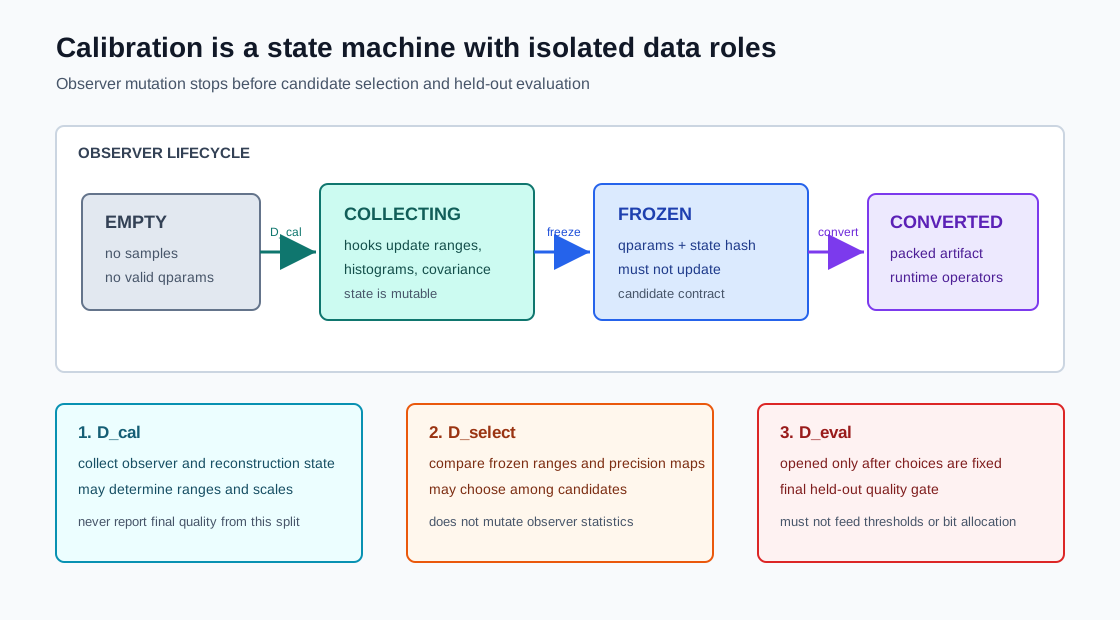
calibration:
    collect representative tensor or activation statistics
    and freeze numerical parameters

sensitivity analysis:
    estimate how much a candidate numerical change damages
    a local output or an end-to-end objective

precision allocation:
    choose one feasible option per module under a concrete
    memory, latency, energy, or artifact-size budget
These decisions are related, but they are not interchangeable. A percentile observer can choose a range without deciding a bit width. A layer scan can rank modules without producing a deployable graph. A mixed-precision optimizer can return a mathematically attractive map whose formats have no common runtime.
This article therefore owns the measurement and allocation layer between M8.1’s numerical representation and later M8 mechanisms. It preserves the full derivation and implementation path while deferring:
| Deferred mechanism | Owner |
|---|---|
| smoothing, rotations, and learned equivalent transforms | M8.3 |
| OBS/OBQ, GPTQ, and AWQ internal update rules | M8.4 |
| sparse exceptions, additive codebooks, and vector quantization | M8.5 |
| live activation and K/V scaling during serving | M8.6 |
| fake quantization, STEs, learned qparams, and QAT | M8.7 |
| native binary/ternary architecture and training | M8.8 |
| artifact conversion, packaging, loader, and kernel compatibility | M8.9 |
| deployment benchmarking, promotion, rollback, and release | M8.10 |
0x01 Calibration Is An Experiment, Not A Loader Loop
Calibration runs a reference model or selected operators over representative inputs while observers collect state. Post-training quantization keeps the model weights frozen; the state being fitted is numerical metadata or a reconstruction parameter, not a new model capability.
A defensible experiment separates fitting and selection from evidence about the chosen candidate. The protocol used here names five data roles; 0x06 explains their populations and independence rules:
| Dataset | Purpose | May influence quantization choices? |
|---|---|---|
| collect ranges, histograms, activations, or reconstruction state | yes | |
| compare candidate clipping methods or precision maps | yes | |
| confirm one frozen candidate on held-out examples from the declared calibration-fit population | no tuning; may block progression | |
| test that same candidate against preregistered distribution shifts and stress strata | no tuning; may block progression | |
| final held-out quality gate | no |
Reusing fitting or selection examples as supposedly independent confirmation or final evidence leaks feedback into the reported result. A good score can then reflect tuning to those examples rather than generalization. In particular, a selection score is not held-out confirmation merely because the observers never fitted those records.
Freezing a list of candidates is not enough if the final scores then choose a winner. Use to choose one candidate, including its precision map, clipping, correction rank/factor dtype, and runtime path. Before opening , freeze that candidate’s artifact and runtime identities and preregister the reference, metrics, thresholds, uncertainty procedure, and evaluation manifest. Final evaluation returns an acceptance or rejection receipt for that identity; it is not another ranking stage. This applies the official scikit-learn guidance on validation versus final test data to quantization search.
A failure is a valid result. Changing the candidate after seeing it requires a new identity and fresh independent release evidence under this single-use protocol; relabeling the same evaluation examples does not restore independence. An intentionally multi-candidate final audit instead needs candidate identities and the complete decision/inference rule preregistered together. It must not use their relative final scores to select or retune a winner. M8.10 owns the deployment release gate beyond this quality-evidence boundary.
The split must preserve preprocessing state as well as examples:
calibration manifest:
    source and revision fingerprints
    sample identifiers or hashes
    tokenizer and chat-template revision
    image/audio preprocessing revision
    truncation and padding rules
    sequence-length and modality buckets
    random seed and sampling weights
    observer configuration
    model revision and dtype
Weights are static, so plain per-tensor or per-channel MinMax weight quantization can be calibrated directly from the checkpoint. Activation quantization is data-dependent. Weight-only methods also become data-dependent when they minimize output reconstruction error, estimate curvature, or use activation magnitudes. weight-only does not imply data-free.
0x01A Requests And Tokens Define Different Workload Measures
Suppose request contains observed tokens and produces an error at token . A request-weighted objective is:
A token-weighted objective is:
The first gives each request equal influence. The second gives long requests more influence. Neither is universally correct; the serving objective must choose. A corpus with one very long document can dominate activation histograms even when most production requests are short.
0x01B Prompt Activations Are Not The Whole Decode Distribution
Teacher-forced prompts are convenient because many tokens can be processed in parallel. They may not reproduce activations created by generated prefixes during decode. A calibration plan should say which state it approximates:
prompt-only:
    inexpensive and stable, but may miss generated-prefix behavior

teacher-forced continuation:
    covers later positions without sampling drift

sampled decode traces:
    closer to serving state, but depends on decoding policy and seed

mixed phase corpus:
    explicit prompt/decode weights matching a target workload
M8.6 will own online activation and K/V quantization. M8.2 only establishes that the data used to freeze static parameters must match the state those parameters will see.
0x02 The Observer Is A State Machine
An observer is not merely a function that returns a scale. It is mutable state with a lifecycle:
EMPTY
  -> COLLECTING       observer hooks update statistics
  -> FROZEN           statistics and qparams stop changing
  -> CONVERTED        fake/reference operators become packed operators
Evaluation while observers are COLLECTING does not compare an immutable candidate: the numerical state can change during the evaluation. Such a run can still be replayable when the initial state, exact input order, batch/rank partition, merge order, update rule, randomness, software/hardware behavior, and evolving state snapshots are recorded; bitwise replay additionally depends on deterministic execution. Replayability is not evidence that qparams stayed fixed.
Candidate comparison on and final evidence on must use frozen observer/qparam snapshots with recorded identities, with observer updates disabled throughout scoring. Updating an observer after conversion changes the intended contract without rebuilding the packed artifact. Disabling observer updates is also distinct from disabling fake quantization: the candidate must still execute its intended numerical path. These are workflow requirements, not a claim that a PyTorch .eval() call freezes observers automatically.
0x02A Different Methods Need Different State
| Observer or calibrator | Stored state | Important behavior |
|---|---|---|
| MinMax | running minimum and maximum | extreme-value sensitive |
| moving-average MinMax | EMA minimum and maximum | order-dependent temporal estimator |
| percentile | samples, histogram, or quantile sketch | explicit tail clipping |
| histogram / entropy | bin counts, edges, min/max | threshold can be searched after collection |
| MSE range search | values or histogram sufficient to score candidates | objective matches element error |
| output reconstruction | input activations, covariance, or sampled rows | optimizes operator output rather than weights alone |
The PyTorch 2.8 moving-average observer (source pinned in the reference ledger below) updates the running minimum as:
and similarly for the maximum, where is the averaging constant. The first observed batch initializes the state. This is a temporal estimator, not a clipping objective: changing sample order can change the final range.
Renderer-safe update:
running_min = (1 - c) * running_min + c * batch_min
running_max = (1 - c) * running_max + c * batch_max
0x02B Shape Is Part Of Observer State
For , a per-tensor observer emits one scale. A per-channel observer may emit scales or scales depending on the selected axis. A grouped observer emits one scale per group.
The observer must record:
observed tensor name
logical shape and axis
group size G = values per group
number and shape of qparams
source dtype and device
collection phase
request, valid-token, scalar-value, group-update, and weight counters with units
range method and all hyperparameters
The G convention matches M8.1: larger means fewer metadata groups and coarser local adaptation.
0x02C Streaming Collection Trace
The accounting helper below is executable Python; the observer around it is framework-neutral pseudocode with method-specific statistics and immutable serialization supplied by adapters. This bounded example observes dense valid-token rows of width K, sharing one statistic per contiguous channel group across rows (axis=-1). Other axes, routed expert edges, and modalities need their own declared mapping; do not infer token count from a reshaped leading dimension.
Each input row is (request_id, values, token_weight). The hook must remove padded tokens before constructing rows. All retained weights must be finite and positive; zero-weight rows are excluded upstream. For request weighting, assign each token its request weight divided by the request’s total eligible token count, not the count in the current microbatch. Token weighting uses one per eligible token.
| Counter | Unit in this example |
|---|---|
request_count | distinct request IDs contributing at this edge, across calls |
token_count | valid token-observation events; repeated passes count again |
observed_value_count | scalar values actually observed, excluding token and group-tail padding |
group_update_count | nonempty persistent channel groups updated per call, summed over calls; changes with batching |
effective_sample_weight | sum of token weights once per token event, not once per channel/group; not statistical effective sample size |
For two requests contributing one and two tokens, width 5, and group size 2, one call gives 2 requests, 3 tokens, 15 values, and 3 group updates. Token weighting gives weight 3; equal request weighting gives 2. The short last group contains one real channel, not two padded values. A weighted histogram receives each scalar’s token weight; its per-group mass is consequently the token-weight sum times that group’s real width, not the ledger’s token mass.
from math import fsum, isfinite

def prepare_observation(rows, group_size):
    if type(group_size) is not int or group_size <= 0:
        raise ValueError("group_size must be a positive integer")
    rows = tuple((rid, tuple(values), float(weight))
                 for rid, values, weight in rows)
    if not rows:
        raise ValueError("no valid token observations")
    width = len(rows[0][1])
    for rid, values, weight in rows:
        if not isinstance(rid, str) or not rid or len(values) != width or not width:
            raise ValueError("stable request IDs and equal nonempty row widths required")
        if not isfinite(weight) or weight <= 0 or not all(map(isfinite, values)):
            raise ValueError("finite values and positive finite token weights required")
    mass = fsum(weight for _, _, weight in rows)
    if not isfinite(mass):
        raise ValueError("nonfinite token mass")
    groups = tuple(
        tuple((value, weight) for _, values, weight in rows
              for value in values[start:start + group_size])
        for start in range(0, width, group_size)
    )
    return groups, {
        "request_ids": frozenset(rid for rid, _, _ in rows),
        "token_count": len(rows),
        "observed_value_count": sum(len(values) for _, values, _ in rows),
        "group_update_count": len(groups),
        "effective_sample_weight": mass,
    }, width
class RangeObserver:
    def __init__(self, method, group_size):
        self.state = "EMPTY"
        self.method = method
        self.axis = -1
        self.group_size = group_size
        self.width = None
        self.request_ids = frozenset()
        self.counts = dict(token_count=0, observed_value_count=0,
                           group_update_count=0, effective_sample_weight=0.0)
        self.stats = initialize_stats(method, self.axis, group_size)

    def observe(self, rows):
        if self.state not in {"EMPTY", "COLLECTING"}:
            raise RuntimeError("observer updates are disabled")
        groups, ledger, width = prepare_observation(rows, self.group_size)
        if self.width is not None and width != self.width:
            raise ValueError("edge width changed")
        counts = {key: self.counts[key] + ledger[key] for key in self.counts}
        if not isfinite(counts["effective_sample_weight"]):
            raise ValueError("nonfinite cumulative token mass")
        # Adapter is pure: failure must not partially mutate existing statistics.
        stats = update_stats(self.method, self.stats, groups)
        self.stats, self.counts, self.width = stats, counts, width
        self.request_ids = self.request_ids | ledger["request_ids"]
        self.state = "COLLECTING"

    def freeze(self, bit_width, signed=True):
        if self.state != "COLLECTING":
            raise RuntimeError("freeze requires collected statistics")
        ranges = finalize_ranges(self.method, self.stats, bit_width)
        qparams = derive_qparams(ranges, bit_width, signed)
        # Immutable, detached serialization of stats, config, ledger and qparams.
        snapshot = immutable_snapshot(
            stats=self.stats, qparams=qparams,
            counts=dict(self.counts, request_count=len(self.request_ids)),
            request_ids=self.request_ids, width=self.width,
            method=self.method, axis=self.axis, group_size=self.group_size,
            bit_width=bit_width, signed=signed,
        )
        self.state = "FROZEN"
        return snapshot
An activation hook then has a narrow contract:
def calibration_hook(module_name, observer, inputs, output, batch_context):
    # Observe the exact tensor consumed by the future quantized boundary.
    x = select_quantized_boundary_tensor(inputs, output)
    rows = valid_token_rows(x.detach(), batch_context)
    observer.observe(rows)
Observing the output while later quantizing the input is a legal program and an invalid experiment. Module names alone are insufficient; the manifest must identify the exact tensor edge.
The valid_token_rows adapter binds request IDs, validity masks, token positions/collection passes, and weights to that exact edge. Repeated observations intentionally add token/value/weight mass again but do not add another distinct request; the manifest must disclose replays, deduplication, and pass multiplicity. MinMax ignores positive weight magnitude when taking extrema; a weighted histogram uses it, and an EMA needs its declared ordered update rule. The code does not pretend all methods implement one weighting algorithm. Hash the frozen serialization and bind it to the corpus, edge, configuration, and collection-order manifests. A hash detects changed bytes relative to a recorded identity; it is not an access-control mechanism.
0x02D Distributed Observers Need Merge Semantics
Independent ranks can merge MinMax state exactly:
Histograms can be summed only when their bin edges are identical. If each rank expands its own range, the counts refer to different intervals and require rebinning before reduction. Percentile sketches need a mergeable sketch algorithm or raw samples. EMA state is not commutative; averaging final EMAs does not reproduce one globally ordered stream.
def merge_observers(states):
    assert_same_method_axis_groups(states)
    if states[0].method == "minmax":
        return min(s.min for s in states), max(s.max for s in states)
    if states[0].method == "histogram":
        assert_identical_bin_edges(states)
        return sum_counts(states)
    raise NeedMethodSpecificMerge()
Merge the coverage ledger separately: union request IDs rather than adding distinct-request counts. Token/value/weight totals can be summed only for disjoint observation contributions; replicated tensor-parallel observations must not be counted as new samples. Group-update totals describe the actual rank-local updates, not the count of a hypothetical merged batch. Preserve rank partition and update order alongside the method-specific statistic.
0x03 Why Clipping Can Reduce Quantization Error
Use a signed symmetric -bit quantizer with:
and choose a positive clipping threshold . Its step size is:
The reconstructed value is:
For observed values , an empirical MSE calibrator solves:
where:
Split the samples by whether they lie inside the clipping range:
The second term is exact for symmetric saturation at . The first depends on the sample’s location relative to the integer grid.
Under the usual approximation that in-range rounding error is uniformly distributed in one step and endpoint effects are negligible:
so:
The first component generally grows as grows because every code step becomes wider. The second decreases because fewer values are clipped and clipped values travel a shorter distance. Their sum can have an interior minimum.
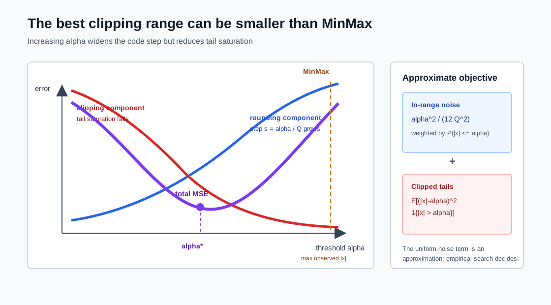
MinMax chooses:
It makes the empirical clipping term zero but does not minimize the total objective. One extreme value can enlarge the step for every other value in the group.
0x03A A Numeric Trace
Suppose an INT4 group has and mostly lies in , with one value at .
| Threshold | Step | Tail behavior |
|---|---|---|
| no clipping; ordinary values occupy only a few levels | ||
| the outlier clips by | ||
| fine ordinary resolution; the outlier clips by |
The best threshold depends on how many ordinary values exist, how important the outlier direction is, and which loss is measured. Counting only weight-element MSE can choose differently from measuring the layer output on real activations.
0x03B The Uniform-Noise Approximation Has Limits
The result is not a law for every tensor. It assumes approximately uniform phase within each quantization cell and ignores correlation, saturation boundaries, tiny samples, and discrete spikes. Transformer weights and activations can violate those assumptions. The empirical quantize-dequantize objective remains the final definition for an MSE search.
0x04 Range Selection Methods Are Different Estimators
The original quantization source A34 surveys MinMax, moving-average MinMax, percentile, entropy/KL, and MSE calibration. They should not be presented as equivalent names for clipping.
| Method | Decision rule | Main strength | Main failure mode |
|---|---|---|---|
| MinMax | include observed extrema | simple; no observed saturation | one outlier controls the step |
| moving-average MinMax | temporally smooth batch extrema | tracks drifting streams | order-dependent; may lag abrupt changes |
| percentile | retain a selected mass | explicit tail budget | percentile is workload- and tensor-dependent |
| MSE search | minimize empirical element reconstruction error | objective is direct and auditable | element MSE may not track model loss |
| entropy / KL | preserve a histogram distribution after quantization | distribution-aware | binning, smoothing, and expansion choices matter |
| ACIQ-style analytic clipping | derive threshold from a distributional error model | avoids an expensive threshold sweep | wrong distributional assumptions produce wrong thresholds |
0x04A Percentile Calibration
For symmetric clipping, percentile calibration can choose:
For asymmetric activations, lower and upper quantiles may be selected separately. 99.9% is not intrinsically safe: one tensor may have harmless noise in the final , while another stores rare but decisive routing or logit values there.
0x04B MSE Grid Search
def choose_mse_threshold(values, bit_width, candidates):
    qmax = 2 ** (bit_width - 1) - 1
    best = None
    for alpha in candidates:
        scale = alpha / qmax
        q = clamp(round(values / scale), -qmax, qmax)
        x_hat = scale * q
        loss = mean(square(values - x_hat))
        if best is None or loss < best.loss:
            best = Result(alpha=alpha, scale=scale, loss=loss)
    return best
Candidate thresholds may be quantiles, histogram edges, or a dense interval. The search report must record the grid; MSE calibrated is not enough to reproduce the result.
0x04C Histogram And Entropy Calibration
Let a histogram have counts and fixed edges . For each candidate threshold:
- choose the bins inside the candidate interval;
- fold clipped tail mass into boundary bins;
- map the retained bins into the available quantized bins;
- expand that compressed distribution back onto the reference-bin support;
- smooth zero-probability bins consistently;
- score the divergence between reference distribution and reconstructed distribution .
For KL divergence:
and the threshold is selected from the candidate with the smallest valid divergence.
def choose_entropy_threshold(hist, edges, quantized_bins):
    best = None
    for stop in candidate_end_bins(hist):
        p = fold_tail_into_boundary(hist, stop)
        q_small = merge_reference_bins(p, quantized_bins)
        q = expand_within_nonempty_bins(q_small, p)
        p_safe, q_safe = smooth_for_kl(p, q)
        score = kl_divergence(p_safe, q_safe)
        best = min_valid(best, Result(edges[stop], score))
    return best
There is no single implementation-independent histogram calibrator hidden behind the word entropy. Bin count, range expansion, tail folding, zero smoothing, and quantized-bin redistribution can change the result. ONNX Runtime exposes MinMax, Entropy, and Percentile as distinct static-calibration methods for this reason.
0x04D Static And Dynamic Range Selection
Static activation quantization freezes qparams from . Dynamic quantization computes at least some activation qparams at runtime from the current tensor.
| Choice | Benefit | Cost |
|---|---|---|
| static | stable artifact; qparams can be prepared ahead of the kernel | distribution shift can saturate or waste levels |
| dynamic | adapts to each live tensor or group | runtime reduction, synchronization, and scale-handling overhead |
Dynamic range computation can improve numerical fit and still lose latency. M8.6 will trace those runtime reductions in the activation and K/V paths.
0x05 Weight Error Becomes Activation-Weighted Output Error
Element MSE treats every weight coordinate equally. A linear operator does not.
Let:
and let a candidate quantizer reconstruct:
Then:
Therefore:
and the squared output error is:
Use cyclic invariance of the trace:
Define the calibration activation covariance-like matrix:
Then the error is weighted by the directions the workload actually activates:
Only when is this proportional to unweighted weight error:
Real Transformer activations are not generally isotropic. Two equal-norm weight perturbations can have very different output effects because one lies in a frequently activated direction.
This derivation is the bridge to activation-aware and second-order weight PTQ. M8.4 will derive how GPTQ and AWQ act on that information. M8.2 uses it to define what a calibration metric is actually measuring.
0x05A Quantizing Both Operands Adds Interaction Error
Let:
Then:
Expanding:
The first term is activation error through the original weight. The second is weight error under real activations. The third is an interaction term. Independent weight and activation scans can miss that interaction, especially at very low precision.
0x05B Reconstruction Metrics Answer Different Questions
| Metric | Formula or role | Blind spot |
|---|---|---|
| element MSE | ignores downstream geometry | |
| relative MSE | unstable near tiny reference outputs | |
| SQNR | compresses where error occurred into one number | |
| cosine similarity | output direction agreement | ignores magnitude error |
| max absolute error | worst observed element | highly sample-sensitive |
| task loss / perplexity | end-to-end behavior | expensive; can hide local regressions |
A serious calibration report stores local reconstruction and end-to-end quality. One is diagnostic; the other is the actual model contract.
0x05C ZeroQuant-V2: Quantization Error Can Have A Low-Rank Repair
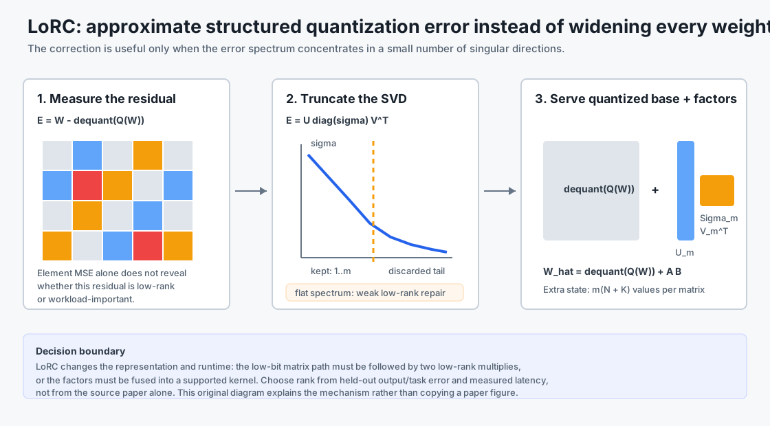
The activation-weighted derivation above asks how a weight residual affects real outputs. ZeroQuant-V2 adds a different question: after a low-bit quantizer has produced , is the remaining weight error structured enough to approximate with a small low-rank branch?
Define the dense residual:
Its singular value decomposition is:
The Eckart—Young theorem says the best rank- approximation under Frobenius norm keeps the first singular triplets:
Write the truncated product as two factors:
Then the corrected reconstruction is:
Renderer-safe form:
E = W - dequant(Q(W))
E_m = truncated_svd(E, rank=m) = A @ B
W_hat_lorc = dequant(Q(W)) + A @ B
The derivation explains both the opportunity and the limit. If contain most residual energy, a small branch can recover much of the Frobenius error. If the spectrum is flat, a low rank either leaves substantial residual or becomes too large to remain a useful compression.
0x05D Rate And Runtime Ledgers For The Repair
For , the correction stores:
values. If the factors use bits and the base codes plus metadata occupy bits, the first artifact ledger is:
The relative factor count compared with a dense matrix is:
For a square matrix with :
or about as many values as the dense matrix. At INT8 that is KiB of factor payload before scales and alignment. The base four-bit code payload is MiB, so the factor payload is small in storage terms. It is not free in execution.
For :
The correction adds approximately:
floating-point operations, two extra matrix multiplications, intermediate state , and possibly a second launch or fusion path. A low parameter ratio therefore does not prove low latency overhead. Decode with is especially sensitive to launch and metadata cost; prefill may amortize the branch differently.
def quantize_with_lorc(weight, quantizer, rank, factor_quantizer=None):
    qweight = quantizer.encode(weight)
    weight_q = quantizer.decode(qweight)
    residual = weight - weight_q

    U, sigma, Vh = truncated_svd(residual, rank=rank)
    A = U * sigma[None, :]
    B = Vh

    if factor_quantizer is not None:
        A = factor_quantizer.encode_with_qparams(A)
        B = factor_quantizer.encode_with_qparams(B)

    return qweight, A, B

def linear_lorc(x, qweight, A, B):
    y_base = low_bit_linear(x, qweight)
    y_repair = matmul(matmul(x, decode(B).T), decode(A).T)
    return y_base + y_repair
ZeroQuant-V2 reports using low ranks and quantized factors in its studied recipes. Those choices are source-reported, not universal constants. Rank, factor dtype, and eligible modules should be selected against held-out output/task error and the target runtime.
0x05E LoRC Optimizes A Different Objective Than Calibration Reconstruction
Truncated SVD minimizes:
The operator objective derived in 0x05 is instead:
These coincide only under an isotropic up to scale. A residual direction with modest singular value can matter greatly if production activations strongly excite it. Therefore a serious rank sweep records at least:
residual singular spectrum and retained Frobenius energy
held-out activation-weighted output error
end-to-end task deltas
factor payload and qparam bytes
prefill/decode latency with the actual correction kernel
modules where the correction is disabled or promoted to higher precision
The design alternatives are materially different:
| Response to difficult quantization error | Representation | Runtime path |
|---|---|---|
| raise base bit width | wider dense codes | one regular low-bit operator |
| LoRC | dense low-bit base plus dense low-rank correction | base operator plus two thin multiplies |
| sparse exceptions | low-bit base plus indexed high-precision values | dense path plus irregular sparse path |
| GPTQ-style compensation | change later weights during conversion | ordinary quantized operator after packing |
| learned transform | reshape error before quantization | fused transform or transform-aware operator |
LoRC belongs in M8.2 because the singular spectrum and activation-weighted validation are calibration evidence. The detailed extreme representations and exception paths remain in M8.5.
0x06 Representative Calibration Requires Coverage, Not Just Sample Count
A calibration set of 128 sequences is underspecified. Coverage depends on what those sequences contain and how activations are weighted.
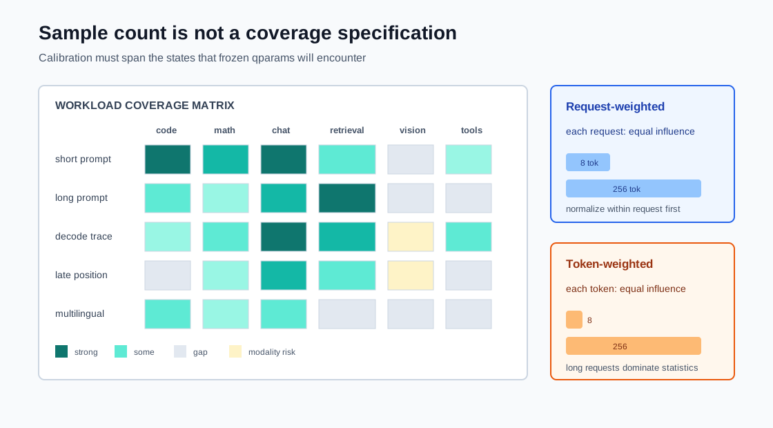
A useful coverage matrix can include:
| Axis | Example buckets |
|---|---|
| domain | code, math, retrieval, conversation, domain-specific text |
| language | languages or scripts present in production |
| context position | short, medium, long; early and late positions |
| generation phase | prompt prefill, teacher-forced continuation, sampled decode |
| modality | text, image tokens, audio tokens, projector outputs |
| template | system/user/assistant layouts and tool messages |
| routing | common and rare MoE expert paths, when observable |
LLMC’s benchmark analysis reports that calibration data, target bit widths, and algorithm choices all influence quantized quality. Its calibration experiments report benefits from aligning token distributions with the target data and preserving intra-sentence token order; the practical choice of domain coverage and corpus diversity remains a workload-specific design decision. That is evidence for an explicit corpus design, not permission to copy evaluation examples into calibration.
Data role and distribution are different labels. D_cal fits numerical state; D_select can guide repeated candidate comparisons. D_id and D_ood evaluate the one candidate chosen by that search, after its identity and their measurement/acceptance plan are frozen. D_eval remains sealed for the final quality gate. A selection set may itself contain both ordinary and shifted workloads; that does not make its reused scores independent ID/OOD confirmation.
Here, ID means held-out examples sampled from the declared calibration-fit population, with its stated domain, phase and weighting policy. OOD means a named departure from that population, not merely a new example and not “outside every possible future workload.” A shift can still lie inside the supported serving envelope. Conditions beyond the declared support envelope are exploratory stress tests and cannot silently become release requirements or a claim of supported operation. The broader need to evaluate declared distribution shifts is illustrated by WILDS; the five-role quantization protocol here is an article-level design, not a WILDS prescription.
For example, if the fit population is short English chat prefills, unseen short English chat prefills can provide ID confirmation. Long code contexts, late sampled-decode positions, or a different declared language mix can form separate OOD strata. Those labels would change if the fit population already included those conditions. Preregister the strata, reference model, metrics, weights, uncertainty treatment, and which checks are required before opening their results. Report each stratum’s evidence and missing coverage; an aggregate average cannot substitute for a required stratum, and neither an ID pass nor an OOD pass proves universal robustness.
These are logical evidence pools, not a requirement for five separate files. In this strict protocol, their examples are disjoint at a declared leakage unit: for example, keep a source document, conversation, and its derived chunks or augmentations in one role. Different row IDs or manifest hashes alone do not establish independence. Record the grouping/deduplication rule, role membership, distribution definition, access history, and candidate/plan identities. The counts in 0x02 describe observations at an edge; they do not prove dataset independence or coverage.
D_cal + D_select -> fit/search -> select and freeze candidate C
sealed D_id + D_ood -> preregistered confirmation of C, no candidate ranking
    required evidence missing or failed -> HOLD; leave D_eval sealed
    required checks satisfied -> admit C to its preregistered final quality gate
sealed D_eval -> acceptance/rejection receipt for C, not a new selection stage
An ID/OOD failure may diagnose a weakness and stop progression. If it prompts a change to clipping, precision, calibration data, runtime path, or the supported envelope, record a new candidate or plan identity. The exposed examples can become development evidence, but relabeling them does not make them fresh confirmation for the revised candidate. Keep the failed attempt, obtain fresh independent ID/OOD confirmation for any newly claimed results, and use final evidence untouched by that revision. A still-unopened final pool may remain reserved; an already exposed final pool cannot be reused under this article’s single-use rule. Merely choosing another frontier candidate after seeing confirmation results is selection too.
0x06A Multimodal Statistics Must Not Be Pooled Blindly
The applied module-wise mixed-precision article (Compression Series, part 8) and MBQ highlight a multimodal failure: vision and language tokens can have different sensitivity and magnitude distributions.
If one observer pools both modalities:
large-magnitude vision states can determine the shared scale
    -> language values receive coarse resolution

language-dominated sample counts can determine a clipping threshold
    -> rare visual states saturate
Possible designs include separate modality observers, modality-balanced reconstruction weights, or module-specific precision choices. The correct choice depends on whether the runtime can carry separate qparams and whether the model boundary identifies modalities at execution time.
0x06B Check Whether Statistics Have Stabilized
Collecting more tokens is useful only if it changes uncertainty. Compare qparams after and observations:
For many groups, report a distribution such as median, 95th percentile, and maximum . Histograms can also be compared by total variation, Jensen-Shannon divergence, or threshold drift, provided binning is stable.
for checkpoint in [n, 2*n, 4*n]:
    snapshot[checkpoint] = freeze_copy(observers)

for name in observers:
    drift = abs(scale[2*n][name] - scale[n][name]) / (
        abs(scale[n][name]) + eps
    )
    report_quantiles(name, drift)
Low average drift does not guarantee tail coverage. Report unstable modules and corpus strata, not only one global mean.
0x07 Sensitivity Is A Counterfactual Experiment
Calibration chooses numerical candidates. Sensitivity asks what happens if a candidate is applied to a particular module.
Let be a lower-is-better proxy or task loss for model . For module and precision option , an isolated scan defines:
where only module is changed.
reference = evaluate(model_fp, D_select)

for module in candidate_modules(model_fp):
    for option in feasible_options(module):
        candidate = replace_one_module(model_fp, module, option)
        local = reconstruction_metrics(candidate, module, D_cal)
        end_to_end = evaluate(candidate, D_select)
        record(module, option, local, end_to_end - reference)
        restore_reference_module(candidate, module)
This is not the same as starting from an all-low-precision model and restoring one module. The two baselines ask different questions:
| Scan | Question |
|---|---|
| quantize one module from FP | which isolated change is harmful? |
| restore one module from low precision | which repair helps this already-perturbed model? |
Interactions make the rankings differ.
0x07A Sensitivity Is Not Additive By Default
For two changes and , define:
If , the measured degradation is additive for that pair. If it is large, summing independent layer scores is a weak model of the combined artifact.
Testing every pair is usually too expensive. Practical searches can:
- compute isolated scores for all feasible module options;
- identify the highest-risk modules or tightly coupled blocks;
- measure selected pair interactions;
- solve an additive approximation;
- validate several candidates from the Pareto frontier end to end.
0x07B Magnitude, Empirical, And Curvature Scores
Sensitivity proxies form a spectrum:
| Proxy | State required | What it approximates |
|---|---|---|
| weight range or norm | checkpoint only | numerical difficulty, not model loss |
| activation magnitude | calibration forwards | how strongly input coordinates are used |
| local reconstruction | inputs and module outputs | operator-level output error |
| end-task scan | held-out proxy tasks | observed model degradation |
| Hessian/Fisher proxy | gradients, Hessian-vector products, or statistics | local loss curvature around the reference |
The second-order expansion for a perturbation is:
Near a stationary point, , leaving the curvature-weighted term. HAWQ uses Hessian information to rank layer sensitivity. HAWQ-V2 argues that one top eigenvalue does not represent the whole spectrum and uses average curvature through the Hessian trace.
If an isotropic approximation replaces by its average eigenvalue:
then for quantization perturbation :
This explains why a curvature score needs both sensitivity and the actual error introduced by a candidate quantizer. Curvature alone does not choose a format.
HAWQ-V2 estimates traces with stochastic methods such as Hutchinson estimation and selects mixed precision on a Pareto frontier. Its assumptions matter: a local expansion, approximately stationary parameters, and perturbations small enough for the quadratic model to remain useful. More generally, the article’s local Taylor model need not remain reliable when joint weight-and-activation low-bit perturbations are large. Empirical validation remains mandatory.
0x07C A Trace Estimator Is An Algorithm, Not A Label
For random vectors with :
An estimator is:
def hutchinson_trace(loss, params, probes):
    grad = autograd(loss, params, create_graph=True)
    estimates = []
    for _ in range(probes):
        v = rademacher_like(params)
        hv = autograd(dot(grad, v), params)
        estimates.append(dot(v, hv))
    return mean(estimates)
Probe distribution, probe count, objective batch, damping, and parameter partition all affect variance and cost. A report that says only Hessian-aware cannot be reproduced.
0x08 A Precision Map Is A Constrained Optimization Problem
Suppose module has feasible options . Introduce a binary decision:
with one option per module:
Let be an estimated degradation and a deployment cost. The additive allocation problem is:
subject to:
and compatibility constraints:
The cost must be named. Serialized bytes, loaded HBM, latency, energy, and conversion overhead are different objectives. M8.1 showed that a nominal bit width omits scales, zero-points, padding, and packing. A useful includes those terms and rejects unsupported kernel/layout combinations.
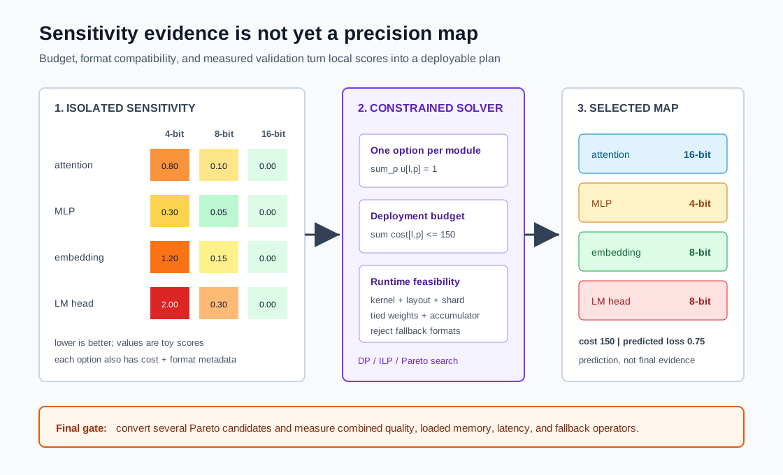
0x08A Dynamic Programming For One Additive Budget
After discretizing cost, a multiple-choice knapsack recurrence is:
def solve_precision_map(modules, options, budget):
    # dp[c] = (predicted degradation, selected options)
    dp = {0: (0.0, [])}
    for module in modules:
        next_dp = {}
        for used, (score, choices) in dp.items():
            for option in options[module]:
                if not runtime_feasible(module, option):
                    continue
                new_cost = used + option.cost
                if new_cost > budget:
                    continue
                candidate = (score + option.sensitivity,
                             choices + [(module, option)])
                next_dp[new_cost] = better(next_dp.get(new_cost), candidate)
        dp = pareto_prune(next_dp)
    return min(dp.items(), key=lambda item: item[1][0])
pareto_prune removes states that are both more expensive and more damaging than another state. The remaining states form predicted quality-cost candidates; several should be converted and measured because the additive model ignores interactions.
0x08B Toy Allocation Trace
Use normalized cost units, not claimed hardware measurements:
| Module | 4-bit (cost, sensitivity) | 8-bit | 16-bit |
|---|---|---|---|
| attention | (10, 0.80) | (20, 0.10) | (40, 0.00) |
| MLP | (30, 0.30) | (60, 0.05) | (120, 0.00) |
| embedding | (20, 1.20) | (40, 0.15) | (80, 0.00) |
| LM head | (20, 2.00) | (40, 0.30) | (80, 0.00) |
With budget , exhaustive evaluation of the assignments selects:
attention: 16-bit     cost 40   sensitivity 0.00
MLP:        4-bit     cost 30   sensitivity 0.30
embedding:  8-bit     cost 40   sensitivity 0.15
LM head:    8-bit     cost 40   sensitivity 0.30
------------------------------------------------
total                  150               0.75
The result is not keep the largest module in high precision and not rank modules by one sensitivity number. The selected upgrade depends on each option’s marginal quality gain per budget unit and on the alternatives available to every other module.
0x08C Multi-Objective Allocation
If cost has several dimensions:
one weighted scalar objective can hide unacceptable regressions. A deployment search is often clearer as constraints plus a Pareto set:
minimize quality degradation
subject to:
    loaded HBM <= B_memory
    p95 decode latency <= B_latency
    artifact size <= B_disk
    supported kernels only
Latency is not additive across modules when kernels overlap, batches change, or conversions force graph breaks. Use measured candidate latency for the final frontier, not only a sum of isolated microbenchmarks.
0x09 Runtime Feasibility Must Enter Before The Solver
A precision map is a graph plan, not a spreadsheet column.
0x09A Tied And Coupled Tensors
If the embedding and LM head share storage, assigning them different formats requires one of:
one shared representation
duplicate storage
runtime conversion
breaking the tie and accepting changed deployment semantics
The cost model must reflect the chosen path. Similar constraints appear when fused QKV projections, gated MLP pairs, or expert groups share a kernel layout.
0x09B Tensor Parallelism And Group Boundaries
Suppose a weight axis is sharded over ranks and quantization uses groups of values. A group crossing a shard boundary may require duplicated metadata, cross-rank preprocessing, or a different packing layout. Feasible options should validate:
def runtime_feasible(module, option):
    return all([
        kernel_registry.supports(module.op, option.format),
        option.group_axis in kernel_registry.axes(module.op),
        shard_layout_aligns(module.shape, option.group_size),
        accumulator_is_safe(module.shape, option),
        dtype_boundaries_are_supported(module, option),
        tied_weight_constraints_hold(module, option),
    ])
An option rejected here should not enter the mathematical optimizer. Otherwise the solver spends precision budget on a representation that will silently dequantize to BF16 or fall back to an unsupported slow path.
0x09C Conversion Boundaries Are Costs
A graph can mix INT8, INT4 weight-only, BF16, and FP8 operators. Every boundary may require dequantization, requantization, scaling, layout conversion, or a high-precision residual path.
operator format savings
    - metadata
    - padding
    - conversion kernels
    - unfused intermediate writes
    - duplicated tied tensors
    - fallback workspace
    = effective deployment benefit
Norms, small biases, embeddings, LM heads, routers, and multimodal projectors can have different sensitivity and kernel economics from dense Transformer matrices. Excluding a tiny tensor from low precision may cost little. Excluding a tied vocabulary matrix may cost a great deal.
0x0A End-To-End Calibration And Allocation Trace
The search below returns one frozen candidate, not final evaluation scores. These are framework-neutral orchestration contracts, not a drop-in quantization library. load_search_splits opens only calibration/selection records; split disjointness is checked from sealed manifests without exposing evaluation contents. measure_and_select_one uses the declared selection rule and , fails on an empty feasible frontier, and returns exactly one artifact.
def build_precision_candidate(model, manifests, runtime, budgets):
    assert_disjoint_manifest_ids(manifests)
    D_cal, D_select = load_search_splits(manifests)

    # 1. Register observers on exact graph edges.
    observers = register_observers(model, calibration_plan())

    # 2. Collect mutable statistics, then freeze a detached snapshot.
    with no_grad(), observers.collecting():
        for batch in D_cal:
            model(batch)
    observer_snapshot = observers.freeze()
    assert_collection_provenance(observer_snapshot, manifests.calibration)

    # 3. Finalize several range candidates, not one global default.
    qparam_candidates = {}
    for edge, state in observer_snapshot.items():
        qparam_candidates[edge] = [
            finalize_minmax(state),
            finalize_percentile(state, p=0.999),
            finalize_mse_search(state),
            finalize_entropy_search(state),
        ]

    # 4. Keep only options that have a real loader and kernel path.
    options = enumerate_format_and_qparam_options(model, qparam_candidates)
    options = runtime.feasibility_filter(options)

    # 5. Measure local and end-to-end sensitivity.
    scores = isolated_module_scan(model, options, D_cal, D_select)
    interactions = selected_pair_scans(model, scores.high_risk_pairs, D_select)

    # 6. Solve several budget points and export the Pareto candidates.
    maps = []
    for budget in budgets:
        maps.extend(solve_and_keep_frontier(scores, options, budget))

    artifacts = [runtime.convert(model, plan) for plan in maps]
    artifacts = [a for a in artifacts if runtime.smoke_test(a)]

    # 7. Selection remains on D_select, including combined-artifact checks.
    artifact = measure_and_select_one(artifacts, D_select, manifests.selection_rule)
    return freeze_release_candidate(
        artifact=artifact, observer_snapshot=observer_snapshot,
        runtime_manifest=runtime.manifest(), search_manifests=manifests,
    )
freeze_release_candidate binds immutable artifact bytes, precision/qparam/observer state, preprocessing, and the selected runtime configuration. The search does not open D_id, D_ood, or D_eval. Its manifest-disjointness contract covers all five roles, including the declared source-group leakage unit, not only the two pools it loads. Apply the 0x06 confirmation stage to this frozen candidate before final admission. Before opening final data, preregister a gate plan that binds this identity to an evaluation-manifest identity, fixed reference, metrics, thresholds, and uncertainty/decision rules, plus the required ID/OOD confirmation plan and receipts. The following low-level quality gate returns a receipt, never an alternative candidate:
def final_quality_gate(candidate, gate_plan, evaluation_vault):
    # candidate_identity accepts one frozen candidate, not a candidate list.
    identity = candidate_identity(candidate)
    if identity != gate_plan.candidate_identity:
        raise ValueError("candidate differs from preregistered identity")
    plan_hash = hash_gate_plan(gate_plan)
    D_eval = evaluation_vault.open_once(gate_plan, plan_hash)
    metrics = evaluate_fixed_candidate(candidate, D_eval, gate_plan)
    if candidate_identity(candidate) != identity or hash_gate_plan(gate_plan) != plan_hash:
        raise RuntimeError("candidate or gate plan changed during evaluation")
    return acceptance_receipt(identity, plan_hash, metrics, gate_plan)
The vault is a durable evaluation-access boundary: it verifies the registered plan and dataset identity, prevents reuse across process restarts or candidate changes, and marks the manifest consumed before exposing records. Before that access, its admission adapter must also require the plan’s ID/OOD receipts to match the exact candidate, confirmation plan and role manifests, with every required check satisfied; missing, failed, stale or incomplete evidence leaves final data sealed. It is not just an in-memory boolean or a filename. acceptance_receipt applies the already fixed acceptance rule and records pass/fail, measured results, candidate/plan/data identities, and reference identity; missing/nonfinite required results fail closed. No failed gate falls back to the next frontier candidate on the same final set. Recovery or changes require fresh independent release evidence. For intentionally preregistered multi-candidate audits, use the separate joint protocol described in 0x01, not a loop around this single-candidate gate.
Identity checks alone cannot prevent evaluation leakage or transient mutation that is later restored. The adapters must enforce immutable candidate/plan access, disabled observer updates, controlled data access, and an append-only attempt record. This trace specifies and tests the orchestration boundary; it does not implement production access control, a statistical inference engine, conversion kernels, or M8.10’s deployment release machinery.
In a large model, holding a complete model copy per scan is wasteful. A practical implementation swaps or quantizes one module in place, clears temporary buffers, restores the reference state, and checks a checksum after every trial.
reference_hash = hash_parameters(model)
for trial in trials:
    with temporary_module_replacement(model, trial.module, trial.quantized):
        score(trial)
    assert hash_parameters(model) == reference_hash
This assertion catches cumulative quantization, failed restoration, and accidental in-place modification of the reference weights.
0x0B Design And Paper Variants
The methods in this article answer different parts of the pipeline:
| Method or lineage | Range/data decision | Sensitivity decision | Precision decision | Important distinction |
|---|---|---|---|---|
| MinMax | observed extrema | none | fixed externally | preserves observed range, not total MSE |
| percentile | empirical tail mass | none | fixed externally | clipping budget is explicit |
| entropy/KL | histogram distribution | none | fixed externally | minimizes a distribution divergence |
| ACIQ | analytic distribution model | none | fixed externally | depends on a fitted distributional assumption |
| local reconstruction | calibration inputs/outputs | measured operator error | can feed a solver | activation-weighted, but still local |
| HAWQ | calibration loss/curvature | top Hessian eigenvalue | mixed precision | one dominant curvature direction |
| HAWQ-V2 | calibration loss/curvature | average Hessian trace plus perturbation | Pareto allocation | uses more of the Hessian spectrum |
| LLMC/QBench framing | algorithm- and data-dependent | magnitude or Hessian families | evaluates many schemes | emphasizes calibration and runtime variance |
| MBQ | modality-balanced calibration | modality-specific reconstruction sensitivity | can guide mixed precision | vision and language tokens need not be equally sensitive |
| ZeroQuant-V2 LoRC | quantization residual plus rank sweep | residual spectrum and held-out reconstruction | low-bit base plus low-rank correction | Frobenius-optimal rank is not automatically workload-optimal |
0x0B1 What Training Does And Does Not Happen Here
The baseline M8.2 workflow is PTQ:
base weights: frozen
optimizer state: none
gradients: optional only for curvature/Fisher measurement
learned model update: none
fitted state: ranges, scales, clipping parameters, precision map
Some advanced PTQ methods optimize clipping or equivalent-transform parameters on calibration data. That is still not ordinary model fine-tuning, but it introduces an optimizer, stopping rule, and overfitting risk. M8.3 covers learned transforms; M8.7 covers quantization-aware training where model parameters are trained under fake or real low-precision constraints.
0x0C Reproducibility Record
A publishable calibration record should be sufficient to regenerate the numerical plan:
model:
  revision: exact-checkpoint-id
  reference_dtype: bf16

data:
  calibration_manifest: sha256:...
  selection_manifest: sha256:...
  id_confirmation_manifest: sha256:...
  ood_stress_manifest: sha256:...
  evaluation_manifest: sha256:...
  calibration_fit_population: sha256:...
  supported_serving_envelope: sha256:...
  id_sampling_and_weighting: sha256:...
  ood_strata_metrics_weights_and_required_checks: sha256:...
  disjointness_unit: source_group_including_derived_examples
  role_membership_and_deduplication: sha256:...
  access_and_candidate_attempt_history: sha256:...
  tokenizer_revision: ...
  chat_template_revision: ...
  weighting: request_weighted
  prompt_decode_mix: [0.7, 0.3]

confirmation:
  candidate_artifact_and_runtime_hash: sha256:...
  preregistered_plan_hash: sha256:...
  reference_identity: sha256:...
  id_receipt: sha256:...
  ood_per_stratum_receipts: sha256:...
  retuning_policy: exposed_data_becomes_development_not_fresh_confirmation

observer:
  edge: blocks.0.mlp.down_proj:input
  method: histogram_mse
  bins: 2048
  axis: -1
  group_size: 128
  ledger: # example only; counts and weights come from this exact edge
    request_count: 128
    token_count: 131072
    observed_value_count: 536870912 # 131072 valid tokens * width 4096
    group_update_count: 4096 # 128 update calls * 32 persistent channel groups
    effective_sample_weight: 128.0 # one total weight per request, one pass
    units: distinct_requests_valid_token_events_scalar_values_group_calls_token_mass
  width: 4096
  update_calls: 128
  padding: excluded_before_observation
  replay_policy: one_pass_no_repeated_token_observations
  collection_order_and_rank_partition: sha256:...
  frozen_state_hash: sha256:...
  frozen_qparams_hash: sha256:...

search:
  metrics: [relative_mse, sqnr, proxy_loss]
  precision_options: [int4_g128, int8_channel, bf16]
  budget_type: loaded_bytes
  interaction_pairs: ...

runtime:
  engine_version: ...
  hardware: ...
  supported_kernel_manifest: sha256:...

final_quality_gate:
  candidate_artifact_and_runtime_hash: sha256:...
  preregistered_plan_hash: sha256:...
  reference_identity: sha256:...
  metrics_thresholds_and_uncertainty_rule: sha256:...
  evaluation_manifest: sha256:...
  confirmation_plan_hash: sha256:...
  required_confirmation_receipts: [sha256:id_receipt, sha256:ood_receipts]
  confirmation_admission: exact_candidate_plan_role_manifests_all_required_checks
  missing_or_failed_confirmation: hold_without_opening_final_data
  evaluation_access: sealed_until_candidate_and_plan_frozen
  retry_policy: new_candidate_requires_fresh_independent_release_evidence
Seeds alone do not reproduce a corpus whose source changed. Names such as C4 calibration do not reproduce filtering, tokenization, lengths, or sample weights.
0x0D Failure Lab
| Failure | Observable symptom | Root cause | Required check |
|---|---|---|---|
| evaluation leakage | excellent proxy score, weak independent result | influenced thresholds or map | disjoint manifests plus candidate/plan freeze before final access |
| final-set winner selection | best-looking frontier candidate becomes the release candidate | final scores became another selection objective | select one on the selection split; final gate returns only its acceptance receipt |
| selection relabeled as confirmation | apparently independent ID/OOD success after repeated tuning | exposed examples reused under a new role name | role access history and fresh confirmation after retuning |
| aggregate hides missing stress coverage | mean score passes while a required workload stratum is absent or fails | distribution labels and required checks were not bound to the plan | per-stratum receipts; missing/failed required evidence keeps the final pool sealed |
| stale observer update | repeated conversion changes scales | observer remained in collecting state | lifecycle assertion and state hash |
| replay mistaken for frozen evaluation | deterministic rerun but qparams change while scoring | repeatable update history confused with fixed numerical state | disabled updates and frozen snapshot identity throughout comparison |
| ambiguous calibration count | changing group size appears to change corpus size | reshaped leading dimension labeled as samples | separate request/token/value/group/weight ledger with explicit mask and replay rules |
| wrong tensor edge | plausible qparams, severe runtime error | observer watched output instead of quantized input | graph-edge manifest and hook test |
| one outlier owns MinMax | ordinary values collapse into few codes | no clipping search | histogram and threshold sweep |
| percentile copied globally | isolated modules regress | tail importance differs by tensor | per-module candidate comparison |
| distributed histogram mismatch | rank-count-dependent thresholds | unequal bin edges were summed | common edges or explicit rebin |
| calibration corpus imbalance | one domain/modality works, another collapses | sample counts do not match workload | coverage matrix and weighted metrics |
| additive sensitivity failure | predicted map is good, combined artifact is bad | module interactions | pair scans and frontier validation |
| Hessian proxy overconfidence | curvature rank disagrees with measured loss | quadratic/local assumptions fail | empirical candidate conversion |
| nominal-bit cost model | artifact exceeds memory budget | metadata, padding, or duplication omitted | M8.1 effective-size ledger |
| unsupported precision option | no speedup or hidden BF16 fallback | solver ignored kernel registry | feasibility filter and loaded-op trace |
| tied-weight disagreement | artifact duplicates a large matrix | two formats assigned to shared storage | tie constraint before optimization |
| prompt-only activation range | long decode saturates | generated-prefix state absent | prompt/decode calibration mix |
| LoRC rank selected only by retained singular energy | good weight MSE, weak output/task recovery | workload covariance differs from Frobenius geometry | activation-weighted and end-to-end rank sweep |
| low-rank factors omitted from runtime budget | artifact looks small, decode regresses | two thin multiplies and launch/fusion cost ignored | factor bytes, intermediate shape, prefill/decode timing |
| factor dtype changed after rank selection | unexplained quality loss | SVD factors were evaluated in FP but served quantized | decode factors exactly as deployed during selection |
Calibration can also reveal a limit of threshold tuning: at a fixed bit width and sharing domain, keeping an extreme channel can make the grid too coarse for ordinary values, while clipping it can remove useful signal. M8.3 takes the next step by changing coordinates rather than only the range, using equivalent transforms that preserve the pre-quantization function in exact arithmetic. The transformed graph still needs calibration and error checks; equivalence before quantization does not guarantee better low-bit accuracy.
0x0E Boundaries And Handoffs
M8.2 produces:
frozen observer state
candidate qparams and clipping methods
local and end-to-end sensitivity evidence
interaction warnings
runtime-feasible precision-map candidates
calibration, selection, ID/OOD confirmation, and reserved final-data role manifests
candidate-bound ID/OOD receipts when confirmation has been performed
It does not claim that those candidates are released artifacts.
| Next article | What it receives from M8.2 |
|---|---|
| M8.3 | observed outlier distributions, activation directions, and modules where clipping alone fails |
| M8.4 | calibration activations/covariance and scalar weight-only baselines |
| M8.5 | sensitivity evidence for nonuniform or exception-based representations |
| M8.6 | phase- and workload-specific activation/KV statistics |
| M8.7 | reference qparams and modules that need QAT rather than PTQ |
| M8.8 | PTQ/QAT baselines for comparison with native binary/ternary training |
| M8.9 | frozen precision-map candidates and manifests for conversion and loader validation |
| M8.10 | calibration/selection provenance, sensitivity evidence, candidate-bound ID/OOD confirmation evidence, and reserved final-data identity for deployment release gates |
0x0F Claim Status
| Claim | Status |
|---|---|
| A34 presents MinMax, moving-average MinMax, percentile, entropy/KL, and MSE calibration families. | Source-local |
| Static activation calibration and dynamic runtime qparam computation have different overhead contracts. | Source-local / externally verified by ONNX Runtime documentation |
| PyTorch moving-average MinMax uses an exponential update of running extrema. | Externally verified by official PyTorch documentation |
| ACIQ derives clipping from an analytic quantization-error model under distributional assumptions. | Externally verified by the ACIQ paper |
| HAWQ uses Hessian information; HAWQ-V2 replaces a top-eigenvalue view with average trace-based sensitivity and Pareto selection. | Externally verified by the HAWQ and HAWQ-V2 papers |
| Calibration choice, calibration data, target bits, and runtime support materially affect LLM quantization outcomes. | Externally verified by LLMC/QBench |
| ZeroQuant-V2 studies low-rank compensation of the residual between original and quantized weights and reports that activation quantization sensitivity varies by model family and scale. | Externally verified by ZeroQuant-V2 |
| Vision and language tokens can exhibit different quantization sensitivity. | Externally verified by MBQ |
| The clipping decomposition and activation-weighted linear-output derivation in this article follow from the stated quantizer and linear algebra. | Rewrite derivation |
| The precision-map toy costs and sensitivities are pedagogical normalized units, not measured deployment results. | Rewrite interpretation |
| The five data roles, strict disjointness rule and confirmation-before-final-admission workflow are the protocol used in this article, not a universal requirement for five physical datasets. | Article-level design; ID/OOD claims are limited to declared populations and strata |
| An additive layer-sensitivity solver predicts the final combined loss exactly. | False in general; interactions require validation |
0x10 Publish Gate
- Calibration, selection, and final evaluation data are distinct; one candidate and its acceptance plan are frozen before final access.
- Observer replayability is distinguished from immutable comparison, and counter units, shape, lifecycle, merge semantics, and freezing are explicit.
- The clipping objective is derived into rounding and saturation terms.
- MinMax, EMA, percentile, MSE, entropy, and analytic clipping are compared as different methods.
- Weight MSE is connected to activation-weighted output reconstruction by derivation.
- Joint weight/activation error includes the interaction term.
- Quantization-residual SVD is derived into a low-rank correction, with storage, FLOP, factor-dtype, and workload-weighted validation boundaries.
- Corpus coverage includes request/token weighting, prompt/decode state, and modalities; ID/OOD confirmation is separated from selection, with population definitions, retuning history and final-admission rules.
- Empirical, magnitude, reconstruction, and Hessian sensitivity alternatives are separated.
- HAWQ and HAWQ-V2 assumptions and differences are stated.
- Mixed precision is formulated as constrained optimization with a worked solution.
- Kernel, layout, tied-weight, sharding, and conversion feasibility enter before allocation.
- PTQ fitting is distinguished from QAT and model fine-tuning.
- Later M8 mechanisms retain clear ownership.
0xFF References
Local Series Sources
- Transformer Series (34) - Quantitative Fundamentals - calibration methods, granularity, static/dynamic quantization, PTQ, and QAT.
[SOURCE-LOCAL] - Transformer Series (35) - Fundamentals of Large Model Quantization - LLM weight/activation behavior, outliers, and quantization method boundaries.
[SOURCE-LOCAL] - Transformer Series (36) - Large Model Quantization Scheme - activation-aware, curvature-aware, mixed-precision, and learned-calibration methods.
[SOURCE-LOCAL] - Compression Series (8) - Fixed-Base Multimodal PTQ and Module-Wise Mixed Precision - applied precision matrix, module scans, multimodal calibration, and runtime evidence.
[SOURCE-LOCAL] - M8.1 - Quantized Numbers and the Kernel Contract - representation, qparam shape, packing, accumulator, and effective-size contract.
[TRANSFORMER SYSTEM]
Primary Papers And Official Documentation
- Post Training 4-bit Quantization of Convolutional Networks for Rapid-Deployment - ACIQ analytic clipping and clipping/noise tradeoff; arXiv v3.
[PAPER] - HAWQ: Hessian AWare Quantization of Neural Networks With Mixed-Precision - Hessian-aware layer sensitivity and mixed precision; arXiv v1.
[PAPER] - HAWQ-V2: Hessian Aware Trace-Weighted Quantization of Neural Networks - average Hessian trace, perturbation-aware scoring, and Pareto precision selection; arXiv v1.
[PAPER] - ZeroQuant-V2: Exploring Post-training Quantization in LLMs from Comprehensive Study to Low Rank Compensation - LLM PTQ sensitivity study and low-rank compensation of quantization residuals; arXiv v3.
[PAPER, SOURCE-REPORTED RECIPES] - LLMC: Benchmarking Large Language Model Quantization With a Versatile Compression Toolkit - calibration data, method families, sensitivity choices, and runtime-aware LLM quantization evaluation; arXiv v3, not a pin of the toolkit’s current code.
[PAPER] - MBQ: Modality-Balanced Quantization for Large Vision-Language Models - modality-dependent sensitivity and balanced reconstruction; CVPR 2025 open-access proceedings, pp. 4167–4177; method sections also inspected in author arXiv v2. The proceedings PDF retrieval failed; no byte identity with that PDF is claimed.
[PAPER] - PyTorch 2.8 MovingAverageMinMaxObserver - official EMA observer update; exact implementation identity is recorded below.
[OFFICIAL-DOC / VERSION-SPECIFIC] - PyTorch 2.8 Quantization API Reference and disable_observer - observer, histogram, fake-quantization and observer-control APIs.
[OFFICIAL-DOC / VERSION-SPECIFIC] - ONNX Runtime Quantize ONNX Models — pinned documentation source - static/dynamic quantization and MinMax, Entropy, and Percentile calibration examples; documentation and runtime revisions are distinct below.
[OFFICIAL-DOC / REVISION-SPECIFIC] - scikit-learn 1.7: Cross-validation and final evaluation - model selection can leak test-set information; validation and final test roles differ. The single-use candidate/plan protocol here is an article-level design, not a scikit-learn API.
[OFFICIAL-DOC / WORKFLOW APPLICATION] - WILDS: A Benchmark of in-the-Wild Distribution Shifts - ICML 2021, PMLR 139, pp. 5637–5664; primary-source background on evaluating explicitly defined distribution shifts, not a quantization benchmark or evidence that this article’s candidate passes its stress matrix.
[PAPER / CONCEPTUAL BACKGROUND]
Source-Version Ledger
All references above were accessed on 2026-09-29. The arXiv links select explicit paper revisions; MBQ and WILDS select named proceedings editions. The implementation entries below select checked evidence baselines, not the latest release or a deployment recommendation. A versioned documentation URL can still be rebuilt; commit links identify the implementation or documentation source independently.
-
PyTorch observer and fake-quantization APIs. Checked docs: 2.8; release:
v2.8.0; commit:ba56102387ef. Sources: observer.py, fake_quantize.py. Accessed: 2026-09-29.Scope:
torch.aoobserver/fake-quantizer behavior; no packed backend or device qualification. Claim anchors: 0x02–0x02A (EMA initialization/update and separate observer/fake-quant controls), 0x04 (observer families). -
ONNX Runtime documentation. Checked documentation snapshot:
935a9bbd79e2; source: quantization.md. This is not a versioned runtime manual. Accessed: 2026-09-29.Scope: general workflow description; no execution-provider support claim. Claim anchors: 0x04A/0x04C/0x04D (named calibration methods and the static/dynamic distinction).
-
ONNX Runtime quantization tooling. Checked release:
v1.22.0; commit:f217402897f4. Sources: calibrate.py, quantize.py. Accessed: 2026-09-29.Scope: Python calibration/conversion interfaces; no CPU, CUDA or TensorRT provider qualified by this citation. Claim anchors: 0x04A/0x04C (MinMax, Entropy and Percentile are supported examples, not an exhaustive enumeration), 0x04D (static/dynamic entry points).
-
scikit-learn evaluation guidance. Checked docs: 1.7 reporting 1.7.2; release:
1.7.2; commit:25dee604bae1. Source: cross_validation.rst. Accessed: 2026-09-29.Scope: evaluation methodology; no inference backend. Claim anchor: 0x01 (tuning versus final test); the five-role/single-use protocol remains this article’s design.
These pins record evidence used by the article; deployment eligibility still binds the actual runtime/build, execution provider, hardware and artifact through M8.9/M8.10. The ONNX documentation snapshot is not asserted to be the documentation build for v1.22.0; the two sources were checked separately for the limited claims listed. Pinning a source does not execute its implementation, reproduce its benchmarks, or make every linked subpage part of this evidence baseline.