M8.4 - Scalar Weight-Only PTQ: RTN, GPTQ, and AWQ
0x00 Why Weight-Only PTQ Became The Practical LLM Baseline
The first deployment target for large-model quantization is often not integer-only inference. It is a mixed operator: weights are stored at low bit width, activations remain FP16 or BF16, and a specialized kernel reconstructs weight tiles close to the multiply-accumulate units.
That choice follows from the shape of autoregressive inference. During low-batch decode, every generated token reuses the model weights while processing only a small number of activation rows. Moving the weight matrices can dominate the local linear-layer cost, so reducing their bytes can matter even when unpacking and dequantization add arithmetic. During large prefill, the same operator can become more compute-heavy and the tradeoff can change. Weight-only PTQ is therefore a workload-shaped baseline, not a universal theorem that activations should remain high precision.
It became attractive for three practical reasons:
- weights are fixed and available offline, so conversion can be completed before serving;
- no new full training run is required, which matters for models whose original data or compute budget is unavailable;
- W4A16-style kernels can preserve the existing floating activation and residual interfaces while reducing the largest static payload.
The weakness is equally important: once the original training is over, PTQ must approximate a function it cannot retrain. The converter can choose scales, codes, order, equivalent transforms, and local compensation, but it cannot freely reorganize the learned representation.
0x00A From Independent Rounding To Output Reconstruction
Round-to-nearest is the natural starting point. With a fixed scalar grid, it minimizes the squared error of each weight independently. But a linear layer is not consumed one scalar at a time. It is consumed as , and calibration inputs can make two equally large weight errors have very different output consequences.
This gap connects modern LLM PTQ to an older second-order lineage:
| Method idea | Question it asks | What it contributes to M8.4 |
|---|---|---|
| magnitude or RTN | which local scalar/grid point is closest? | independent baseline |
| Optimal Brain Damage | which parameter has low second-order loss importance under a diagonal approximation? | curvature-aware importance |
| Optimal Brain Surgeon | how should remaining parameters compensate after one parameter is constrained? | inverse-curvature compensation |
| Optimal Brain Quantization | how should a weight be quantized and the remaining row updated? | greedy PTQ formulation |
| GPTQ | how can that compensation be made tractable for very large Transformer matrices? | common ordering, damping, Cholesky state, lazy block updates |
| AWQ | can activation evidence protect salient channels through equivalent scaling rather than second-order reconstruction? | activation-aware alternative |
The progression is not a simple sequence where each method strictly replaces the previous one. RTN is cheap and can be strong at moderate precision. GPTQ spends calibration memory and conversion work to preserve layer outputs. AWQ avoids backpropagation and full reconstruction while searching channel scales and clipping choices. Their assumptions, conversion costs, and runtime artifacts differ.
0x00B “Weight-Only” Describes The Served Operand, Not The Evidence
A weight-only artifact stores low-bit weights while keeping live activations at higher precision. The converter may still depend heavily on activations:
RTN:
    can be data-free once group ranges are chosen

GPTQ:
    collects calibration inputs to build X^T X
    and minimize layer-output reconstruction

AWQ:
    uses activation statistics to identify and protect salient channels
The label therefore describes which operand is quantized in the runtime operator, not whether the conversion used data. This distinction is essential when reproducing a result: calibration corpus, sequence length, preprocessing, activation collection point, and block order are part of the method state.
0x00C Conversion Quality And Runtime Quality Are Separate
A fake-quantized matrix can show excellent reconstruction while producing no deployment benefit. The runtime still needs a physical packing, scale layout, zero-point convention, tile shape, and kernel. Group size may help numerical quality while increasing metadata or preventing a fast kernel. Activation ordering may help GPTQ while requiring a stored permutation. An asymmetric zero-point may improve range fit while adding correction work.
The complete comparison must therefore cross three gates:
- conversion: were codes and compensation computed according to the intended algorithm?
- artifact: do packed codes and metadata reconstruct the same ?
- execution: does the admitted kernel consume that representation without hidden dequantization or fallback?
0x00D Choosing Codes Is An Optimization Problem
M8.1 derived affine quantization, grouping, metadata, packing, accumulation, and the kernel contract. M8.2 built the calibration experiment and precision map. M8.3 showed how equivalent transforms can change quantization difficulty before any code is selected.
The next question is narrower and deeper:
Given a scalar low-bit grid and calibration inputs, how should a weight-only post-training quantizer choose codes, compensate for rounding error, and emit an artifact that a real W4A16 kernel can consume?
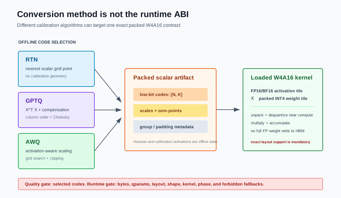
The baseline is round-to-nearest, or RTN. It assigns every weight to its nearest grid point under an independent scalar error. GPTQ instead measures the layer-output error induced by calibration activations and updates still-unquantized weights to compensate for each decision. AWQ uses the same activation evidence differently: it searches an equivalent per-input-channel scaling that protects salient channels before ordinary group quantization.
Those are conversion algorithms. They are not inference ABIs.
conversion method:
    RTN, GPTQ, or AWQ decides which low-bit values should represent W

runtime artifact:
    packed codes + scales + zero-points + group/layout metadata

runtime operator:
    high-precision activation x packed low-bit weight
    with fused unpack/dequantize/multiply/accumulate

quality and speed are separate gates:
    a better reconstruction solver does not guarantee a supported fast kernel
This article owns ordinary scalar weight-only PTQ:
| Owned here | Deferred owner |
|---|---|
| fixed scalar grids, RTN, OBD/OBS/OBQ lineage, GPTQ, AWQ | M8.4 |
| sparse high-precision exceptions, nonuniform scalar codebooks, additive quantizers, incoherence processing, vector quantization | M8.5 |
| request-dependent activation and K/V quantization | M8.6 |
| QAT, fake quantization, STEs, learned qparams, and distillation | M8.7 |
| native binary/ternary architecture and training | M8.8 |
| conversion manifests, loader compatibility, and executable kernels | M8.9 |
| deployment benchmark matrix, release, and rollback | M8.10 |
M8.4’s executable scope is a method-local scalar PTQ fixture. Freezing, packing and reopening its selected codes is necessary evidence, not generic artifact admission: M8.9 owns reusable containers, bounded loading, compatibility, topology, security and fallback across representation families.
The local A35/A36 articles provide the historical and method spine. The derivations and implementation contracts below are checked against Optimal Brain Compression, GPTQ, AWQ, and their official repositories. Where the local source calls GPTQ’s matrix a full model-loss Hessian, this article tightens the claim: for the linear-layer reconstruction objective used here, the curvature matrix is induced by the calibration inputs.
0x01 The Weight-Only Operator And Artifact
Use the same row-major convention as M8.1-M8.3:
is the number of token rows processed by the local operator, is the input/reduction dimension, and is the output dimension. Weight-only quantization keeps in FP16 or BF16 and stores an approximation through low-bit scalar codes.
For a group of weights, an affine representation stores:
The mathematical approximation is:
A practical kernel should not materialize the full in HBM before every multiplication. It reads packed codes and their group metadata, unpacks and dequantizes tiles near the compute units, multiplies them by high-precision activation tiles, and accumulates in a supported type.
0x01A Size Ledger
For -bit codes and groups along :
If every group stores one -byte scale and one -byte zero-point:
The real artifact also contains padding, alignment, tensor headers, possible permutations, and packing-layout overhead:
For , INT4 codes occupy:
With , FP16 scales, and one byte per zero-point, there are
groups and roughly KiB of scale/zero-point payload. This is only a representation ledger. It says nothing about whether the target kernel accepts the zero-point convention, scale ordering, packing permutation, or padded shape.
0x01B Method Name Is Not A File Format
GPTQ model and AWQ model are common labels, but neither name fully specifies an executable artifact. A loader still needs:
bit width and signed/unsigned code convention
group axis and group size
scale and zero-point dtype
original tensor shape and padding
packed nibble/bit ordering
weight transpose convention
optional input-column permutation
kernel family and supported activation dtype
tensor-parallel shard convention
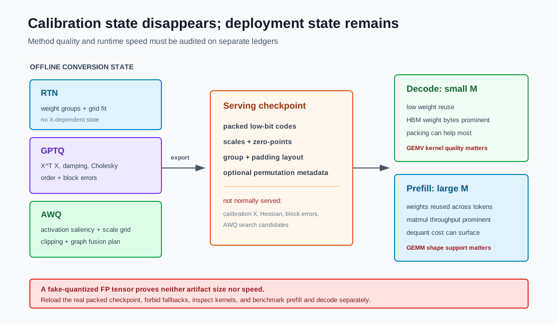
The conversion algorithm may disappear completely after export. GPTQ’s Hessian/Cholesky state and AWQ’s calibration activations do not belong in the serving checkpoint unless a tool explicitly stores them for reproducibility.
0x02 RTN: The Independent Scalar Baseline
Assume the scale and zero-point are fixed and clipping does not activate. A code reconstructs to . Under scalar squared error, the best integer code solves:
Divide by :
The nearest integer to minimizes that distance, so:
Clipping projects that integer onto the legal code interval. RTN is therefore not arbitrary: it is the exact optimizer of an independent scalar squared-error problem on a fixed grid.
Renderer-safe derivation:
minimize over integer q:
    (w - s * (q - z))^2

equivalent because s^2 > 0:
    (w / s + z - q)^2

solution:
    q = nearest_integer(w / s + z), then clip to code range
0x02A What RTN Does Not Optimize
RTN minimizes each weight’s local error. A layer is evaluated through calibration inputs:
These objectives coincide only in special geometries. Let . Then:
If , the input channels are isotropic under the calibration sample and output error is proportional to weight MSE:
If channel energies differ or channels are correlated, the same scalar weight error can have very different output impact.
Consider two possible error vectors:
Both have weight MSE . If
then:
The first rounding error is one hundred times more damaging to the calibrated layer output. GPTQ and AWQ both use activation evidence to address this mismatch, but by different mechanisms.
0x02B Group RTN Tensor Trace
Let one weight row be:
with and an unsigned 2-bit affine code range . Each consecutive group receives its own range and grid.
For group 0, :
For group 1, :
The second group spends much of its grid on the 3.1 outlier. Changing changes both the grid and metadata count. It is not merely an implementation tiling knob.
def group_rtn(weight, bits, group_size, asymmetric=True):
    # weight: [N, K]; groups are consecutive slices of K.
    N, K = weight.shape
    codes = empty_uint_storage(N, K, bits)
    qparams = []

    for n in range(N):
        for g0 in range(0, K, group_size):
            g1 = min(g0 + group_size, K)
            values = weight[n, g0:g1]
            scale, zero = choose_affine_grid(values, bits, asymmetric)
            q = round(values / scale) + zero
            q = clamp(q, code_min(bits, asymmetric),
                         code_max(bits, asymmetric))
            codes[n, g0:g1] = q
            qparams.append((n, g0 // group_size, scale, zero))

    return pack_codes(codes, bits), pack_qparams(qparams)
RTN remains the essential baseline. If a sophisticated calibrated method cannot beat it on held-out quality under the same grid and runtime format, the extra conversion state is not justified.
0x03 Calibration Inputs Define Reconstruction Geometry
For one output row , the reference output over calibration tokens is . Let be its quantized approximation. The row reconstruction loss is:
Expand the squared norm:
Define:
Then:
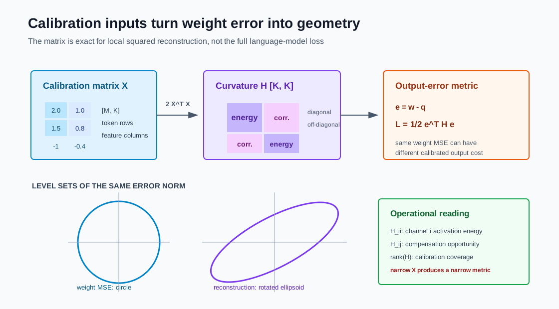
This is exact curvature for the stated linear-layer squared reconstruction objective. It is positive semidefinite and depends only on layer inputs, not on the output row. It is not the exact Hessian of the full language-model training loss.
For the full matrix:
Every output row is an independent optimization problem, but every row shares the same curvature matrix. That fact is the scalability hinge used by GPTQ.
0x03A What The Matrix Means
The diagonal records channel energy:
The off-diagonal entries record empirical channel correlation:
If is diagonal, one weight error cannot be compensated by another coordinate under this metric. If is large, changing coordinate can offset some output effect of an error at coordinate .
0x03B Streaming Curvature Collection
The complete calibration activation matrix need not remain resident. For batches :
If the objective is the average over token rows, normalize by . Multiplying by a positive scalar does not change the ideal compensation direction, but it changes absolute loss values and interacts with damping conventions. The manifest must record the convention.
class ReconstructionState:
    def __init__(self, in_features, device):
        self.gram = zeros([in_features, in_features], fp32, device)
        self.token_rows = 0

    def observe(self, x):
        # x: [..., K]. Masks must remove padding/non-data rows first.
        x2 = select_calibration_rows(x).reshape(-1, x.shape[-1]).float()
        if not isfinite(x2).all():
            raise ValueError("nonfinite calibration rows")
        self.gram += x2.T @ x2
        self.token_rows += x2.shape[0]

    def hessian(self):
        if self.token_rows == 0:
            raise ValueError("no valid calibration token rows")
        return 2.0 * self.gram / self.token_rows
An empty or completely masked calibration stream is an error, not an all-zero curvature estimate. Valid observed rows whose values are all zero are a distinct case: they count as observations and trigger the declared unseen-channel policy below. Collection must reject nonfinite inputs before accumulation.
For , a dense FP32 requires MiB per active layer. Layer-at-a-time conversion can reuse that storage. Capturing all layer Hessians simultaneously would multiply the memory burden.
0x03C Calibration Is Part Of The Method
comes from a chosen corpus, tokenizer, chat template, sequence-length distribution, and layer execution order. A narrow sample induces a narrow metric. The required state includes:
source model and tokenizer revision
calibration sample hashes
attention/padding mask policy
number of contributing token rows
layer input edge and shape convention
H normalization and accumulation dtype
damping policy
quantizer grid specification
held-out selection/evaluation split
M8.2’s calibration discipline still applies. A second-order-looking method can overfit just as easily as a clipping sweep.
0x04 OBD, OBS, And OBQ: From Importance To Compensation
The historical lineage matters because each step removes one simplifying assumption.
| Method | Forced change | Curvature used | Compensation? |
|---|---|---|---|
| OBD | set a weight to zero | diagonal approximation | no |
| OBS | set a weight to zero | full local inverse Hessian | yes |
| OBQ | move a weight to a scalar grid point | full layer-reconstruction inverse Hessian | yes |
| GPTQ | same scalar-grid problem | shared input-induced curvature and fixed column order | yes, made scalable |
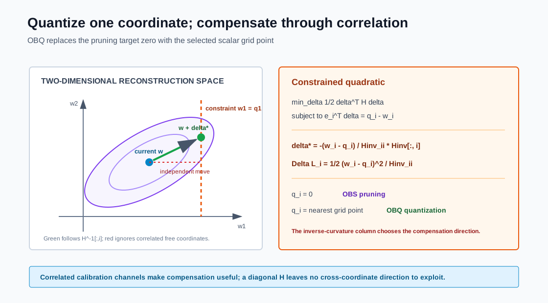
OBD approximates the loss increase of deleting as under a diagonal independence assumption. OBS keeps interactions and asks how all remaining coordinates should move when coordinate is constrained. OBQ changes the constraint target from zero to the selected quantization point.
0x04A Deriving The Constrained Update
Let be the current row and let be the grid value chosen for coordinate . We seek a perturbation minimizing the quadratic reconstruction increase while enforcing:
Equivalently:
where is the -th canonical basis vector. The constrained problem is:
Form the Lagrangian:
Stationarity with respect to gives:
so:
Apply the constraint:
Therefore:
and the optimal compensating update is:
The -th component is:
so the constrained coordinate lands exactly on .
Substitute into the quadratic:
This is the OBQ greedy score. The numerator is scalar rounding error. The denominator changes its functional cost through calibration geometry.
Renderer-safe result:
constraint:
    w[i] + delta[i] = q[i]

optimal compensation:
    delta = -(w[i] - q[i]) / Hinv[i,i] * Hinv[:,i]

loss increase:
    0.5 * (w[i] - q[i])^2 / Hinv[i,i]

pruning is the special case q[i] = 0
0x04B Removing A Fixed Coordinate
After coordinate is quantized, it is no longer available for future compensation. Let be the remaining indices. The inverse curvature for the reduced system can be updated by a rank-one downdate:
This is a Schur-complement/Gaussian-elimination relation. It avoids recomputing an inverse from scratch at every decision, but OBQ still chooses a potentially different greedy coordinate order for every output row. That row-specific order is expensive at LLM scale.
0x05 OBQ Compensation Trace
Consider:
and a weight row:
on the binary grid . Suppose the first coordinate is quantized to . Its scalar error is:
The optimal update is:
The first coordinate becomes exactly 1 and the second moves from to :
The compensation is not a heuristic transfer of raw error. Its direction is the corresponding inverse-curvature column.
If independent RTN quantizes the original row, the result is . Its error vector is and its quadratic loss is:
After compensation, the adjusted second coordinate rounds to 0, producing . Relative to the original row, the error is :
Under ordinary unweighted squared error, looks better: versus . Under the calibrated output geometry, the compensated solution is better. That is the entire reason to carry into scalar code selection.
0x05A Why Exact OBQ Does Not Scale Directly
For every output row, exact greedy OBQ repeatedly:
scores every still-free coordinate
chooses the row-specific minimum-loss coordinate
quantizes it
updates all remaining weights
downdates the row's inverse curvature state
For , the row-specific ordering leads to roughly cubic dependence on for every row. The GPTQ paper characterizes OBQ’s cost as for a matrix. Even a vectorized implementation is too expensive for billions of weights.
GPTQ’s central approximation is not ignore curvature. It is give every row the same column order, which lets every row share the same sequence of reduced curvature states.
0x06 GPTQ Step 1: A Common Column Order
The GPTQ paper reports that, especially for large heavily parameterized layers, greedy OBQ order provides only a small improvement over an arbitrary fixed order. GPTQ therefore quantizes all output rows in the same input-column order.
Because depends only on :
same input X
    -> same H for every output row

same column order
    -> same remaining-coordinate set at every step

same remaining-coordinate set
    -> same reduced inverse-curvature state for every row

result
    -> quantize the entire W[:, i] column in parallel
This changes the dominant complexity from row-specific cubic work toward:
where covers the curvature factorization and covers matrix-wide compensation. Constants, batching, and memory traffic still matter.
The approximation is a design tradeoff:
| Choice | Accuracy pressure | Conversion pressure |
|---|---|---|
| exact row-specific greedy OBQ | locally best next coordinate per row | prohibitive ordering/state work |
| natural fixed order | no saliency sort | common state and simple export |
| activation order | high- columns first | permutation and group-layout implications |
The official GPTQ repository later added act-order, which sorts columns by decreasing diagonal curvature/activation magnitude. It also added static-groups, which determines group grids before permutation so act-order need not require an inference-time layout change. Those are implementation variants, not part of the single sentence GPTQ uses Hessians.
0x07 GPTQ Step 2: Damping And Cholesky State
may be singular because calibration inputs do not span all directions. It can also be ill-conditioned. GPTQ adds diagonal damping:
The original implementation sets:
with a default percdamp of . This is a source implementation choice, not a universal optimum.
If a diagonal entry is exactly zero, the reference code marks the channel as dead, sets the corresponding diagonal to one for factorization, and zeroes the associated weight column. A production implementation must verify that the channel is truly unseen under valid masks rather than accidentally excluded by calibration preprocessing.
0x07A Why Cholesky Appears
Repeated inverse downdates can accumulate numerical error. GPTQ precomputes the required information more stably:
L = cholesky(H_d)                  # H_d = L @ L.T
Hinv = cholesky_inverse(L)         # H_d^-1
R = cholesky(Hinv, upper=True)     # H_d^-1 = R.T @ R
The sequential implementation uses rows of the upper-triangular . Let and let the current weight column be . After quantizing it to :
The working weights from column onward are updated by:
At column itself:
The update therefore both fixes the current column and propagates a curvature-shaped correction to future columns.
Do not substitute for in this factorized algorithm. is a Cholesky-factor diagonal. The earlier OBQ equation and this implementation are related formulations with different stored state.
0x08 GPTQ Step 3: Lazy Block Updates
A naive implementation updates the full trailing weight region after every quantized column. That performs little arithmetic per byte moved and becomes bandwidth-bound during conversion.
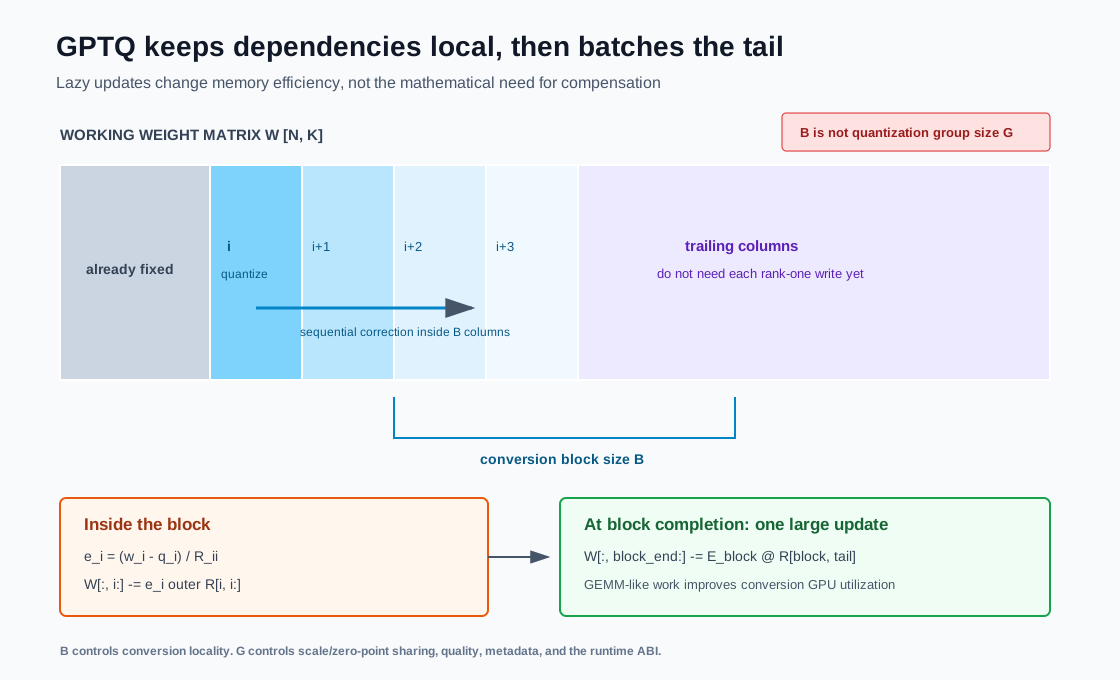
GPTQ processes a conversion block of columns. Inside the block, updates remain sequential because a column’s final rounding decision depends on corrections from earlier columns. The update to columns beyond the block can wait. Once the block is complete, all trailing corrections are applied as one matrix multiplication.
For block indices , collect scaled errors:
The delayed trailing update is:
This does not remove the theoretical arithmetic. It turns many memory-inefficient rank-one updates into a larger GEMM-like operation.
0x08A Block Size Is Not Group Size
Two frequently confused parameters live on different contracts:
| Parameter | Meaning | Survives into runtime artifact? |
|---|---|---|
GPTQ blocksize | how many columns share a lazy conversion update | usually no |
quantization groupsize | how many weights share scale/zero-point metadata | yes |
and can be chosen simultaneously, but equality is incidental. Changing mainly changes conversion memory locality and temporary state. Changing changes quantization grids, quality, metadata, and kernel compatibility.
0x08B Detailed GPTQ Pseudocode
def current_compensated_slice(W, W_block, E_block, R,
                              i0, i1, start, stop):
    # start is inside [i0, i1); do not mutate the delayed tail in W.
    group = W[:, start:stop].clone()
    inside_end = min(stop, i1)
    group[:, :inside_end - start] = W_block[:, start - i0:inside_end - i0]
    if stop > i1:
        # Earlier decisions in this block have not yet reached W[:, i1:].
        group[:, i1 - start:] -= E_block[:, :start - i0] @ R[i0:start, i1:stop]
    return group


def gptq_quantize_linear(W, calibration_batches, qspec,
                         block_size=128, damp_percent=0.01,
                         act_order=False, static_groups=False):
    # W: [N, K]. Activations remain high precision at inference.
    N, K = W.shape
    if min(N, K, block_size, qspec.group_size) <= 0:
        raise ValueError("nonempty matrix and positive block/group sizes required")
    if not isfinite(damp_percent) or damp_percent < 0:
        raise ValueError("finite nonnegative damping required")
    W = W.float().clone()  # Private conversion state; do not alter the source.
    if not isfinite(W).all():
        raise ValueError("nonfinite weights")

    # 1. Collect the layer-reconstruction curvature in FP32.
    H = zeros([K, K], fp32, W.device)
    token_rows = 0
    for X in calibration_batches:
        X = select_valid_rows(X).reshape(-1, K).float()
        if not isfinite(X).all():
            raise ValueError("nonfinite calibration rows")
        H += 2.0 * (X.T @ X)
        token_rows += X.shape[0]
    if token_rows == 0:
        raise ValueError("no valid calibration token rows")
    H /= token_rows

    # 2. Handle unseen channels and choose an optional common order.
    dead = diag(H) == 0
    H[dead, dead] = 1
    W[:, dead] = 0

    original_group_grids = None
    if static_groups:
        original_group_grids = [
            freeze_grid(g) for g in fit_all_group_grids(W, qspec)
        ]

    perm = arange(K)
    if act_order:
        perm = argsort(diag(H), descending=True)
        W = W[:, perm]
        H = H[perm][:, perm]

    # 3. Dampen and build a stable upper Cholesky factor of H^-1.
    damp = damp_percent * mean(diag(H))
    H += damp * eye(K)
    L = cholesky(H)
    Hinv = cholesky_inverse(L)
    R = cholesky(Hinv, upper=True)

    Q = zeros_like(W)
    codes = zeros_like(W, dtype=int64)
    group_index = zeros([K], int64, W.device)
    grids = original_group_grids if static_groups else []
    active_grid = None
    active_group = None
    for i0 in range(0, K, block_size):
        i1 = min(i0 + block_size, K)
        W_block = W[:, i0:i1].clone()
        E_block = zeros_like(W_block)
        R_block = R[i0:i1, i0:i1]

        # Sequential dependency remains inside the block.
        for j in range(i1 - i0):
            global_col = i0 + j
            w = W_block[:, j]

            if static_groups:
                # Map a permuted processing column back to its original group.
                original_col = perm[global_col] if act_order else global_col
                active_group = int(original_col) // qspec.group_size
                grid = grids[active_group]
            elif starts_new_quant_group(global_col, qspec.group_size):
                group_end = min(global_col + qspec.group_size, K)
                # Include pending in-block errors even beyond the block edge.
                current_group = current_compensated_slice(
                    W, W_block, E_block, R, i0, i1, global_col, group_end
                )
                active_grid = freeze_grid(fit_group_grid(current_group, qspec))
                active_group = len(grids)
                grids.append(active_grid)
                grid = active_grid
            else:
                grid = active_grid

            assert grid is not None
            code = encode_column(w, grid)
            q = decode_column(code, grid)
            d = R_block[j, j]
            scaled_error = (w - q) / d

            Q[:, global_col] = q
            codes[:, global_col] = code
            group_index[global_col] = active_group
            E_block[:, j] = scaled_error
            W_block[:, j:] -= outer(scaled_error, R_block[j, j:])

        # One matrix update carries the whole block's errors to the tail.
        W[:, i1:] -= E_block @ R[i0:i1, i1:]

    if act_order:
        inverse = inverse_permutation(perm)
        Q, codes = Q[:, inverse], codes[:, inverse]
        group_index = group_index[inverse]

    artifact = pack_exact_scalar_artifact(
        codes=codes, grids=grids, group_index=group_index, qspec=qspec,
        processing_permutation=perm,
        grouping_mode="original_columns" if static_groups else "processing_order",
    )
    assert_exact_scalar_fields(artifact, codes, grids, group_index)
    assert_close(decode_scalar_artifact(artifact), Q, rtol=0, atol=0)
    return artifact
current_compensated_slice constructs a temporary fully compensated group. The
active portion comes from W_block; a tail crossing i1 also needs the pending
earlier-column errors before its grid is fitted. It does not write that correction
back early, which would apply it twice at block closure. This matters for, e.g.,
block_size=3, group_size=2, not only aligned defaults.
freeze_grid copies the final qparams in their declared storage precision;
encode_column and decode_column consume those exact values and M8.1’s ordered
round/clip rules. The packer may change physical layout, never fit new grids.
Codes, qparams and original-column-to-group mapping survive conversion. Dynamic
groups follow processing order, so undoing act-order need not restore contiguous
original-column groups; a runtime must support that mapping or reject it.
assert_exact_scalar_fields compares unpacked codes, qparam bytes/dtypes and group
identity, not only floating reconstruction: coincident grids must not silently
erase the declared metadata contract.
For example, selected two-bit codes [0,2] with s=1,z=1 decode to [-1,1].
Refitting those endpoints with s=2/3,z=2 gives codes [0,3] and reconstruction
[-4/3,2/3]: exporting a dequantized matrix is not exporting the selected artifact.
The factorized loop is a teaching contract inspired by the
pinned GPTQ implementation,
with explicit artifact preservation and unaligned-group handling; it is not a
claim that every GPTQ converter implements this generalized interface.
0x09 GPTQ Integration Choices
The algorithm is only one layer of the conversion pipeline.
0x09A Layer-At-A-Time Execution
A memory-conscious converter typically:
- loads one Transformer block or target linear layer on the accelerator;
- replays cached block inputs or runs calibration samples through it;
- collects each target layer’s input statistics;
- quantizes target modules in a defined order;
- runs the quantized block to produce inputs for the next block if sequential reconstruction is enabled;
- writes packed artifacts and releases temporary curvature state.
true-sequential in the official GPTQ repository performs sequential quantization even within one Transformer block. Later sublayers then see activations produced by already-quantized earlier sublayers rather than only pristine reference activations. This can better match accumulated deployment error, but makes module ordering and activation recapture part of the method.
0x09B Natural Order, Act-Order, And Static Groups
act-order sorts input columns by decreasing . Intuitively, high-energy columns are quantized while many free coordinates remain available for compensation. But permutation interacts with grouping:
dynamic groups after permutation:
    group membership follows processing order
    selected grids may not map to consecutive original columns
    runtime may need permutation-aware metadata or input rearrangement

static groups:
    fit grids on original consecutive groups first
    process columns in act-order using their original group's grid
    undo column permutation in exported W
    runtime can keep ordinary original-order input layout
The official repository states that static groups let act-order avoid inference changes. Exact behavior remains implementation-specific; the artifact manifest must record whether any permutation survived export.
0x09C Grid Choice Is Orthogonal To Compensation
GPTQ is often associated with asymmetric group quantization, but the reconstruction algorithm does not mathematically require one universal affine convention. The quantizer can use a symmetric or asymmetric fixed grid, different group sizes, and different bit widths if the implementation and runtime agree.
This distinction matters when comparing results:
GPTQ compensation quality
    cannot be isolated if bit width, group size, clipping, and grid convention also change

runtime speed
    cannot be attributed to GPTQ if packed layout or kernel family also changes
0x09D Conversion-State Ledger
For one layer, representative temporary state is:
| State | Shape | Purpose |
|---|---|---|
| working weights | compensated full-precision values during conversion | |
| curvature | calibration reconstruction metric | |
| Cholesky/inverse factor | stable update rows | |
| output codes/dequantized | selected scalar points | |
| block errors | lazy trailing update | |
| qparams | runtime group grids |
The objects can be substantial but do not scale with . The working matrices dominate for wide output layers. Layer streaming and host/device offload policy must be designed, not assumed.
0x0A AWQ: Activation Saliency Without Curvature Compensation
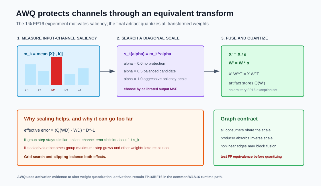
AWQ starts from a diagnostic experiment. It reports that preserving a small fraction of weight channels in FP16 can dramatically improve low-bit quality when those channels are selected by activation magnitude, while selecting by weight magnitude or randomly is much less effective in the studied models.
That experiment does not define the final deployable format. A scattered FP16 exception path is hardware-inefficient. AWQ converts the activation-awareness observation into a per-input-channel equivalent scaling, quantizes all weights, and avoids the mixed-precision exception artifact.
For input channel , define a calibration saliency proxy:
Large means the corresponding weight column repeatedly multiplies larger activation values under the calibration distribution. It does not prove semantic importance for every request, but it is a stronger output-error proxy than weight magnitude alone.
0x0AA Equivalent Channel Scaling
Let:
Define:
Then:
The floating-point function is identical. Quantize only the transformed weights:
Subtract the reference output:
For channel , the transformed weight quantization error is divided by when viewed in the original function. If scaling a salient column by does not materially enlarge its group’s quantization step, its effective error can shrink roughly in proportion to .
The condition matters. Group quantization shares a range. A large scale can create a new group maximum, enlarge the step, and damage nonsalient weights. AWQ therefore searches a balanced scale rather than sending salient channels toward infinity.
0x0AB The AWQ Search Space
AWQ parameterizes per-channel scales from activation magnitudes with one scalar exponent:
Implementations may normalize the resulting vector to control overall scale magnitude; that normalization and the exact module handler belong in the implementation manifest.
For each candidate , evaluate the quantized transformed layer under calibration inputs:
is a small grid. There is no gradient through the integer quantizer and no base-weight retraining. AWQ still uses output reconstruction as a deterministic selection score; no backpropagation or regression should not be misread as no calibration output comparison.
Renderer-safe objective:
saliency[k] = mean_over_calibration(abs(X[:, k]))
scale[k]    = max(saliency[k], eps)^alpha

choose alpha by grid search to minimize:
    || X W^T - (X / scale) Q(W * scale)^T ||_F^2
0x0AC Why The 1% FP16 Result Is Not The AWQ Artifact
The AWQ paper uses a 0.1%-1% high-precision-channel experiment to establish the saliency principle. The deployment method replaces that irregular mixed-precision representation with scaling followed by full low-bit quantization.
| Stage | Purpose | Runtime representation |
|---|---|---|
| FP16 salient-channel ablation | demonstrate which channels matter | diagnostic only |
| activation-aware scale search | protect salient channels while considering others | calibration state |
| transformed full-weight quantization | produce regular low-bit groups | packed scalar codes |
Saying AWQ stores 1% of weights in FP16 confuses the motivating ablation with the final method.
0x0B AWQ Scale, Clipping, And Graph Fusion
The scale search is architecture-aware because one activation edge can feed several linear layers. If a normalized hidden state feeds , , and projections, the inverse activation scaling must be consistent across those consumers. If a scale is absorbed into a preceding normalization, its affine parameters must be updated consistently.
Representative flow:
def search_awq_scale(x, linears, qspec, alpha_grid):
    # x: [M, K], linears share the same input edge.
    reference = {name: x @ layer.weight.T
                 for name, layer in linears.items()}
    saliency = mean(abs(x), dim=0).clamp_min(1e-5)

    best = None
    for alpha in alpha_grid:
        scale = normalize_scale(saliency.pow(alpha))
        x_scaled = x / scale
        error = 0.0

        for name, layer in linears.items():
            w_scaled = layer.weight * scale[None, :]
            w_q = pseudo_group_quantize(w_scaled, qspec)
            y_q = x_scaled @ w_q.T
            error += mse(y_q, reference[name])

        if best is None or error < best.error:
            best = SearchResult(alpha, scale, error)

    return best
The selected transform is then applied to the graph:
def apply_awq_scale(producer, consumers, scale):
    # Exact rewrite before weight quantization.
    absorb_inverse_scale_into_producer(producer, scale)
    for linear in consumers:
        linear.weight *= scale[None, :]
Whether producer is a LayerNorm, RMSNorm, activation wrapper, or another linear edge depends on the architecture. Some nonlinear boundaries prevent complete fusion and require a runtime scale operation. The original AWQ implementation includes model-specific handlers for attention and MLP structures; a generic converter must not infer graph legality from matching tensor dimensions alone.
0x0B1 Clipping Search
After scaling, AWQ can search a clipping ratio for each group or channel block. Let be the maximum absolute transformed weight in group and a clipping ratio:
The candidate grid is built from or the selected asymmetric range. Smaller sacrifices extreme values but decreases the quantization step for ordinary values. The search evaluates MSE under the exact qspec.
Clipping and scaling interact:
scale search changes which values define each group range
clipping search changes the range after scaling
group size determines which values compete for that range
zero-point convention changes the representable grid
The order used by a specific implementation must be preserved during export. Re-running a generic min/max quantizer after applying cached AWQ scales can discard the clipping decision.
0x0B2 Search State, Fake Quantization, Real Packing
The official AWQ repository exposes the deployment stages explicitly:
1. run AWQ search and save scale/clipping results
2. load search state and evaluate with fake/pseudo quantization
3. generate real packed INT4 weights
4. load the packed model through the real backend
The fake-quantized model uses floating tensors containing quantized-dequantized values. It validates numerical quality but does not prove memory reduction or kernel speed. Only the real packed artifact can exercise the actual loader and W4A16 kernel.
0x0B3 AWQ And SmoothQuant Are Related, Not Identical
Both use an exact diagonal transform, but their owner objectives differ:
| Property | SmoothQuant | AWQ |
|---|---|---|
| primary deployment target | weight-and-activation quantization, commonly W8A8 | weight-only low bit, commonly W4A16/W3A16 |
| pressure being moved | activation outlier range into weights | protect activation-salient weight columns |
| scale proxy | activation and weight maxima with migration parameter | activation magnitude with searched exponent |
| online activations | quantized in target W8A8 path | remain FP16/BF16 in target W4A16 path |
| article owner | M8.3 geometry | M8.4 scalar weight code selection |
The algebra overlaps. The calibration objective and runtime contract do not.
0x0C RTN, GPTQ, And AWQ Compared Mechanistically
| Dimension | RTN | GPTQ | AWQ |
|---|---|---|---|
| activation evidence | none required for code selection | full reconstruction geometry | per-channel activation saliency plus output score |
| core action | independently choose nearest grid point | quantize a column and compensate future columns | equivalently rescale input channels, then quantize |
| sequential dependency | none | yes, within processing order | scale/clipping search by module group |
| second-order state | none | dense curvature/factor | none |
| backpropagation | no | no | no |
| base-weight retraining | no | no | no |
| conversion cost | low | high | moderate search cost |
| graph rewrite | not inherently | permutation may matter; usually no functional graph transform | equivalent scale absorption is required |
| typical runtime artifact | packed scalar codes and qparams | packed scalar codes and qparams | packed scalar codes and qparams after scale fusion |
| main failure mode | ignores activation geometry | narrow/ill-conditioned calibration and incorrect sequential/export state | saliency/scale overfit or illegal graph fusion |
These methods are not mutually exclusive at the level of ideas. An exporter could apply an equivalent transform and then use a curvature-aware solver on the transformed weights. But the combined method must be evaluated as a new pipeline: calibration state, group grids, compensation geometry, and runtime layout all change. This article does not claim that an arbitrary AWQ-plus-GPTQ composition is paper-equivalent to either original method.
0x0C1 Decision Rules
RTN is defensible when:
the target bit width/group size already passes quality
calibration data is unavailable or legally constrained
conversion simplicity and reproducibility dominate
the runtime grid differs from calibrated tools' supported grids
GPTQ is attractive when:
low-bit scalar weight error needs explicit correlation-aware compensation
representative layer inputs can be collected
conversion time and KxK state are acceptable
the exact exported grouping/permutation has a supported kernel
AWQ is attractive when:
activation saliency is concentrated by input channel
an equivalent scale can be fused legally through the model graph
a small deterministic search is preferable to dense curvature state
the runtime supports the resulting packed W3/W4 group format
The final choice belongs to a Pareto comparison under identical qspec, calibration/evaluation split, and runtime.
0x0D Runtime: Why Weight-Only Can Be Faster
The source A35 article correctly warns that weight-only execution needs dequantization, but dequantization overhead does not imply the entire weight matrix must be reconstructed in HBM. Optimized kernels fuse the path.
For a weight tile:
load packed low-bit codes
load scale/zero-point metadata
unpack codes into registers/shared-memory fragments
apply dequantization near the multiply
multiply by FP16/BF16 activation fragments
accumulate in the kernel's supported type
The runtime win depends on shape. During autoregressive decode, is often one or a small number of rows. Each weight is reused little, so reducing weight bytes can relieve HBM bandwidth. During prefill, is larger and weights are reused across many tokens; dequantization and mixed-type compute throughput can become more prominent.
A simple phase ledger is:
Compare against:
Nominal compression reduces the first term. It can lose elsewhere through unsupported group sizes, irregular permutations, fallback operators, padding, or a kernel optimized only for matrix-vector decode.
The GPTQ repository includes a custom low-bit matrix-vector kernel; AWQ’s official project separates search from real quantization and includes W4A16 kernels through TinyChat. Their reported speedups are source-reported for specific hardware, models, software revisions, and shapes. They are not properties of the algorithm names.
0x0D1 Packed-Kernel Admission Test
Before conversion, query the runtime contract:
def admit_weight_only_candidate(model, qspec, runtime):
    for name, linear in model.target_linears():
        contract = runtime.lookup_weight_only_kernel(
            activation_dtype=qspec.activation_dtype,
            weight_bits=qspec.bits,
            group_size=qspec.group_size,
            zero_point=qspec.zero_point,
            in_features=linear.in_features,
            out_features=linear.out_features,
            shard=linear.tensor_parallel_shard,
        )
        if contract is None:
            return Reject(name, "no exact kernel contract")
        if contract.requires_padding and not qspec.allows_padding:
            return Reject(name, "unsupported shape without padding")
    return Accept()
Running this check after an expensive GPTQ/AWQ conversion wastes time and encourages silent fallback acceptance.
0x0E End-To-End Conversion State Machine
This is a method-local fixture, not M8.9’s reusable loader/admission design.
Its immutable references may be streamed from a source checkpoint rather than
kept as a second resident model. freeze_outputs means detached, non-aliasing
copies; a live module reference is not preserved pre-transform evidence.
def build_scalar_weight_only_candidate(model, method, qspec,
                                       D_cal, D_select, runtime,
                                       prefix_policy="quantized_prefix"):
    # 1. Fail early on the intended packed-kernel contract.
    require(admit_weight_only_candidate(model, qspec, runtime))

    # 2. Freeze provenance before fitting numerical state.
    manifest = make_calibration_manifest(model, D_cal, qspec, method)
    if prefix_policy not in {"reference_prefix", "quantized_prefix"}:
        raise ValueError("unknown block-input policy")
    reference_model = freeze_reference_model(model)
    reference_probes = freeze_outputs(collect_reference_outputs(reference_model, D_select))

    packed_layers = {}
    for block in model.blocks_in_execution_order():
        source = reference_model if prefix_policy == "reference_prefix" else model
        block_inputs = collect_block_inputs(source, block.name, D_cal)
        manifest.record_block_input_source(
            block.name, prefix_policy, prefix_identity(source, block.name)
        )
        before_outputs = freeze_outputs(run_block(block, block_inputs))

        # 3. Method-specific conversion state exists only here.
        if method.name == "rtn":
            transformed_block = block
            converted = {
                name: group_rtn(linear.weight, **qspec)
                for name, linear in block.target_linears()
            }

        elif method.name == "gptq":
            transformed_block = block
            converted = quantize_block_gptq(
                block, block_inputs, qspec,
                true_sequential=method.true_sequential,
                act_order=method.act_order,
                static_groups=method.static_groups,
                damp_percent=method.damp_percent,
                block_size=method.block_size,
            )

        elif method.name == "awq":
            probe_inputs = collect_block_inputs(model, block.name, D_select)
            before_rewrite = freeze_outputs(run_block(block, probe_inputs))
            search_state = search_block_awq(
                block, block_inputs, qspec,
                alpha_grid=method.alpha_grid,
                clipping_grid=method.clipping_grid,
            )
            transformed_block = apply_awq_graph_rewrite(block, search_state)
            assert_outputs_close(before_rewrite, run_block(transformed_block, probe_inputs))
            converted = pack_awq_transformed_weights(
                transformed_block, search_state, qspec
            )

        else:
            raise UnsupportedMethod(method.name)

        # 4. Verify fake/dequantized values before committing the artifact.
        verify_block_reconstruction(
            before_outputs, transformed_block, converted, block_inputs
        )
        packed_layers.update(converted)
        # Commit/execute the converted block before collecting the next input.
        commit_converted_block(model, block.name, transformed_block, converted)

    artifact = write_runtime_artifact(packed_layers, manifest, runtime)

    # 5. Reload through the real backend. Never evaluate only fake quantization.
    candidate = runtime.load(artifact, fallback_forbidden=True)
    assert_loaded_kernels(candidate, qspec)
    compare_outputs(candidate, reference_probes)
    return candidate
The block-input policy and GPTQ’s within-block true_sequential flag are distinct.
In quantized_prefix mode, later calibration runs through all committed converted
predecessors; in reference_prefix mode it uses the immutable source prefix.
A first block mapping x=1 to 0.4, quantized to 0, gives next-layer curvature
2*0**2=0, not the reference-prefix value 2*0.4**2=0.32. Record which was used.
AWQ’s equivalence check executes before quantization and compares against saved
outputs, so an in-place rewrite cannot accidentally compare an object to itself.
0x0E1 Quantization Manifest
source:
  model_revision: ...
  tokenizer_revision: ...

calibration:
  manifest_hash: sha256:...
  samples: ...
  token_rows: ...
  mask_policy: ...

method:
  name: gptq
  implementation_revision: ...
  reconstruction_edge: block_input
  hessian_normalization: 2_XtX_over_token_rows
  damp_percent: 0.01
  block_size: 128
  act_order: true
  static_groups: true
  true_sequential: true
  block_input_policy: quantized_prefix
  per_block_input_prefix_identity: [...]

qspec:
  activation_dtype: fp16
  weight_bits: 4
  group_axis: input_features
  group_size: 128
  zero_point: true
  scale_dtype: fp16
  padding: ...
  packed_layout: ...

logical_artifact:
  codes_sha256: ...
  qparams_sha256: ...
  original_column_group_index_sha256: ...
  processing_permutation_sha256: ...
  grouping_mode: original_columns

runtime:
  engine_revision: ...
  kernel_ids: [...]
  tensor_parallel_layout: ...
  fallback_forbidden: true

validation:
  layer_reconstruction: ...
  held_out_quality: ...
  prefill_bench: ...
  decode_bench: ...
For AWQ, replace method state with the scale/clipping search grid, selected exponents, graph-fusion sites, scale hashes, and floating-point equivalence evidence.
0x0F Failure Lab
| Failure | Observable symptom | Root cause | Required check |
|---|---|---|---|
| weight MSE treated as output error | RTN weight error looks low, quality collapses | is anisotropic/correlated | reconstruction and held-out quality |
| full model Hessian claimed | method description is conceptually inflated | GPTQ uses linear-layer reconstruction curvature | state the exact objective and tensor shapes |
| transposed convention mixed | shape errors or incorrect | paper/code and article use different row conventions | assert , |
| padding rows enter | high-padding domains dominate metric | mask ignored during collection | valid-token count and masked trace |
| narrow calibration corpus | local MSE improves, deployment domain regresses | curvature/saliency overfit | disjoint domain/length held-out sets |
| singular or indefinite factorization | Cholesky fails or updates explode | insufficient rank/numerical error | FP32 accumulation, dead-channel policy, damping sweep |
| excessive damping | GPTQ approaches insensitive smoothing | dominates curvature structure | reconstruction versus damp-percent curve |
| OBQ denominator copied into GPTQ code | wrong update magnitude | confused with Cholesky | two-coordinate and factorization unit tests |
| lazy update crosses dependency | block result differs from scalar reference | trailing update delayed incorrectly | small exact sequential comparison |
| block size confused with group size | artifact changes when tuning conversion tile | two separate knobs/contracts collapsed | manifest both and |
| act-order exported incorrectly | runtime outputs diverge by channel | permutation not undone or represented | original-order equivalence test |
| static-group lookup wrong | scale assigned to wrong permuted column | processing index used as original group id | permutation/group mapping assertion |
| fake quant model called packed | quality passes, memory and speed unchanged | FP dequantized weights still resident | checkpoint byte count and loaded tensor dtype |
| AWQ 1% diagnostic shipped literally | irregular FP16 path hurts runtime | ablation confused with final scaling method | artifact exception inventory |
| AWQ scale applied to one consumer | FP graph diverges before quantization | shared input edge incompletely rewritten | graph consumer manifest and FP equivalence |
| AWQ over-scaling | salient error falls, other group values degrade | scaled column changes shared maximum/step | group-range and nonsalient-error sweep |
| clipping state dropped during packing | fake AWQ good, real artifact worse | generic packer recomputed min/max | code/qparam hash across fake and real paths |
| unsupported zero-point convention | loader rejects or silently converts | qspec differs from kernel ABI | exact kernel admission test |
| hidden BF16 fallback | correctness passes, no memory/latency win | unsupported module/shape/layout | per-op kernel trace, fallback forbidden |
| decode-only kernel benchmark generalized | prefill slows | phase shapes exercise different bottlenecks | separate prefill/decode sweeps |
| paper speedup generalized | expected throughput not reproduced | different model/hardware/software/batch | label source-reported; benchmark locally |
0x10 Boundaries And Handoffs
M8.4 produces:
scalar weight codes selected by RTN, GPTQ, or AWQ
group scales and zero-points under an explicit qspec
calibration and method-state manifest
GPTQ curvature/damping/order evidence or AWQ scale/fusion evidence
fake/dequantized reconstruction checks
method-local packed artifact; loaded-kernel trace only if actually executed
phase-specific runtime requirements
It does not claim that scalar INT4 is always the best representation. At extreme bit rates, sparse exceptions, learned/nonuniform codebooks, additive quantization, rotations for incoherence, and vector codebooks change both the optimization object and kernel. M8.5 owns those methods.
| Next article | What it receives from M8.4 |
|---|---|
| M8.5 | RTN/GPTQ/AWQ scalar baselines, residual error structure, and kernel-compatible group contracts |
| M8.6 | packed weight-only operator contract and activation/K/V precision boundary |
| M8.7 | PTQ failure cases that may require QAT and learned quantizer parameters |
| M8.8 | scalar PTQ baselines for comparison with native binary/ternary designs |
| M8.9 | conversion manifests, real artifacts, and loaded kernels |
| M8.10 | quality evidence, phase benchmarks, and release risks |
0x11 Claim Status
| Claim | Status |
|---|---|
| RTN minimizes independent scalar squared error on a fixed affine grid. | Mathematical derivation |
| Linear-layer reconstruction induces under the stated row-major convention. | Mathematical derivation / externally verified method objective |
| This is the exact Hessian of the full language-model loss. | False; it is curvature of the local squared reconstruction objective |
| OBD uses diagonal second-order saliency, while OBS uses inverse-Hessian compensation. | Source-local and externally verified lineage |
| OBQ extends the OBS constraint target from zero to a scalar quantization point. | Externally verified by Optimal Brain Compression |
| The constrained compensation and loss-increase formulas follow from a Lagrangian. | Mathematical derivation / externally verified |
| GPTQ replaces row-specific greedy order with a common order, batches trailing updates, and uses damping plus Cholesky state for scalability/stability. | Externally verified by the GPTQ paper and official code |
| GPTQ universally requires asymmetric quantization. | False; grid convention is an implementation/qspec choice compatible with the solver |
blocksize and groupsize are the same GPTQ parameter. | False; one is a conversion tile and one is runtime qparam sharing |
| Act-order and true-sequential are official GPTQ implementation variants. | Externally verified by the official repository |
| AWQ identifies salient input channels from activation magnitude. | Externally verified by the AWQ paper |
| AWQ’s final hardware-friendly artifact keeps an arbitrary 1% of weights in FP16. | False; that is a motivating diagnostic, while AWQ uses equivalent scaling and full quantization |
| AWQ uses a per-input-channel scale search and optional clipping without base-weight retraining/backpropagation. | Externally verified by the AWQ paper and repository |
| AWQ and SmoothQuant use related diagonal equivalence but target the same runtime precision path. | False; their algebra overlaps, while common target contracts differ (W4A16 versus W8A8) |
| Fake quantization proves packed memory reduction and runtime speed. | False; real packing and kernel loading are separate gates |
| Weight-only quantization always accelerates inference. | False; shape, kernel, metadata, packing, and fallback behavior determine speed |
| Published GPTQ/AWQ speedups generalize to another deployment. | Uncertain unless reproduced; paper/project numbers are source-reported |
0x12 Publish Gate
The checklist below describes content coverage, not a publication receipt. The local numerical fixtures do not replace the consolidated independent review, build, intended-math rendering and browser checks, which remain separate gates.
- The scalar RTN rule is derived from a fixed-grid optimization.
- Weight MSE and activation-weighted output error are distinguished numerically.
- The layer reconstruction objective and are derived with explicit shapes.
- Reconstruction curvature is not misrepresented as the full model-loss Hessian.
- OBD, OBS, OBQ, and GPTQ are compared by assumptions and compensation behavior.
- The OBQ constrained update and loss increase are derived through the Lagrangian.
- A correlated two-coordinate compensation trace is worked to its final loss.
- GPTQ common order, damping, Cholesky state, sequential updates, and lazy block updates are explicit.
- GPTQ
blocksize, quantizationgroupsize, act-order, static groups, and true-sequential are separated. - AWQ’s saliency diagnostic, equivalent scale identity, output-error objective, grid search, clipping, and graph fusion are explicit.
- The 1% FP16 ablation is not confused with the final AWQ artifact.
- RTN, GPTQ, AWQ, and SmoothQuant boundaries are compared mechanistically.
- Fake quantization, real packing, kernel admission, prefill, and decode are separate gates.
- M8.5 retains sparse, nonuniform, additive, incoherent, and vector representations.
0xFF References
Local Series Sources
- M8.1 - Quantized Numbers and the Kernel Contract - affine codes, scales, zero-points, granularity, packing, and kernel algebra.
[TRANSFORMER SYSTEM] - M8.2 - Calibration, Sensitivity, and Precision Maps - calibration data, observers, clipping, reconstruction, sensitivity, and runtime-feasible precision maps.
[TRANSFORMER SYSTEM] - M8.3 - Outlier Geometry and Equivalent Transforms - outlier diagnostics, equivalent scaling, graph fusion, rotations, and transformed calibration inputs.
[TRANSFORMER SYSTEM] - Transformer Series (35) - Fundamentals of Large Model Quantization - local PTQ taxonomy and GPTQ/AWQ overview.
[SOURCE-LOCAL] - Transformer Series (36) - Large Model Quantization Scheme - local OBD/OBS/OBQ/GPTQ lineage, lazy updates, Cholesky, and AWQ discussion.
[SOURCE-LOCAL]
Primary Papers And Official Implementations
Implementation observations below are revision-bound, inspected on 2026-09-29:
GPTQ 2d65066e, AWQ d6e797a4, and Marlin 1f25790b (full commits in the
links). Retrieval receipts and source hashes are retained in the repository’s
docs/numinens-evidence/m8-4-ptq-contracts package. The extracted-listing tests use
small CPU NumPy adapters and a test-only bit pack; they do not establish model
quality, backend support or kernel speed. Runtime eligibility still binds the
actual build, shapes, device and observed dispatch.
- Optimal Brain Compression: A Framework for Accurate Post-Training Quantization and Pruning - layer-wise reconstruction, OBS extension, OBQ greedy quantization, inverse-curvature updates, and pruning/quantization unification.
[PAPER] - GPTQ: Accurate Post-Training Quantization for Generative Pre-trained Transformers - common column order, lazy batch updates, damping, Cholesky reformulation, and large-model scalar PTQ.
[PAPER] - Official GPTQ Repository, inspected revision - reference Hessian accumulation, factorization, block algorithm, act-order, static groups, true-sequential, group quantization, and custom kernel context.
[OFFICIAL CODE, PINNED] - AWQ: Activation-aware Weight Quantization for LLM Compression and Acceleration - activation saliency, mixed-precision diagnostic, equivalent scaling, grid search, clipping, and W3/W4 weight-only deployment.
[PAPER] - Official AWQ Repository, inspected revision - search-state export, fake quantization, real packing, W4A16 integration, and model-specific graph handlers.
[OFFICIAL CODE, PINNED] - Marlin: Mixed Auto-Regressive Linear Kernels, inspected revision - optimized FP16 activation by INT4 weight kernel and the runtime distinction between packed representation and conversion method.
[OFFICIAL CODE, PINNED]