M6.7 - Low-Rank Theory: Intrinsic Dimension, Subspaces, and Dynamics

0x00 Overview: Four Different Claims Hide Behind “Fine-Tuning Is Low Rank”

M6.3 derived the LoRA operator, tensor shapes, gradients, initialization, memory ledger, and merge path. M6.4 compared methods that change rank allocation, scaling, initialization, precision, optimizer dynamics, or weight parameterization. This article steps back from method selection and asks the harder question:

Under what assumptions can a low-rank parameterization recover useful fine-tuning behavior, and where do those assumptions fail?

The popular answer is often one sentence:

Fine-tuning has a low intrinsic dimension, therefore a low-rank adapter is enough.

That sentence compresses several different mathematical objects:

1. the dimension of a subspace in the entire model parameter vector within which an objective can be optimized;
2. the matrix rank of one layer’s dense full-fine-tuning update;
3. the rank bound imposed by one LoRA factorization;
4. the dimension of the function changes or gradient features observed on a finite dataset.

None of these is automatically equal to the others.

The difference is not philosophical. It changes what an experiment proves. A rank-8 adapter working on one benchmark does not establish that the objective intrinsic dimension is eight. A random 200-dimensional full-model subspace succeeding does not establish that every adapted matrix has rank 200. A theorem in a fixed neural-tangent-kernel regime does not establish that a long, high-learning-rate continued-pretraining run stays in that regime.

This article keeps the claims separate and connects them only when the assumptions are visible.

0x00A The Question Predates LoRA

Large pretrained models contain far more scalar parameters than many downstream datasets contain examples. A raw parameter count therefore creates a puzzle: why can an optimizer expose hundreds of millions of coordinates to a small supervised dataset and still find a useful solution?

The first line of evidence used here did not begin with a low-rank matrix factorization. Li et al. measured objective-landscape intrinsic dimension by replacing native optimization with training in a fixed, randomly oriented global subspace. Aghajanyan et al. carried that protocol into pretrained language-model fine-tuning, introduced direct and structure-aware variants, and measured the smallest tested coordinate dimension that recovered a chosen fraction of full-fine-tuning performance. These are experimental protocols over the full parameter vector. They establish that a successful low-dimensional optimization path can exist under the tested projection, task, model, seed, optimizer, and performance threshold. They do not identify the rank of each layer update.

LoRA made a different move. It froze a selected dense matrix and constrained its update to a trainable product:

$$W'=W+sBA, \qquad A\in\mathbb{R}^{r\times d_{in}}, \qquad B\in\mathbb{R}^{d_{out}\times r}$$

This is a structured, layer-local parameterization. It gives a mergeable operator and a hard rank upper bound, but it is not the random global coordinate system used by an intrinsic-dimension experiment. The original LoRA paper connected the two through a hypothesis: successful adaptation may have a low-dimensional structure, and weight changes may exhibit low intrinsic rank. The hypothesis motivated an operator; it did not make the two measurements identical.

Later work split the original question into several research programs:

1. measurement: how many trainable coordinates recover a performance threshold under a fixed subspace protocol;
2. geometry and approximation: how well a dense update can be reconstructed at rank $r$, and which row/column spaces are retained;
3. optimization dynamics: how factor initialization, scaling, gauge freedom, and optimizer choice alter the path even when the product begins at the same matrix;
4. function-space dynamics: when a linearized or neural-tangent-kernel description predicts fine-tuning behavior;
5. expressivity and generalization: which targets a rank-constrained network can represent under theorem-specific assumptions, and what finite-data bounds follow;
6. retention: how the restricted update changes target-domain learning and out-of-domain forgetting.

Those programs overlap, but none subsumes the others.

0x00B One Slogan, Six Evidence Contracts

The phrase “fine-tuning is low rank” is only meaningful after naming the object, protocol, and success criterion.

Contract	Object being restricted or measured	Evidence operation	A valid conclusion	An invalid shortcut
optimization-subspace existence	flattened model parameter vector	train in fixed random/structured coordinates and sweep dimension	a tested subspace can reach a stated score threshold	every layer update has that matrix rank
matrix approximation	one measured dense update $\Delta W_l$	SVD and rank-$r$ reconstruction	rank $r$ captures a stated norm-weighted fraction of this update	the low residual guarantees task quality
factorized optimization	trainable factors $A_l,B_l$	inspect gradients, singular spectra, conditioning, and trajectories	initialization and gauge affect the optimization path	all zero-product initializations are dynamically equivalent
kernel approximation	Jacobian features or empirical kernel on a dataset	compare linearized/full trajectories or kernels	a tested regime is compatible with a kernel description	long nonlinear training remains in that regime
expressivity theorem	model class under explicit width, depth, rank, and target assumptions	theorem/proof	the parameterized class can represent or approximate the stated target	the theorem supplies a universal practical rank
retention experiment	target and non-target evaluations over a training protocol	compare LoRA/full fine-tuning with controlled budgets	the tested restriction changes learning/forgetting tradeoffs	LoRA always preserves knowledge or always matches full fine-tuning

This table is the article’s epistemic firewall. A later section may connect two contracts only by stating the additional assumptions or by running an experiment that measures both.

0x00C Historical Evidence Map

The sequence below explains why the article moves from protocols to matrix geometry, then to dynamics and function-space claims.

Source lineage	Question asked	Evidence class used here	What enters this article	What remains outside the claim
Li et al. (ICLR 2018)	how many coordinates are needed to find a solution in an objective landscape?	externally verified protocol and source-reported results	random-subspace measurement ancestry	language-model-specific or LoRA-specific conclusions
Aghajanyan et al. (2020)	can pretrained language models be fine-tuned in low-dimensional global/structured coordinates?	externally verified protocol and source-reported results	DID, SAID, and thresholded $d_{90}$ measurement	equality between $d_{90}$ and per-layer matrix rank
Hu et al. (LoRA, v2)	can selected dense updates be parameterized as low-rank products?	externally verified operator plus source-reported experiments	low-rank operator and subspace-similarity diagnostic	universal adequacy of one rank across tasks and layers
Vandereycken; Billaud-Friess et al.	what is the local geometry of exact fixed-rank matrices?	externally verified geometry	manifold dimension, tangent/normal spaces, orthogonal projector, and $GL(r)$ fibre	equivalence between quotient-manifold optimization and ordinary LoRA training
Eckart and Young (1936)	which rank-constrained matrix minimizes least-squares reconstruction error?	peer-reviewed theorem	truncated-SVD optimum and gap-dependent uniqueness	LoRA optimization or task-quality preservation
Roy and Vetterli (EUSIPCO 2007)	how can effective dimensionality vary continuously with a singular spectrum?	peer-reviewed definition	singular-value entropy convention	equality with squared-energy entropy, configured rank, or task-sufficient rank
Yang et al. (CorDA v3)	how can activation context orient a PEFT decomposition?	primary method contract	context-oriented decomposition as an alternative	equality between CorDA’s $WC_X$ construction and output-weighted dense-update reconstruction
Malladi et al. (ICML 2023)	when can kernel dynamics describe language-model fine-tuning?	peer-reviewed theorem/experiment contract	linearization and subspace-kernel lens	unrestricted nonlinear-training behavior
Zeng and Lee; Jang et al.	what can LoRA express or optimize under theorem assumptions?	theorem contracts	rank thresholds and assumptions, kept theorem-local	benchmark-optimal rank or universal task quality
Zhu et al.; Hayou et al.	do the two factors play symmetric optimization roles?	theorem and source-reported experiments	factor roles and initialization-dependent dynamics	letter-name conventions or universal optimizer behavior
Biderman et al.	what changes when LoRA is compared with full fine-tuning at larger adaptation budgets?	source-reported controlled experiments	target-learning versus retention tradeoff	“LoRA always matches full fine-tuning”

The 2018 and 2020 papers establish existence under a measurement protocol. LoRA establishes a particular structured parameterization. Kernel and expressivity papers add conditional explanations. Initialization and retention papers expose cases where the simple slogan is insufficient.

The handwritten A22 source also introduces a decomposition taxonomy: adaptation can reconstruct an existing subspace, extend it with new directions, or combine both operations. The figure is useful as a historical taxonomy, not as proof that every PEFT method shares one optimization geometry.

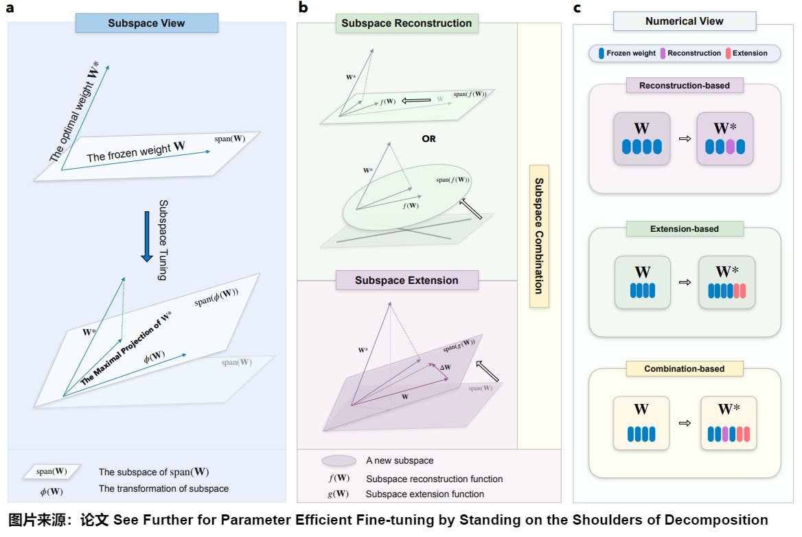
Source-local figure from A22, derived there from Si, Yang, and Shen’s decomposition framework. Retained for historical orientation. M6.7 later defines reconstruction, expansion, and composition operationally; it does not adopt the figure’s categories as a theorem.

0x00D Evidence Classes And Claim Status

This article uses five evidence classes and never treats them as interchangeable:

source-local
    what handwritten A22 says, including its organization and figure lineage

externally verified protocol or theorem
    what a pinned primary paper states under its assumptions

source-reported empirical result
    a result reported by a paper, not reproduced in this repository

executable local derivation
    algebra, finite-dimensional examples, or test oracles implemented here

rewrite interpretation
    synthesis that connects sources while preserving their scope

The source manifest pins paper revisions because theorem statements, experimental details, and even figure numbering can change between arXiv versions. A citation proves provenance; it does not by itself reproduce a training run.

0x00E Owner, Boundary, And Loop Contract

M6.7 consumes the LoRA operator, tensor shapes, first-order gradients, and checkpoint semantics from M6.3. It consumes variant axes and method-selection language from M6.4. It owns:

dimension taxonomy and intrinsic-dimension protocols
rank-manifold geometry and factor gauge
SVD reconstruction and output-weighted diagnostics
initialization asymmetry and factor dynamics
kernel-regime arguments and their failure boundary
expressive-power theorem scope
learning-versus-forgetting experimental contracts
rank-adequacy diagnostics

It explicitly defers:

variant catalog and deployment selection                 -> M6.4
adapter paging, batching, and runtime lifecycle           -> M6.5
routed, shared, and continual adapter composition         -> M6.9
general empirical scaling-law fitting and extrapolation   -> M4.7-M4.9

The article is therefore not a survey of every LoRA variant and not a claim that one theorem settles practical rank selection. Its twelve-loop reconstruction proceeds from immutable objects and protocols, through derivations and executable oracles, to paper-by-contract comparison and publication closure. Loops 1—11 now freeze the historical evidence surface, immutable study objects, intrinsic-dimension protocol, fixed-rank geometry, reconstruction and subspace diagnostics, factor dynamics, kernel and expressivity boundaries, retention decision policy, typed failures, experimental design, sources, and responsive visual provenance. Loop 12 closes formulas, browser rendering, accessibility, and cross-article ownership without changing those scientific contracts.

For provenance, the original Loop 1 entry gate is retained verbatim: “Loop 2 next freezes the parameter, matrix, function, dataset, rank, and protocol manifest.” That historical sentence records sequencing; the current handoff is Loop 12 publication closure.

0x00F Immutable Study Manifest: Objects Before Results

A low-rank result is not reproducible if its nouns can change underneath it. “The update,” “the rank,” “the dataset,” and “the baseline” are not identifiers. Two runs can use the same configured LoRA rank while adapting different tensors, starting from different base revisions, selecting checkpoints by different metrics, or measuring rank with different tolerances. They are then different experiments.

M6.7 uses one immutable study manifest with six linked namespaces:

LowRankStudyManifest(
    manifest_id       = "m6-7-linear-study-v1",

    parameter_schema  = "row-major W[4,6] -> theta[24]",
    parameter_objects = {theta_0, theta_full, delta_theta_full, u},
    matrix_objects    = {W_0, W_full, delta_W_full, A, B, delta_W_lora},
    function_objects  = {f_theta, F_train, J_train, K_train},
    dataset_objects   = {train_v1, eval_v1, retention_v1},
    rank_policies     = {configured, algebraic, numerical, stable, energy, entropy},
    protocols         = {DID, SAID, full_update, LoRA, SVD,
                         output_weighted, overlap, kernel, retention},
)

The manifest is a deliberately small linear teaching fixture. It exists so later loops can execute exact algebra and reject identity drift. It is not a miniature language model and its derived numbers are not paper results.

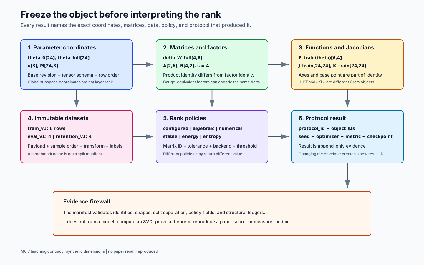
Every arrow in the figure is directional. A dataset and a parameter object determine a function trace; a measured dense update and a rank policy determine a reconstruction diagnostic; a protocol consumes those objects and emits a result record. A result record never retroactively changes the object that produced it.

0x00G Parameter Coordinates, Matrices, And Factors Have Different Identity

The teaching parameter vector has ambient dimension $D=24$ and is the row-major flattening of one matrix $W\in\mathbb{R}^{4\times6}$. The coordinate schema is part of the identity:

$$\theta_0=\operatorname{vec}_{\text{row}}(W_0) \in\mathbb{R}^{24}$$

A dense fine-tuning delta is defined only when the base and trained objects have the same tensor schema and coordinate order:

$$\Delta\theta_{full} = \theta_{full}-\theta_0, \qquad \Delta W_{full} = \operatorname{unvec}_{4\times6}(\Delta\theta_{full})$$

Changing a tensor name, transpose convention, vocabulary row order, shard layout without reconstruction, or base revision invalidates this subtraction. Shape equality alone is insufficient.

The global intrinsic-dimension fixture introduces a separate coordinate vector and a fixed projection:

$$u\in\mathbb{R}^{d}, \qquad M\in\mathbb{R}^{24\times d}, \qquad \theta(u)=\theta_0+Mu$$

The baseline manifest uses $d=3$, but this is a teaching configuration, not a measured intrinsic dimension. The protocol later sweeps candidate values of $d$ and creates a distinct projection identity for every projection family, dimension, and seed.

The LoRA fixture acts on the matrix object instead:

$$A\in\mathbb{R}^{2\times6}, \qquad B\in\mathbb{R}^{4\times2}, \qquad \Delta W_{LoRA}=sBA$$

Its configured rank is $r=2$, scale is $s=\alpha/r=4$, and factor count is $2(6+4)=20$. The factors, their product, and the dense reference update have distinct IDs. A gauge transformation can change $A$ and $B$ without changing $BA$, so a factor checkpoint cannot be compared coordinate by coordinate with another checkpoint until its gauge convention or alignment operation is declared.

Identity	Frozen fields	Legal derived object	Illegal collapse
theta_0	base revision, tensor schema, coordinate order, dtype role	function at the base point	”same shape” means same base
delta_theta_full	base ID, trained ID, subtraction schema	per-layer reshapes	a LoRA factor vector
delta_W_full	layer ID, input/output axes, base/trained IDs	SVD diagnostics	global intrinsic dimension
A, B	factor IDs, orientation, rank, scale, initialization	sBA	uniquely identifiable coordinates
delta_W_lora	factor artifact IDs and multiplication order	rank-bounded operator delta	proof that configured rank is realized
M, u	projection family, dimension, seed, ambient schema	global subspace update Mu	a layer-local low-rank factorization

0x00H Functions, Jacobians, And Datasets Are First-Class Objects

Parameter-space statements become function-space statements only after fixing inputs. For a dataset matrix $X=(x_1,\ldots,x_N)$, define the stacked output trace:

$$F_X(\theta) = \begin{bmatrix} f_{\theta}(x_1)\\ \vdots\\ f_{\theta}(x_N) \end{bmatrix}$$

If each example produces $C$ measured outputs, the dataset Jacobian at the declared base point is:

$$J_X(\theta_0) = \frac{\partial\operatorname{vec}(F_X(\theta))}{\partial\theta^{\top}} \bigg|_{\theta=\theta_0} \in\mathbb{R}^{NC\times D}$$

The corresponding empirical output-space kernel is:

$$K_X(\theta_0) = J_X(\theta_0)J_X(\theta_0)^{\top} \in\mathbb{R}^{NC\times NC}$$

$J_X^{\top}J_X\in\mathbb{R}^{D\times D}$ is a different parameter-space Gram matrix. Calling both objects “the NTK” without axes would make later kernel comparisons ambiguous.

The teaching fixture freezes three disjoint synthetic splits:

Split	Rows	Purpose	Frozen identity fields
train_v1	6	optimizer updates and train loss	ordered sample IDs, numeric payload, labels, transform revision
eval_v1	4	checkpoint selection and target score	ordered sample IDs, payload, labels, metric revision
retention_v1	4	non-target behavior	separate dataset ID, payload, labels, metric revision

Real experiments must additionally freeze model/tokenizer revision, prompt or sequence construction, truncation, label mapping, deduplication, data order, batch construction, and all random seeds. A dataset name is not a split manifest. A benchmark score without a checkpoint-selection rule is not a protocol result.

For output-weighted reconstruction, the sampled input matrix is also part of the metric:

$$E_X(r) = \left\| X\left(\Delta W_{full}-\Delta W_r\right)^{\top} \right\|_F$$

Changing $X$ changes the weighting of right-singular directions even when $\Delta W_{full}$ and $r$ are unchanged.

0x00I “Rank” Is A Policy Family, Not One Stored Integer

The manifest records the configured bottleneck and every measured-rank policy separately.

Rank record	Definition	Required policy fields	Main limitation
configured rank $r_{cfg}$	factor bottleneck chosen before training	target matrix, factor orientation, rank	only an upper bound on rank(BA)
algebraic rank $r_{alg}$	number of nonzero singular values in exact arithmetic	exact matrix object	unstable as a floating-point diagnostic
numerical rank $r_{num}$	singular values above a declared threshold	matrix, dtype, SVD backend, tolerance rule	changes with scale and tolerance
stable rank $r_{stable}$	norm-ratio proxy	matrix and norm convention	non-integer and not a factor bottleneck
energy rank $r_{\rho}$	smallest prefix capturing fraction $\rho$ of squared singular mass	matrix, sort order, energy threshold	ignores task/output weighting
entropy effective rank $r_{ent}$	exponential entropy of normalized spectral energy	matrix, zero-spectrum policy, logarithm base	another smooth summary, not algebraic rank

For the numerical-rank policy used by later teaching oracles:

$$\tau_{abs}=\tau_{rel}\sigma_1, \qquad r_{num}(\tau_{rel}) = \#\{i:\sigma_i>\tau_{abs}\}$$

The stable-rank policy is:

$$r_{stable}(\Delta W) = \frac{\|\Delta W\|_F^2}{\|\Delta W\|_2^2}$$

The energy-rank policy is:

$$r_{\rho} = \min\left\{ k: \frac{\sum_{i=1}^{k}\sigma_i^2} {\sum_j\sigma_j^2} \geq\rho \right\}$$

For entropy effective rank, let $p_i=\sigma_i^2/\sum_j\sigma_j^2$ over nonzero spectral mass:

$$r_{ent} = \exp\left(-\sum_i p_i\log p_i\right)$$

These estimators can disagree without any implementation bug because they answer different questions. Every reported rank must carry the matrix ID and policy ID that produced it.

0x00J Protocol Identity: One Result, One Envelope

The manifest gives each later experiment its own immutable envelope.

Protocol ID	Trainable object	Fixed objects	Required sweep or comparison	Result contract
did_v1	global coordinates $u$	base, projection family/seed, train/eval splits	candidate $d$ and projection seeds	score distribution and threshold-qualified $d$
said_v1	$u$ plus declared layer scales	base, structured projection, budget convention	candidate total coordinate budget	score plus explicit scale-coordinate accounting
full_update_v1	full parameter object	base and data protocol	optimizer/seed replication	checkpoint ID, score, and aligned dense delta
lora_v1	declared $A,B$ factors only	base, target matrix, scale/init	rank and seed sweep	checkpoint ID, score, and product delta
svd_reconstruction_v1	none	aligned dense delta	rank and tolerance policies	norm residuals, never task quality by itself
output_weighted_v1	none	dense delta and named input split	rank sweep	sampled output residual
subspace_overlap_v1	none	two named matrix/subspace objects	retained dimensions and normalization	principal angles or overlap statistic
kernel_v1	protocol-dependent	base point, named dataset, Jacobian convention	full versus restricted features	kernel discrepancy under declared axes
retention_v1	full or adapter parameters	matched budgets and checkpoint rule	method/rank/seed sweep	target and retention metrics together

Every training protocol records optimizer name and revision, hyperparameters, schedule, steps or tokens, batching, precision, clipping, regularization, seed roles, evaluation cadence, and checkpoint-selection rule. Every analysis protocol records the exact checkpoint IDs, matrix extraction rule, SVD/rank policy, and numerical backend. Reusing a result under a changed envelope creates a new result ID; it does not silently mutate the old one.

0x00K The Teaching Ledger And Its Evidence Boundary

The checked Loop 2 fixture derives only structural facts:

ambient parameter coordinates D                 = 24
global teaching subspace coordinates d          = 3
dense matrix coordinates 4 * 6                  = 24
configured LoRA factor coordinates 2*(6+4)      = 20
generic rank-2 matrix-manifold dimension         = 2*(6+4-2) = 16
factor gauge redundancy                         = 2^2 = 4
train / eval / retention rows                    = 6 / 4 / 4
stacked train outputs N*C                        = 6*4 = 24
train Jacobian shape                             = [24,24]
output-space empirical-kernel shape              = [24,24]

The manifest validator checks shapes, identities, split separation, rank-policy fields, protocol envelopes, and these cross-object ledgers. It does not optimize $u$, train LoRA, compute an SVD, evaluate a kernel approximation, establish an expressivity theorem, or reproduce a paper score. Those operations belong to later loops and must consume this exact manifest rather than inventing new objects mid-derivation.

0x01 A Vocabulary Of Dimensions

0x01A Ambient Parameter Dimension

Flatten every trainable model tensor into:

$$\theta\in\mathbb{R}^{D}$$

Full fine-tuning exposes up to $D$ scalar coordinates to the optimizer. $D$ is an ambient count, not proof that every coordinate is needed or independently identifiable on the downstream data.

0x01B Optimization Subspace Dimension

Choose a map $P:\mathbb{R}^{d}\rightarrow\mathbb{R}^{D}$ and optimize:

$$\theta(u)=\theta_0+P(u), \qquad u\in\mathbb{R}^{d}$$

When $P(u)=Mu$ for a fixed matrix $M\in\mathbb{R}^{D\times d}$, training is restricted to one $d$-dimensional linear subspace of the full parameter space.

This $d$ is a global optimization coordinate count. It does not describe the rank of any one reshaped parameter update.

0x01C Matrix Update Rank

For one layer:

$$\Delta W=W_{ft}-W_0 \in\mathbb{R}^{d_{out}\times d_{in}}$$

the matrix rank is the number of nonzero singular values:

$$\operatorname{rank}(\Delta W) \leq \min(d_{out},d_{in})$$

This rank says how many independent input-to-output directions the update uses at that layer. It says nothing directly about the rest of the model.

0x01D LoRA Rank

LoRA imposes:

$$\Delta W=sBA$$

and therefore:

$$\operatorname{rank}(\Delta W) \leq \min(\operatorname{rank}(A),\operatorname{rank}(B)) \leq r$$

The configured $r$ is an upper bound. Training may produce an effective update rank below $r$ because factors become dependent, singular values collapse, or regularization suppresses directions.

0x01E Representation Or Feature Dimension

Hidden states can also occupy a low-dimensional subspace on a dataset. That is an activation-space claim. A model can have low-dimensional observed features while requiring a high-rank weight update outside that sample, or a low-rank update can alter high-dimensional activations through nonlinear network composition.

0x01F Do Not Conflate The Objects

Quantity	Object	Typical measurement	What it does not prove
$D$	full parameter vector	count tensor elements	all coordinates are needed
$d_{90}$	optimization objective under a subspace protocol	repeated subspace training	one layer update has rank $d_{90}$
$\operatorname{rank}(\Delta W_l)$	one layer update	SVD with a tolerance	objective intrinsic dimension equals this rank
LoRA $r_l$	factor bottleneck	configuration	all $r_l$ directions are used
stable/effective rank	singular spectrum	threshold, entropy, or norm ratio	exact algebraic rank
feature dimension	activations/Jacobian	PCA, spectrum, kernel	parameter update is low rank

0x02 Intrinsic Dimension Is A Protocol

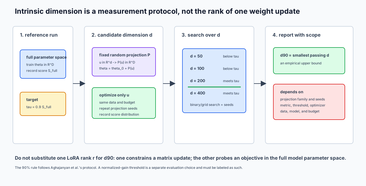
The primary intrinsic-dimension study for language-model fine-tuning defines an objective’s intrinsic dimension as the minimum number of parameters needed to reach a satisfactory solution, then estimates it through low-dimensional subspace training. The first clause is an idealized property of an objective and success criterion. The second is a finite experiment with a projection family, sampled subspaces, optimizer, budget, metric, threshold, and search grid.

The experiment can therefore return a reproducible protocol estimate. It does not reveal a unique architecture constant.

0x02A Direct Reparameterization And Gradient Pullback

Let $M\in\mathbb{R}^{D\times d}$ be a fixed random projection and $u\in\mathbb{R}^{d}$ be trainable:

$$\theta=\theta_0+Mu$$

Initialize $u=0$, so the run begins at the pretrained parameters $\theta_0$. During training:

$$\nabla_u\mathcal{L} = M^{\top}\nabla_{\theta}\mathcal{L}$$

The optimizer sees the full-model gradient only after it has been projected into $d$ coordinates. The effective full-space update is:

$$\Delta\theta = -\eta MM^{\top}\nabla_{\theta}\mathcal{L}$$

for one plain gradient-descent step. Thus the method is not selecting $d$ original parameters. It optimizes $d$ combinations of all parameters defined by $M$.

The forward and reverse tensor trace is:

forward:
    u[d]
      -> M @ u
    delta_theta[D]
      -> theta_0 + delta_theta
    theta[D]
      -> model and loss
    L[]

reverse:
    g_theta[D]
      -> M^T @ g_theta
    g_u[d]

The adjoint identity is the implementation check:

$$\langle g_{\theta},Mv\rangle = \langle M^{\top}g_{\theta},v\rangle \qquad \text{for every probe }v\in\mathbb{R}^{d}$$

It catches a wrong transpose, a changed flattening order, or a forward/adjoint projection generated from different seeds.

0x02B When $MM^{\top}$ Is And Is Not A Projector

If the columns of $M$ are orthonormal,

$$M^{\top}M=I_d$$

then:

$$\Pi_M=MM^{\top}$$

is the orthogonal projector onto $\operatorname{col}(M)$. It is symmetric and idempotent:

$$\Pi_M^{\top}=\Pi_M, \qquad \Pi_M^2=\Pi_M$$

and the rejected gradient is orthogonal to the subspace:

$$M^{\top}(I-MM^{\top})g_{\theta}=0$$

If $M$ has full column rank but non-orthonormal columns, the orthogonal projector is instead:

$$\Pi_M^{\perp} = M(M^{\top}M)^{-1}M^{\top}$$

Plain gradient descent in the coordinates $u$ still induces $-\eta MM^{\top}g_{\theta}$, not $-\eta\Pi_M^{\perp}g_{\theta}$. The reachable subspace is the same, but its coordinate metric changes the optimization trajectory. Replacing $M$ by $MR$ and $u$ by $R^{-1}u$ preserves represented points for invertible $R$, yet generally does not preserve SGD or Adam steps. A subspace identity and an optimizer-coordinate identity are separate fields.

The original objective-landscape study normalized dense random columns and relied on high-dimensional approximate orthogonality unless an explicit orthogonalization was used. A Fastfood-style map should not be called an orthogonal projector merely because it is random.

0x02C Dense, Sparse, And Implicit Projection Choices

Li et al. compared three ways to realize the fixed map. They share the same reparameterization contract but have different state and arithmetic costs.

Projection family	Stored representation	Logical application cost	Important qualification
dense Gaussian-style	$D\times d$ values	$O(Dd)$	columns can be normalized or orthogonalized; state is prohibitive at large $D$
very sparse random	nonzero values and indices	source-reported theoretical improvement over dense	sparse metadata and framework kernels determine realized cost
Fastfood-style implicit	signs, Gaussian diagonal, permutations, and block state	$O(D\log d)$ time and $O(D)$ state in the cited construction	padding, stacking, normalization, trimming, and adjoint must be implementation-defined

Aghajanyan et al. give a concrete scale example: a dense map for RoBERTa-Large with $d=1000$ would require roughly 1.42 TB for the projection alone under their accounting. That motivates an implicit map; it does not make every structured map numerically equivalent.

0x02D Fastfood Forward, Padding, Stacking, And Adjoint

Storing a dense $D\times d$ matrix is infeasible for large language models. Aghajanyan et al. use a Fastfood-style structured random transform built from Hadamard transforms, random diagonal matrices, and a permutation so the projection can be applied without materializing a dense matrix.

The paper’s schematic form is:

$$M=HG\Pi HB$$

where the factors are fixed and only $u$ is trainable. The exact normalization and dimensions belong to the implementation; the important distinction is that the measurement uses a fixed global random projection, not a learned low-rank factor at each layer.

For an executable implementation, let $p=2^{\lceil\log_2d\rceil}$, pad $u$ to $\bar u\in\mathbb{R}^{p}$, and define one normalized block:

$$y_b = \frac{1}{p} H_pG_b\Pi_bH_pB_b\bar u \in\mathbb{R}^{p}$$

The $1/p$ factor represents two $1/\sqrt p$ normalized Hadamard transforms. Other normalizations are legal only when recorded. Stack $n_b=\lceil D/p\rceil$ independently parameterized blocks and trim the last block:

$$P(u) = \operatorname{trim}_{D} \begin{bmatrix} y_1\\ \vdots\\ y_{n_b} \end{bmatrix}$$

The exact forward order is:

u[d]
  -> zero-pad to p
  -> B_b sign diagonal
  -> Hadamard
  -> Pi_b permutation
  -> G_b diagonal
  -> Hadamard
  -> divide by p
  -> stack blocks
  -> trim to D

Reverse mode must undo trimming, then apply every transpose in reverse order:

$$P_b^{\top}g_b = \frac{1}{p} B_bH_p\Pi_b^{\top}G_bH_pg_b$$

because $B_b$ and $G_b$ are diagonal and $H_p$ is symmetric. Contributions from all output blocks are summed before the padded coordinates are removed. Reusing the forward permutation instead of its inverse is a shape-correct adjoint bug.

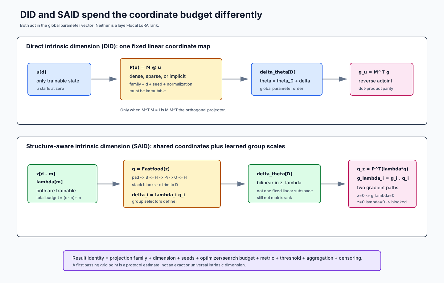
The Loop 3 exact fixture uses $D=24$, a shared coordinate width of four, six Fastfood-style blocks of width four, two parameter groups, and rational diagonal values. Rational values make the local adjoint trace exact; they are not claimed to be samples from the paper’s Gaussian distribution.

0x02E Structure-Aware Intrinsic Dimension Is Bilinear

For $m$ declared parameter groups, SAID reserves $m$ coordinates for learned group scales and uses the remaining $d-m$ coordinates for one shared projected update. Let:

$$z\in\mathbb{R}^{d-m}, \qquad q=P(z)\in\mathbb{R}^{D}$$

and let $R_i$ select the coordinates of group $i$. The update is:

$$\theta_i = \theta_{0,i}+\lambda_iR_iq$$

The total trainable-coordinate ledger is therefore:

$$d = (d-m)+m$$

not $(d-m)$ plus uncounted scale parameters. With ambient gradient $g_i=R_ig_{\theta}$, the exact gradients are:

$$\nabla_z\mathcal{L} = P^{\top} \left( \sum_{i=1}^{m}\lambda_iR_i^{\top}g_i \right)$$

and:

$$\frac{\partial\mathcal{L}}{\partial\lambda_i} = \langle g_i,R_iq\rangle$$

SAID is bilinear in $(z,\lambda)$. If $z=0$ but $\lambda_i\neq0$, scale gradients begin at zero while $z$ can receive a gradient. If both $z=0$ and every $\lambda_i=0$, both paths are blocked. Initialization is therefore part of the protocol, not harmless metadata.

The case $d=m$ has no shared projected coordinate. It is a legal coordinate count but a degenerate no-update fixture when $z$ is empty. A search implementation must report that outcome rather than silently reinterpret $d$ as the shared width.

SAID is still not LoRA. Its learned scales multiply groups of one global projected update; it does not constrain each reshaped matrix to a product of rank at most $r$.

0x02F The $d_{90}$ Grid Estimate

The protocol first obtains a full-fine-tuning score $S_{full}$, then searches for the smallest $d$ whose subspace-trained score reaches a specified fraction, historically 90%:

$$\widehat d_{90}^{\mathcal G} = \min\left\{ d\in\mathcal G: \mathcal A_{s}\left[ \max_{h\in\mathcal H}S(d,s,h) \right] \geq0.9S_{full} \right\}$$

Here $\mathcal G$ is the candidate-dimension grid, $s$ indexes projection/training seeds, $h$ indexes the declared hyperparameter search, and $\mathcal A_s$ is a declared seed aggregator such as the median. The superscript $\mathcal G$ matters: the result is the first passing tested value, not the exact minimum over all integers or all possible subspaces.

If accuracy is 85%, the historical threshold example is $0.9\times85\%=76.5\%$. This multiplication only makes sense for a score whose scale and direction support it. Loss, perplexity, signed correlation, or offset metrics need a quality transform and threshold defined in that metric’s own contract.

That threshold has a limitation: it ignores the pretrained baseline. If the base model already scores 75%, reaching 76.5% captures only a small fraction of the full fine-tuning gain. A deployment audit may instead use normalized gain:

$$G_d = \frac{S_d-S_{base}}{S_{full}-S_{base}}$$

and require $G_d\geq\tau$. This is an evaluation alternative, not the original paper’s $d_{90}$ definition.

The Loop 3 synthetic result table uses:

base score                                  0.600
full-reference score                        0.850
historical 0.9 * full threshold             0.765
90% normalized-gain threshold               0.825

DID median score at d = 4 / 6 / 8           0.750 / 0.780 / 0.830
SAID median score at d = 2 / 4 / 6 / 8      0.600 / 0.770 / 0.810 / 0.840

Under the historical threshold, the grid estimates are DID $\widehat d_{90}^{\mathcal G}=6$ and SAID $\widehat d_{90}^{\mathcal G}=4$. Under the normalized-gain threshold, both first pass at $d=8$. These are deliberately synthetic scores used to test selection semantics. They are not Aghajanyan et al.’s measurements.

0x02G Crossing, Bracketing, Censoring, And Non-Monotonicity

A result record has three possible boundary states:

crossed within grid:
    first passing tested d and previous tested d form a grid bracket

first tested d already passes:
    left-censored; report d_estimate <= d_min, not d_estimate = d_min

no tested d passes:
    right-censored or optimization-unreached; report > d_max / unresolved,
    not d_estimate = d_max

Random-subspace scores need not be monotone in $d$ across independently sampled projections. A larger candidate can receive an unlucky subspace, optimizer path, or hyperparameter choice. Do not force scores through a cumulative maximum before publishing them. Define the selection rule, preserve raw results, and report uncertainty across seeds.

For the synthetic DID table, $d=4$ fails and $d=6$ passes, so the tested-grid bracket is $(4,6]$. This is not proof that every integer between four and six behaves monotonically.

0x02H What The Primary Protocol Actually Ran

The pinned language-model study reports, for its sentence-prediction experiments:

dimensions d from 10 to 10,000 on a log scale
100 subspace-training runs per dataset/model sweep
a small search across four learning rates per training run
u initialized to zero so the base pretrained point is preserved
the randomly initialized classification head included in the d-coordinate budget
both DID and SAID implemented through a Fastfood-style transform

For its pretraining-trajectory experiment, it instead reports a binary search from 100 to four million and reuses learning rates under a stated rule. These are source-reported protocol details. They should not be blended into one fictional universal search.

The earlier objective-landscape paper used multiple projection constructions and, in several plots, defined crossing from the median of three runs. Its appendix explicitly treats the estimated intrinsic dimension as projection- and experiment-dependent. M6.7 preserves that caution rather than copying only a headline number.

0x02I Executable Direct And SAID Oracles

Loop 3 checks three independent mechanisms:

1. a $D=24,d=3$ exact orthonormal teaching matrix verifies $M^{\top}M=I$, gradient pullback, projector idempotence, rejected-gradient orthogonality, and adjoint parity;
2. a six-block, width-four Fastfood-style rational trace verifies padding, block order, stacking, trimming, inverse permutation, transpose accumulation, and adjoint parity;
3. a two-group SAID trace verifies the coordinate ledger, $z$ and $\lambda$ gradients, the first- and second-order coefficients of its bilinear directional polynomial, and initialization blocking.

For a linear probe loss $\mathcal L=g^{\top}\Delta\theta$, perturbing both SAID coordinate classes gives:

$$\mathcal L(z+t\dot z,\lambda+t\dot\lambda) = \mathcal L(z,\lambda) +t\left( \langle\nabla_z\mathcal L,\dot z\rangle +\langle\nabla_{\lambda}\mathcal L,\dot\lambda\rangle \right) +t^2\sum_i\dot\lambda_i \langle g_i,R_iP(\dot z)\rangle$$

The nonzero quadratic coefficient is direct evidence that learned group scales make the coordinate map bilinear rather than one fixed linear subspace.

0x02J Measurement Pseudocode

def estimate_intrinsic_dimension(
    pretrained,
    train_data,
    eval_data,
    candidate_dims,
    projection_seeds,
    hyperparameter_candidates,
    seed_aggregate=median,
    threshold_ratio=0.90,
):
    full_score = train_and_evaluate(
        model=clone(pretrained),
        trainable="all_parameters",
        train_data=train_data,
        eval_data=eval_data,
    )
    target = threshold_ratio * full_score

    records = []  # append-only run records; never overwrite failed seeds
    for d in candidate_dims:
        selected_seed_scores = []
        for seed in projection_seeds:
            projection = fixed_structured_projection(
                ambient_dim=pretrained.num_parameters(),
                subspace_dim=d,
                seed=seed,
            )
            trials = []
            for hyperparameters in hyperparameter_candidates:
                u = zeros(d, requires_grad=True)
                result = train_subspace_coordinates(
                    pretrained=pretrained,
                    coordinates=u,
                    projection=projection,
                    train_data=train_data,
                    eval_data=eval_data,
                    hyperparameters=hyperparameters,
                )
                trials.append(result)

            selected = select_by_declared_eval_rule(trials)
            selected_seed_scores.append(selected.score)
            records.extend(trials)

        aggregate = seed_aggregate(selected_seed_scores)
        append_dimension_summary(d, aggregate, selected_seed_scores)

    return classify_grid_crossing(
        raw_records=records,
        target=target,
        preserve_censoring=True,
    )

For SAID, subspace_dim=d must be replaced by shared_dim=d-m, and the manifest must count the $m$ learned scales inside the same total budget. A classification head, prompt parameters, or other trainable branch must likewise be included or separately disclosed.

0x02K What The Result Does And Does Not Mean

The experiment supplies an empirical upper-bound estimate under the sampled subspaces and training procedure. Failure at dimension $d$ does not prove that no useful $d$-dimensional subspace exists; the sampled map, coordinate metric, optimizer, budget, or hyperparameter search may have failed. A seed aggregate passing does show that the declared protocol reached its threshold at a tested coordinate budget.

It still does not establish:

that every random subspace of dimension d succeeds
that the exact minimum lies at the first passing grid value
that another projection family has the same coordinate geometry
that a per-layer update has matrix rank d
that a LoRA adapter with rank d is equivalent
that lower protocol dimension causes better generalization
that source-reported model-size trends extrapolate universally

Publish the raw run table, projection and seed identities, optimizer/search budget, metric direction, full and base references, threshold definition, aggregation rule, and censoring state. Without that envelope, $d_{90}$ is a slogan rather than a measurement.

0x03 The Geometry Of One LoRA Update

Loop 3 measured a global optimization-coordinate protocol. This section changes objects. It studies one matrix:

$$\Delta W\in\mathbb{R}^{m\times n}, \qquad m=d_{out},\quad n=d_{in}$$

represented by:

$$\phi(B,A)=BA, \qquad B\in\mathbb{R}^{m\times r}, \quad A\in\mathbb{R}^{r\times n}$$

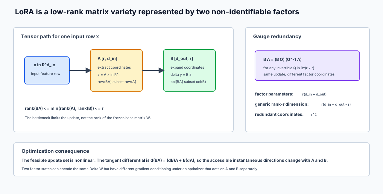
The owner question is: how many locally distinct matrix directions does this factorization represent, and which factor-coordinate changes leave the matrix unchanged?

0x03A Row Space, Column Space, And Rank Bound

Every output column of $BA$ is a linear combination of the columns of $B$:

$$\operatorname{col}(BA)\subseteq\operatorname{col}(B)$$

Likewise, every row is a linear combination of the rows of $A$:

$$\operatorname{row}(BA)\subseteq\operatorname{row}(A)$$

Therefore:

$$\operatorname{rank}(BA) \leq \min\{\operatorname{rank}(B),\operatorname{rank}(A)\} \leq r$$

Applied to one input $x\in\mathbb{R}^{n}$:

$$x\xrightarrow{A}z=Ax\in\mathbb{R}^{r} \xrightarrow{B}\Delta y=Bz\in\mathbb{R}^{m}$$

$A$ extracts $r$ latent input coordinates. $B$ maps those coordinates into output directions. The factor-role interpretation is useful, but the letters are not universal across papers or codebases. M6.3 remains authoritative for the repository’s operator orientation.

0x03B Exact Rank, Rank At Most, And The Strata Boundary

Three sets must remain separate:

$$\mathcal{R}_{=r} = \{W\in\mathbb{R}^{m\times n}:\operatorname{rank}(W)=r\}$$ $$\mathcal{R}_{\leq r} = \{W\in\mathbb{R}^{m\times n}:\operatorname{rank}(W)\leq r\}$$

and the factor-coordinate space:

$$\mathcal{F}_{r} = \mathbb{R}^{m\times r}\times\mathbb{R}^{r\times n}$$

Vandereycken proves that $\mathcal{R}_{=r}$ is a smooth embedded manifold. The closure $\mathcal{R}_{\leq r}$ also contains lower-rank strata. Those lower-rank points are singular for the rank-at-most-$r$ variety: one cannot attach the same rank-$r$ tangent dimension to every factor product.

Standard LoRA parameterization maps all of $\mathcal F_r$ into $\mathcal R_{\leq r}$. It does not guarantee that $A$, $B$, or $BA$ realize rank $r$ during training.

0x03C Derivation One: Choose Two Subspaces And An Invertible Core

At a generic exact-rank point, write a compact SVD:

$$W=U\Sigma V^{\top}, \qquad U\in\mathbb{R}^{m\times r}, \quad V\in\mathbb{R}^{n\times r}, \quad \sigma_r>0$$

The column space is a point in the Grassmannian $\operatorname{Gr}(r,m)$, whose dimension is:

$$\dim\operatorname{Gr}(r,m)=r(m-r)$$

The row space contributes:

$$\dim\operatorname{Gr}(r,n)=r(n-r)$$

Once the two subspaces are fixed, the map between them is an invertible $r\times r$ core with $r^2$ coordinates. Hence:

$$\begin{aligned} \dim\mathcal R_{=r} &=r(m-r)+r(n-r)+r^2\\ &=r(m+n-r) \end{aligned}$$

This derivation counts represented matrices directly. It does not begin from LoRA factors.

0x03D Derivation Two: Factor Coordinates Minus The $GL(r)$ Fibre

The factors store:

$$P_{factor}=mr+rn=r(m+n)$$

coordinates. For every invertible $Q\in GL(r)$:

$$(BQ)(Q^{-1}A)=BA$$

so an entire $r^2$-dimensional change of latent basis represents the same matrix. Billaud-Friess et al. formalize this fixed-rank geometry through a principal bundle whose typical fibre is $GL(r)$.

Subtracting the fibre dimension gives the same count:

$$r(m+n)-r^2 = r(m+n-r)$$

This is not a claim that $r^2$ factor entries are individually unused. The redundancy is a coupled transformation of both factors.

A concrete shear makes the equivalence visible:

$$Q= \begin{bmatrix} 1&1\\ 0&1 \end{bmatrix}, \qquad Q^{-1}= \begin{bmatrix} 1&-1\\ 0&1 \end{bmatrix}$$

$B$ and $A$ change, their norms and conditioning can change, but their product does not.

0x03E The Factor Map Differential And Its Adjoint

Perturb both factors:

$$(B+t\dot B)(A+t\dot A) = BA +t(\dot BA+B\dot A) +t^2\dot B\dot A$$

The first-order factor-to-matrix map is therefore:

$$D\phi_{B,A}(\dot B,\dot A) = \dot BA+B\dot A$$

The quadratic remainder is why the full feasible set is not one linear subspace. The tangent image is linear only after the base factors $(B,A)$ are fixed.

For an ambient probe $G\in\mathbb{R}^{m\times n}$, Frobenius adjointness gives:

$$\left\langle G,D\phi_{B,A}(\dot B,\dot A)\right\rangle_F = \left\langle GA^{\top},\dot B\right\rangle_F + \left\langle B^{\top}G,\dot A\right\rangle_F$$

Thus:

$$D\phi_{B,A}^{*}(G) = \left(GA^{\top},B^{\top}G\right)$$

This is a geometry identity and an executable transpose check. M6.3 owns the complete LoRA backward operator, dropout, scale, and base-weight integration. Loop 7 will own optimizer dynamics and conditioning.

The tensor and flattening contract used by the Loop 4 oracle is:

factor perturbation vector[20]:
    vec_row_major(dot_B[4,2])
    then vec_row_major(dot_A[2,6])

Dphi Jacobian J_phi[24,20]:
    one output column per factor-coordinate basis vector
    each output column = vec_row_major(dot_B A + B dot_A)

ambient matrix vector[24]:
    vec_row_major(dot_W[4,6])

Changing any one of those orders changes the Jacobian even though every shape still fits.

0x03F The Infinitesimal Gauge Is The Differential Kernel

Let $Q(t)=I+tK+O(t^2)$ for arbitrary $K\in\mathbb{R}^{r\times r}$. Then:

$$BQ(t)=B+tBK+O(t^2)$$

and:

$$Q(t)^{-1}A=A-tKA+O(t^2)$$

The associated factor perturbation is:

$$(\dot B,\dot A)=(BK,-KA)$$

Applying the differential:

$$D\phi_{B,A}(BK,-KA) = BKA-BKA =0$$

When $B$ has full column rank and $A$ has full row rank, these $r^2$ independent gauge directions span the entire kernel of $D\phi$. Rank-nullity then gives:

$$\operatorname{rank}(D\phi) = r(m+n)-r^2 = r(m+n-r)$$

This proves the same dimension a third way: by the rank of the local factor-to-matrix Jacobian.

0x03G Tangent Space From The Compact SVD

For $W=U\Sigma V^{\top}\in\mathcal R_{=r}$, Vandereycken gives:

$$T_W\mathcal R_{=r} = \left\{ UMV^{\top}+U_pV^{\top}+UV_p^{\top} \right\}$$

with:

$$M\in\mathbb{R}^{r\times r}, \qquad U^{\top}U_p=0, \qquad V^{\top}V_p=0$$

The three blocks have dimensions:

$$r^2, \qquad (m-r)r, \qquad (n-r)r$$

and sum to $r(m+n-r)$. The first block changes the core inside the current row/column spaces. The second rotates the column space. The third rotates the row space.

For full-rank factors with $W=BA$, the same tangent space is the image:

$$T_W\mathcal R_{=r} = \operatorname{im}D\phi_{B,A} = \{\dot BA+B\dot A\}$$

The factor differential and SVD chart are two coordinate descriptions of the same local matrix directions.

0x03H Normal Space And Orthogonal Tangent Projector

Define the orthogonal subspace projectors:

$$P_U=UU^{\top}, \qquad P_V=VV^{\top}$$

For any ambient matrix $Z$, the Frobenius-orthogonal tangent projection is:

$$\mathcal P_T(Z) = P_UZ+ZP_V-P_UZP_V$$

The equivalent normal component is:

$$\mathcal P_N(Z) = (I-P_U)Z(I-P_V)$$

Expanding the normal expression proves the decomposition:

$$Z=\mathcal P_T(Z)+\mathcal P_N(Z)$$

The normal space can also be recognized without an SVD. A matrix $N$ is orthogonal to every $\dot BA+B\dot A$ exactly when:

$$B^{\top}N=0, \qquad NA^{\top}=0$$

Its dimension is:

$$(m-r)(n-r)$$

so ambient dimension reconciles:

$$mn = r(m+n-r) + (m-r)(n-r)$$

Do not confuse $\mathcal P_T(G)$ with one Euclidean SGD step in arbitrary factors. The former is the orthogonal matrix-space projection. The latter depends on the chosen factor gauge and optimizer metric.

0x03I Exact $4\times6$, Rank-Two Reconciliation

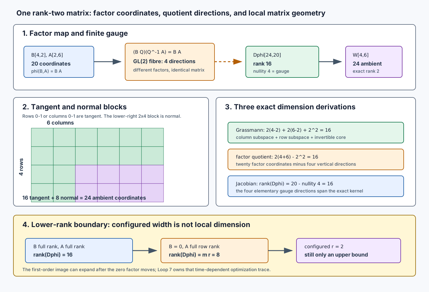
The Loop 2 matrix schema fixes:

m = 4 output rows
n = 6 input columns
r = 2 configured factor width
ambient matrix coordinates             = 4*6                 = 24
factor coordinates                     = 4*2 + 2*6           = 20
finite/infinitesimal GL(2) gauge       = 2*2                 = 4
generic exact-rank-2 manifold          = 2*(4+6-2)           = 16
normal-space coordinates               = (4-2)*(6-2)         = 8
tangent + normal                       = 16 + 8               = 24
factor - gauge                         = 20 - 4               = 16

The exact fixture chooses:

$$B= \begin{bmatrix} 1&0\\ 0&1\\ 0&0\\ 0&0 \end{bmatrix}, \qquad A= \begin{bmatrix} 1&0&0&0&0&0\\ 0&1&0&0&0&0 \end{bmatrix}$$

so $W=BA$ has rank two. The factor Jacobian has shape $24\times20$, exact rank 16, and nullity four. Four gauge basis vectors generated by the elementary $2\times2$ matrices lie in its kernel and have rank four, so they span that kernel.

For an ambient probe containing row-major values 1 through 24, $\mathcal P_T$ retains the first two rows and the first two columns of the last two rows. $\mathcal P_N$ retains only the lower-right $2\times4$ block. The oracle verifies:

P_T + P_N equals the original probe
P_T and P_N are Frobenius orthogonal
P_T is symmetric and idempotent as a 24x24 operator
Dphi* satisfies exact dot-product parity
every normal probe satisfies B^T N = 0 and N A^T = 0

0x03J What Breaks At A Lower-Rank Factor Point

Now keep $A$ full row rank but set $B=0$. The represented matrix is rank zero, not rank two. The differential becomes:

$$D\phi_{0,A}(\dot B,\dot A) = \dot BA$$

All $\dot A$ directions disappear at first order. For the $4\times6,r=2$ fixture, the differential rank drops from 16 to:

$$mr=8$$

This is the exact local geometry behind the familiar first-step asymmetry of a zero-product initialization. It does not mean training is permanently confined to eight dimensions: once $B$ moves, the $B\dot A$ path can open. Loop 7 derives that time-dependent optimization behavior.

The key distinction is:

configured factor width r:
    storage and rank upper bound

realized product rank:
    rank of BA at one checkpoint

factor-Jacobian rank:
    number of first-order matrix directions available at (B,A)

rank-r manifold dimension:
    generic local dimension only when the represented matrix has exact rank r

0x03K Coordinate Choices And Design Alternatives

Representation	Coordinates	Redundancy or constraint	Local implication
unconstrained factors $BA$	$r(m+n)$	$GL(r)$ gauge	simple dense factors; Euclidean optimizer is gauge-dependent
compact SVD $U\Sigma V^{\top}$	nominally $r(m+n+1)$ entries	Stiefel constraints plus sign/rotation conventions	exposes row, column, and core geometry; updates require constraint handling
quotient-manifold factors	$r(m+n-r)$ effective	gauge classes are identified by the metric/connection	removes vertical directions conceptually; needs specialized optimization
fixed $A$, train $B$	$mr$	row subspace fixed by $A$	first-order image is at most $mr$ and cannot rotate the row basis through $A$
fixed $B$, train $A$	$rn$	column subspace fixed by $B$	first-order image is at most $rn$
fixed row and column bases, train core	$r^2$	both subspaces fixed	changes only the map inside existing subspaces
dense update	$mn$	no rank restriction	maximal local freedom and full training state

This table compares geometry, not benchmark quality. M6.4 owns adaptation-method selection and composition. M6.7 only states what each coordinate choice can represent locally.

0x03L Executable Geometry Oracle

def factor_map_jacobian(B, A):
    columns = []

    # Row-major B coordinates first.
    for i in range(B.rows):
        for j in range(B.cols):
            dot_B = basis_matrix(B.shape, i, j)
            columns.append(row_major_flatten(dot_B @ A))

    # Then row-major A coordinates.
    for i in range(A.rows):
        for j in range(A.cols):
            dot_A = basis_matrix(A.shape, i, j)
            columns.append(row_major_flatten(B @ dot_A))

    return stack_columns(columns)  # [m*n, m*r+r*n]


def tangent_project(Z, U, V):
    P_U = U @ U.T
    P_V = V @ V.T
    return P_U @ Z + Z @ P_V - P_U @ Z @ P_V


def normal_project(Z, U, V):
    return (I_m - U @ U.T) @ Z @ (I_n - V @ V.T)

The checked $m=4,n=6,r=2$ oracle uses exact rational elimination rather than a floating-point rank tolerance. It obtains a $24\times20$ factor Jacobian of rank $16$, a four-dimensional nullspace spanned by the four elementary gauge directions, a rank-$16$ tangent projector, and a rank-$8$ normal projector. At the lower-rank fixture $B=0$ with full-row-rank $A$, the same coordinate map has differential rank $8$ and nullity $12$. All 58 one-field counterexamples are rejected. Later empirical rank diagnostics must name their numerical threshold separately.

0x03M Per-Layer Restrictions Compose Through A Nonlinear Network

If every adapted matrix has rank at most $r$, the end-to-end function change need not have rank $r$ in any simple global sense. Residual connections, nonlinearities, attention, and layer composition combine local matrix changes.

Conversely, a desired end-to-end behavior may require several layers to change jointly even if each local update is low rank. Adapting more projection types at modest rank can therefore outperform placing a larger rank on one matrix in a specific experiment. That observation is source-reported evidence, not a theorem obtained from the manifold dimension.

0x04 Reconstruction: What Rank $r$ Can Approximate

0x04A Freeze The Object Before Decomposing It

The reconstruction target is not an unnamed “fine-tuning direction.” It is the immutable Loop 2 object:

$$\Delta W^*=W_{full}-W_0\in\mathbb{R}^{m\times n}, \qquad (m,n)=(4,6)$$

with object ID matrix_delta:W_full-minus-W_0:layer0.linear:v1, output-by-input orientation, and one fixed checkpoint-selection contract. Changing the base revision, adapted tensor, subtraction order, or checkpoint creates a different matrix and invalidates the comparison.

For $q=\min(m,n)$, its compact singular value decomposition is:

$$\Delta W^*=U\Sigma V^{\top}, \qquad U\in\mathbb{R}^{m\times q}, \quad \Sigma\in\mathbb{R}^{q\times q}, \quad V^{\top}\in\mathbb{R}^{q\times n}$$

where $U^{\top}U=I_q$, $V^{\top}V=I_q$, and:

$$\Sigma=\operatorname{diag}(\sigma_1,\ldots,\sigma_q), \qquad \sigma_1\geq\cdots\geq\sigma_q\geq0$$

The full SVD may add orthonormal columns spanning unused complements. Those extra columns do not change the nonzero singular expansion. Compact and full SVD are storage choices, not different reconstructions.

0x04B Why Truncation Solves The Frobenius Problem

The singular expansion is a sum of Frobenius-orthogonal rank-one atoms:

$$\Delta W^*=\sum_{i=1}^{q}\sigma_i u_i v_i^{\top}, \qquad \left\langle u_i v_i^{\top},u_j v_j^{\top}\right\rangle_F=\delta_{ij}$$

Keeping the first $r$ atoms gives:

$$\Delta W_r^*=U_r\Sigma_rV_r^{\top} =\sum_{i=1}^{r}\sigma_i u_i v_i^{\top}$$

and orthogonality immediately gives its tail error:

$$\left\|\Delta W^*-\Delta W_r^*\right\|_F^2 =\left\|\sum_{i>r}\sigma_i u_i v_i^{\top}\right\|_F^2 =\sum_{i>r}\sigma_i^2$$

That calculation proves the residual of truncation, but optimality requires a lower bound for every other rank-at-most-$r$ matrix $R$. Let $P$ project onto any $(n-r)$-dimensional subspace of $\ker(R)$. Then $RP=0$, so:

$$\begin{aligned} \|\Delta W^*-R\|_F^2 &\geq \|(\Delta W^*-R)P\|_F^2 \\ &=\|\Delta W^*P\|_F^2 \\ &=\operatorname{tr}\left(P(\Delta W^*)^{\top}\Delta W^*P\right) \end{aligned}$$

The Rayleigh—Ritz minimum over all such projectors selects the right-singular directions with the $n-r$ smallest eigenvalues of $(\Delta W^*)^{\top}\Delta W^*$. Its value is $\sum_{i>r}\sigma_i^2$. Truncation reaches that lower bound, which is the Eckart—Young least-squares result.

The spectral-norm lower bound has an equally useful geometric proof. The $(r+1)$-dimensional space $S=\operatorname{span}(v_1,\ldots,v_{r+1})$ must intersect $\ker(R)$ in a nonzero vector. For a unit $x$ in that intersection:

$$\|\Delta W^*-R\|_2 \geq\|(\Delta W^*-R)x\|_2 =\|\Delta W^*x\|_2 \geq\sigma_{r+1}$$

and $\Delta W_r^*$ reaches the bound:

$$\|\Delta W^*-\Delta W_r^*\|_2=\sigma_{r+1}$$

For the Frobenius objective, a strict gap $\sigma_r>\sigma_{r+1}$ makes the rank-$r$ truncated matrix unique. A tie at the boundary permits several optimal $r$-dimensional singular subspaces. “The SVD” therefore does not always identify one unique factor pair, and the $GL(r)$ gauge from 0x03 means even a unique reconstructed matrix has many factorizations.

0x04C Matrix Reconstruction And LoRA Optimization Are Different Experiments

One exact factorization of the truncation is:

$$B_r=U_r\Sigma_r\in\mathbb{R}^{m\times r}, \qquad A_r=V_r^{\top}\in\mathbb{R}^{r\times n}, \qquad B_rA_r=\Delta W_r^*$$

A balanced choice can split $\Sigma_r^{1/2}$ across both factors. The two choices are gauge-equivalent matrix representations when all retained singular values are nonzero. Neither is the trajectory produced automatically by stochastic LoRA training.

post-hoc truncated SVD
    input: one already-measured dense update
    operation: deterministic matrix decomposition
    objective: best matrix residual under a named norm

LoRA optimization
    input: base model, factors, data, optimizer, and initialization
    operation: bilinear training through the model loss
    objective: training objective under a finite budget

SVD answers whether a dense reference is compressible after the fact. It does not prove that rank-$r$ LoRA reaches the same matrix, the same function, or the same task quality.

0x04D Exact $4\times6$ Rank Sweep

The executable fixture uses:

$$\Delta W^*= \begin{bmatrix} 4&0&0&0&0&0\\ 0&3&0&0&0&0\\ 0&0&2&0&0&0\\ 0&0&0&1&0&0 \end{bmatrix}, \qquad \sigma=(4,3,2,1)$$

Therefore $\|\Delta W^*\|_F^2=16+9+4+1=30$. Every row below is reconstructed from the declared $B_rA_r$ factors using exact rational arithmetic:

$r$	retained squared energy	retained singular-value mass	$\|\Delta W^*-\Delta W_r^*\|_F^2$	$\|\Delta W^*-\Delta W_r^*\|_2$
0	$0$	$0$	$30$	$4$
1	$8/15$	$2/5$	$14$	$3$
2	$5/6$	$7/10$	$5$	$2$
3	$29/30$	$9/10$	$1$	$1$
4	$1$	$1$	$0$	$0$

The second and third columns are deliberately both present. “Retains 90% of the singular values” is ambiguous: sum of singular values and sum of squared singular values are different mass policies.

0x04E Derive Sampled Output Error From Tensor Shapes

Weight-space Frobenius error weights every matrix entry equally. A linear layer sees inputs. Let:

$$X\in\mathbb{R}^{N\times n}, \qquad \widehat{\Delta W}\in\mathbb{R}^{m\times n}, \qquad R=\Delta W^*-\widehat{\Delta W}\in\mathbb{R}^{m\times n}$$

The changed layer outputs are $X(\Delta W^*)^{\top}$ and $X\widehat{\Delta W}^{\top}$, both in $\mathbb{R}^{N\times m}$. Their mean squared residual is:

$$\mathcal{L}_X(\widehat{\Delta W}) =\frac{1}{N}\|XR^{\top}\|_F^2$$

Move through the trace one operation at a time:

$$\begin{aligned} \frac{1}{N}\|XR^{\top}\|_F^2 &=\frac{1}{N}\operatorname{tr}(XR^{\top}RX^{\top}) \\ &=\operatorname{tr}\left(R\frac{X^{\top}X}{N}R^{\top}\right) \\ &=\operatorname{tr}(RC_XR^{\top}) \end{aligned}$$

where:

$$C_X=\frac{1}{N}X^{\top}X\in\mathbb{R}^{n\times n}$$

Because $C_X$ is positive semidefinite, it has a positive-semidefinite square root. The same objective is:

$$\mathcal{L}_X(\widehat{\Delta W}) =\|RC_X^{1/2}\|_F^2 =\|\Delta W^*C_X^{1/2}-\widehat{\Delta W}C_X^{1/2}\|_F^2$$

This derivation explains the final form: calibration variance stretches input directions before reconstruction error is measured.

0x04F Full-Rank Covariance Turns The Problem Into A Whitened SVD

If $C_X\succ0$, multiplication by $C_X^{1/2}$ is invertible and preserves rank. Define:

$$M=\Delta W^*C_X^{1/2}, \qquad Z=\widehat{\Delta W}C_X^{1/2}$$

Then $\operatorname{rank}(Z)=\operatorname{rank}(\widehat{\Delta W})$, so:

$$\min_{\operatorname{rank}(\widehat{\Delta W})\leq r} \mathcal{L}_X(\widehat{\Delta W}) = \min_{\operatorname{rank}(Z)\leq r}\|M-Z\|_F^2$$

Eckart—Young now applies to $M$, not generally to $\Delta W^*$:

$$Z^*=M_r, \qquad \widehat{\Delta W}_{X,r}=M_rC_X^{-1/2}$$

The matrix to decompose is $\Delta W^*C_X^{1/2}$. Replacing the square root by $C_X$ changes the objective. CorDA is a useful context-oriented design alternative, but its decomposition of pretrained $WC_X$ and inverse-covariance reconstruction belong to CorDA’s method contract; they are not this output-error theorem.

0x04G Singular Covariance Exposes A Calibration Blind Spot

Real activation covariances can be singular because $N<n$, features are dependent, or some directions are absent. Let:

$$C_X=Q_+\Lambda_+Q_+^{\top}, \qquad \Lambda_+\succ0$$

on the observed support. A minimum-norm optimal representative is:

$$\widehat{\Delta W}_{X,r} =(\Delta W^*C_X^{1/2})_rC_X^{\dagger/2}$$

where $\dagger$ denotes the Moore—Penrose pseudoinverse. But any matrix $N_0$ satisfying $N_0C_X^{1/2}=0$ is invisible to the sampled loss:

$$\mathcal{L}_X(\widehat{\Delta W}+N_0) =\mathcal{L}_X(\widehat{\Delta W})$$

Such additions can change matrix rank and behavior outside the calibration support. The sampled objective therefore does not identify a unique global update. It identifies behavior only on directions represented by $X$.

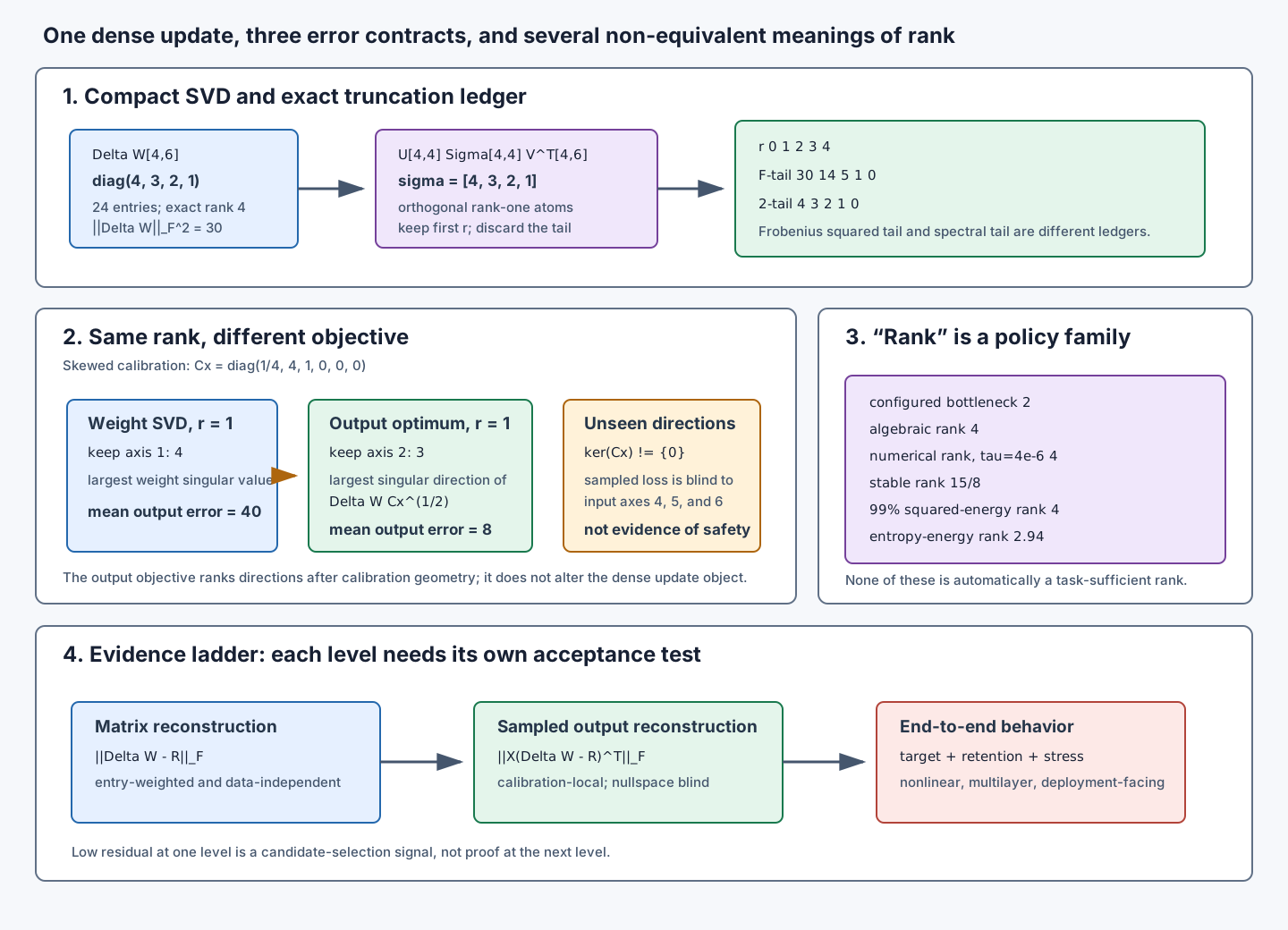
0x04H Same Rank, Different Winner: An Exact Counterexample

The immutable train_v1 split is the six-dimensional identity basis. It gives $C_X=I_6/6$, so its raw output residual equals the Frobenius residual and its mean output residual is one sixth of that value. This validates tensor orientation, but it cannot expose a difference in direction weighting.

Loop 5 therefore adds a separately named sensitivity probe, without replacing train_v1:

$$X_{skew}= \begin{bmatrix} 1&0&0&0&0&0\\ 0&4&0&0&0&0\\ 0&0&2&0&0&0\\ 0&0&0&0&0&0 \end{bmatrix}, \qquad C_{skew}=\operatorname{diag}\left(\frac14,4,1,0,0,0\right)$$

The ordinary weight-space rank-one truncation keeps the first axis because $4>3$. The transformed update is:

$$\Delta W^*C_{skew}^{1/2}=\operatorname{diag}(2,6,2,0)$$

so the output-weighted rank-one solution keeps the second axis. Exact direct multiplication and the covariance trace agree:

rank-constrained candidate	retained update axis	raw $\|X_{skew}R^{\top}\|_F^2$	mean output residual
weight-SVD rank one	axis 1, value $4$	$160$	$40$
output-optimal rank one	axis 2, value $3$	$32$	$8$
weight-SVD rank two	axes 1 and 2	$16$	$4$

The output optimum is five times better than the weight optimum at the same rank. Yet the zero covariance on input axes 4—6 means this probe assigns zero loss to some nonzero residuals. Better calibration fit is not a task-safety guarantee.

0x04I Rank Is A Family Of Named Policies

For the same fixed matrix with spectrum $(4,3,2,1)$, the immutable policies report:

policy	definition	result	what it answers
configured LoRA rank	factor bottleneck width	$2$	maximum rank the configured factors can express
algebraic rank	exact count of nonzero singular values	$4$	exact matrix rank
numerical rank	count $\sigma_i>10^{-6}\sigma_1$	$4$	rank under one relative tolerance
stable rank	$\|\Delta W^*\|_F^2/\|\Delta W^*\|_2^2$	$30/16=15/8$	continuous spectral concentration
99% energy rank	smallest $r$ with squared-energy prefix at least $0.99$	$4$	budget for one named energy threshold
entropy-energy rank	$\exp[-\sum_i p_i\ln p_i]$, $p_i=\sigma_i^2/\sum_j\sigma_j^2$	$2.9402$	continuous effective count under squared energy
task-sufficient rank	smallest rank passing target, retention, and stress gates	not measured here	deployment adequacy under one protocol

Numerical rank depends on scale and tolerance. The threshold probe uses singular values $(4,1,1/250000,0)$ with $\tau=10^{-6}\sigma_1=1/250000$. Because the frozen policy is strictly greater than, the boundary value is excluded and the numerical rank is two. A >= implementation would silently return three.

0x04J Two Entropy Conventions Must Not Share One Label

Roy and Vetterli’s effective rank normalizes singular values:

$$p_i^{RV}=\frac{\sigma_i}{\sum_j\sigma_j}, \qquad r_{eff}^{RV}=\exp\left(-\sum_i p_i^{RV}\ln p_i^{RV}\right)$$

For $(4,3,2,1)$ this gives $r_{eff}^{RV}\approx3.5961$. The Loop 2 manifest deliberately defines a different entropy-energy diagnostic:

$$p_i^{E}=\frac{\sigma_i^2}{\sum_j\sigma_j^2}, \qquad r_{eff}^{E}=\exp\left(-\sum_i p_i^{E}\ln p_i^{E}\right) \approx2.9402$$

Both are valid continuous summaries when named. They are not the same statistic. For the zero matrix the normalization has zero mass, so the manifest explicitly returns effective rank zero instead of dividing by zero or inventing a probability distribution.

0x04K Tensor And Code Trace

def reconstruct_by_rank(delta, ranks):
    # delta: [d_out, d_in], immutable dense-update object
    U, sigma, Vh = svd(delta, full_matrices=False)
    rows = []

    for r in ranks:
        # Unbalanced exact factors; balanced square-root factors are optional.
        B_r = U[:, :r] * sigma[:r][None, :]   # [d_out, r]
        A_r = Vh[:r, :]                       # [r, d_in]
        delta_r = B_r @ A_r                   # [d_out, d_in]
        residual = delta - delta_r

        rows.append({
            "rank": r,
            "frobenius_squared": sum(residual * residual),
            "spectral": sigma[r] if r < len(sigma) else 0,
        })

    return rows

Output-weighted reconstruction needs an explicit support tolerance distinct from the numerical-rank tolerance:

def output_weighted_rank_r(delta, X, r, covariance_tol):
    # X: [N, d_in]; delta: [d_out, d_in]
    C = (X.T @ X) / X.shape[0]                # [d_in, d_in]
    eigenvalues, Q = eigh(C)                  # ascending PSD spectrum
    keep = eigenvalues > covariance_tol

    Qp = Q[:, keep]                           # [d_in, support_rank]
    sqrt_lam = sqrt(eigenvalues[keep])
    C_sqrt = (Qp * sqrt_lam[None, :]) @ Qp.T
    C_pinv_sqrt = (Qp / sqrt_lam[None, :]) @ Qp.T

    transformed = delta @ C_sqrt              # [d_out, d_in]
    transformed_r = truncated_svd(transformed, r)
    delta_r = transformed_r @ C_pinv_sqrt     # minimum-norm representative

    direct = sum_square(X @ (delta - delta_r).T) / X.shape[0]
    traced = trace((delta - delta_r) @ C @ (delta - delta_r).T)
    assert_close(direct, traced)
    return delta_r

Production code must pin dtype, accumulation dtype, SVD backend, convergence status, singular-value ordering, covariance cutoff, and tie behavior. Randomized SVD can reduce cost for large matrices, but it changes the evidence class from exact decomposition to an approximation with seed, oversampling, iteration, and residual checks.

0x04L Alternative Design Choices

design choice	advantage	cost or failure boundary
exact compact SVD	deterministic reference for small matrices	expensive at model scale
randomized or iterative SVD	targets leading components	approximation error and seed/backend state must be recorded
Frobenius truncation of $\Delta W^*$	data-independent matrix diagnostic	can prioritize directions absent or rare in deployment inputs
output-weighted truncation	measures one sampled function trace	calibration shift and covariance nullspace can hide failures
per-layer independent replacement	localizes residuals and tensors	ignores cross-layer compensation and nonlinear composition
joint end-to-end replacement sweep	measures actual composed behavior	more expensive and confounds which layer caused failure
post-hoc decomposition	diagnoses an existing dense reference	does not explain how to train the low-rank model
direct LoRA training	optimizes the task objective in factor coordinates	may not match the dense reference or its singular subspaces

CorDA, PiSSA, LoftQ, and rank-allocation methods make different choices about which matrix is decomposed, which residual remains in the base, and which components become trainable. M6.4 owns those method contracts. This section supplies the diagnostic algebra used to compare them without collapsing their objectives.

0x04M What A Small Reconstruction Residual Does Not Prove

The evidence ladder is strict:

small weight-space residual
    -> the measured matrix is compressible under one norm

small sampled-output residual
    -> the replacement is close on one captured activation distribution

preserved end-to-end target metric
    -> the composed model passes one target evaluation

preserved retention and stress metrics
    -> the candidate passes the declared deployment gates

No arrow is reversible without additional assumptions. A low SVD tail does not prove LoRA optimization succeeds. A low sampled-output error does not cover covariance-nullspace directions. A local layer match does not prove a multilayer nonlinear model match. Practical rank selection therefore requires all four evidence levels, not a single spectrum plot.

0x05 Reconstruction, Expansion, And Composition

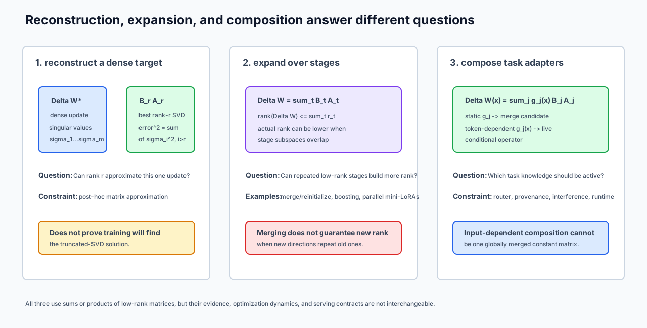
The A22 decomposition taxonomy separates three questions that are often collapsed into one word, rank:

reconstruction
    Can one rank-r matrix approximate one already-defined dense update?

expansion
    Does a sequence of rank-limited stages accumulate new directions?

composition
    What operator results when independently trained updates are added,
    weighted, selected, or routed?

The first question was closed in 0x04. This section owns the second and the static algebraic boundary of the third. M6.9 owns learned routing and serving of multiple adapters.

0x05A Freeze The Composition Object Before Adding Matrices

For stage or task $j$, freeze:

$$B_j\in\mathbb{R}^{m\times r_j}, \qquad A_j\in\mathbb{R}^{r_j\times n}, \qquad \Delta W_j=B_jA_j\in\mathbb{R}^{m\times n}$$

and a scalar coefficient $\lambda_j$. A static composition is:

$$\Delta W_{static} = \sum_{j=1}^{J}\lambda_j\Delta W_j = \sum_{j=1}^{J}\lambda_jB_jA_j$$

The coefficients, factor revisions, target module, orientation, dtype, and merge order are part of the object identity. A sum of adapters trained against different base checkpoints is not automatically a meaningful sum in one common coordinate system.

0x05B Derive The Concatenated Factorization And Its Tighter Rank Bound

Put all output factors side by side and all scaled input factors on top of one another:

$$B_{cat} = \begin{bmatrix}B_1&B_2&\cdots&B_J\end{bmatrix} \in\mathbb{R}^{m\times R}, \qquad A_{cat} = \begin{bmatrix} \lambda_1A_1\\ \lambda_2A_2\\ \vdots\\ \lambda_JA_J \end{bmatrix} \in\mathbb{R}^{R\times n}$$

where $R=\sum_jr_j$. Block multiplication gives:

$$B_{cat}A_{cat} = \sum_{j=1}^{J}\lambda_jB_jA_j = \Delta W_{static}$$

Therefore:

$$\operatorname{rank}(\Delta W_{static}) \leq \min\left( \operatorname{rank}(B_{cat}), \operatorname{rank}(A_{cat}), \sum_jr_j \right)$$

The familiar $\operatorname{rank}(\sum_j\Delta W_j)\leq\sum_jr_j$ bound is only the loosest part. Output-space reuse limits $\operatorname{rank}(B_{cat})$; input-space reuse limits $\operatorname{rank}(A_{cat})$; coefficient cancellation can reduce the final product further.

The exact fixture uses two rank-one updates with coefficients 2 and 3:

$$2f_1e_1^{\top}+3f_2e_2^{\top} = \begin{bmatrix}f_1&f_2\end{bmatrix} \begin{bmatrix}2e_1^{\top}\\3e_2^{\top}\end{bmatrix} = \begin{bmatrix} 2&0&0&0&0&0\\ 0&3&0&0&0&0\\ 0&0&0&0&0&0\\ 0&0&0&0&0&0 \end{bmatrix}$$

Both construction paths reconstruct exactly and the result has rank two.

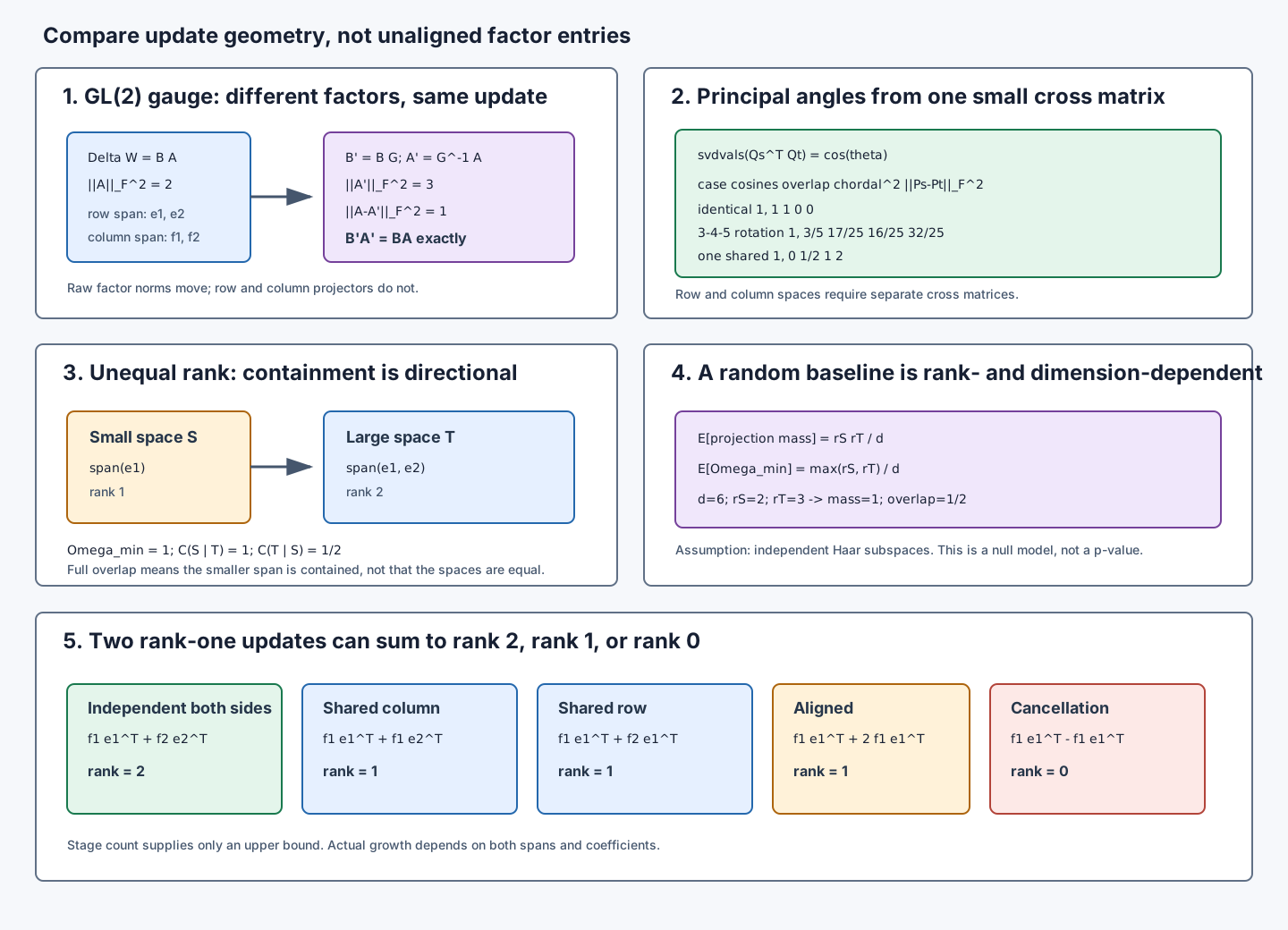
0x05C Why More Stages Do Not Guarantee More Rank

For two rank-one updates $u_1v_1^{\top}$ and $u_2v_2^{\top}$, additive rank growth requires more than a new vector on one side. If $u_2$ is collinear with $u_1$, then:

$$u_1v_1^{\top}+u_1v_2^{\top} = u_1(v_1+v_2)^{\top}$$

and the sum remains rank at most one even when $v_1$ and $v_2$ are independent. The dual statement holds when the row direction is shared:

$$u_1v_1^{\top}+u_2v_1^{\top} = (u_1+u_2)v_1^{\top}$$

For two nonzero rank-one terms, independent left vectors and independent right vectors make the sum rank two. Higher-rank sums can still lose dimensions through cross-term cancellation, so actual rank must be measured after composition.

The executable $4\times6$ ledger makes each boundary explicit:

composition	left update	right update	rank of sum	reason
aligned amplification	$f_1e_1^{\top}$	$2f_1e_1^{\top}$	1	same row and column directions
new row, shared column	$f_1e_1^{\top}$	$f_1e_2^{\top}$	1	$B_{cat}$ has rank one
new column, shared row	$f_1e_1^{\top}$	$f_2e_1^{\top}$	1	$A_{cat}$ has rank one
independent both sides	$f_1e_1^{\top}$	$f_2e_2^{\top}$	2	both concatenated spans expand
exact cancellation	$f_1e_1^{\top}$	$-f_1e_1^{\top}$	0	coefficients cancel the matrix

0x05D Directional Novelty And Destructive Interference Are Different

Subspace novelty asks whether row or column spans expand. Interference asks what the coefficients do inside those spans. The Frobenius norm exposes the cross term:

$$\|\Delta W_1+\Delta W_2\|_F^2 = \|\Delta W_1\|_F^2 + \|\Delta W_2\|_F^2 + 2\langle\Delta W_1,\Delta W_2\rangle_F$$

Positive alignment amplifies. Negative alignment cancels. Orthogonality in matrix Frobenius geometry removes this one cross term, but it does not prove two task objectives are compatible after the updates pass through a nonlinear network. Row-space overlap, column-space overlap, matrix inner product, sampled-output interference, and end-to-end task interference are separate measurements.

0x05E Post-Hoc, Staged, And Joint Composition Are Different Experiments

experiment	what is trained	base seen by later updates	what can be concluded
post-hoc static sum	adapters trained independently	usually the same frozen base	algebraic merge and interference of frozen artifacts
merge and reinitialize	one stage at a time	stage $t+1$ sees the previously merged base	trajectory-dependent rank expansion under an explicit reset policy
jointly trained parallel factors	all factor blocks together	one shared evolving effective operator	coupled optimization under one loss
orthogonality-constrained stages	new stage plus overlap penalty	prior subspaces frozen or referenced	novelty under the selected row, column, or matrix metric
post-hoc SVD compression	no training in the decomposition step	one already-composed matrix	best approximation under the selected residual norm
conditional mixture	router and one or more adapters	input- or token-dependent path	nonlinear/routed operator, not one static merge

Merge-and-reinitialize can fail to expand rank when each stage relearns the same directions. Forcing orthogonality can increase novelty while harming transfer if tasks share useful structure. Joint training can coordinate cancellation or specialization, but its factors are not equivalent to independently trained artifacts merely because their final shapes match.

0x05F Why Input-Dependent Composition Is Not Generally Mergeable

If coefficients depend on the current input:

$$F(x) = \left( W_0+\sum_jg_j(x)\Delta W_j \right)x$$

then $F$ is generally nonlinear even when every $\Delta W_j$ is linear. A one-dimensional exact counterexample needs only:

$$g(x)=x_1, \qquad \Delta W=f_1e_1^{\top}$$

For $x=e_1$, the adapter output is $f_1$. For $2x=2e_1$, it is $4f_1$. Any fixed linear matrix that maps $e_1$ to $f_1$ must map $2e_1$ to $2f_1$, not $4f_1$. Therefore no one constant merged matrix reproduces this gated operator on both inputs.

Special cases can still collapse to a static merge: constant gates, algebraically redundant experts, or a restricted finite input set may admit one equivalent matrix. That is an equivalence to prove, not a default property of routing. M6.9 owns router gradients, task provenance, batching, cache identity, and runtime integration.

0x05G Tensor And Code Trace

def compose_static(adapters, coefficients):
    # Each B_j: [d_out, r_j]; A_j: [r_j, d_in].
    B_cat = concat([B_j for B_j, _ in adapters], axis=1)
    A_cat = concat([
        coefficient * A_j
        for coefficient, (_, A_j) in zip(coefficients, adapters)
    ], axis=0)

    delta_from_factors = B_cat @ A_cat
    delta_from_sum = sum(
        coefficient * (B_j @ A_j)
        for coefficient, (B_j, A_j) in zip(coefficients, adapters)
    )
    assert_close(delta_from_factors, delta_from_sum)
    return delta_from_sum

For staged expansion, persist the update matrix or a rank-revealing decomposition at every stage. Comparing only current factors is insufficient because factor gauge can change without changing the update.

for stage in stages:
    delta_stage = reconstruct_adapter(stage.B, stage.A)
    delta_total = delta_total + stage.coefficient * delta_stage

    report({
        "rank_stage": numerical_rank(delta_stage, tolerance),
        "rank_total": numerical_rank(delta_total, tolerance),
        "row_basis": right_singular_basis(delta_total, tolerance),
        "column_basis": left_singular_basis(delta_total, tolerance),
        "task_metrics": evaluate_target_and_retention(model, delta_total),
    })

The tolerance, decomposition backend, coefficient dtype, accumulation dtype, base revision, and stage order belong in the artifact manifest.

0x05H Composition Alternatives And Failure Boundaries

design	useful when	failure boundary
sum merged matrices	coefficients are static and artifacts share one base contract	destructive cancellation or rank growth beyond release budget
concatenate factors without dense merge	runtime supports a larger live adapter	extra adapter FLOPs and memory scale with total factor width
compress composed matrix by SVD	one static release needs a lower rank	reconstruction loss can erase task-specific directions
orthogonalize new stage	novelty is explicitly desired	shared useful directions are suppressed
select one adapter	tasks are separable and identity is known	selector error and fragmented batching
mix adapters with dynamic gates	inputs benefit from conditional sharing	no global merge; routing and provenance become runtime state

0x06 Subspace Similarity, Principal Angles, And The LoRA Experiment

Subspace comparison must answer four questions before reporting one scalar:

Which matrix object is decomposed?
Is the input-side row space or output-side column space compared?
How is numerical rank selected?
Does the normalization mean similarity, containment, or directed coverage?

Without those fields, a heatmap can be visually precise and mathematically ambiguous.

0x06A Raw Factor Entries Are Not Gauge-Invariant Objects

Take the exact rank-two update:

$$B= \begin{bmatrix} 5&0\\0&2\\0&0\\0&0 \end{bmatrix}, \qquad A= \begin{bmatrix} 1&0&0&0&0&0\\ 0&1&0&0&0&0 \end{bmatrix}$$

and the invertible coordinate change:

$$G= \begin{bmatrix}1&1\\0&1\end{bmatrix}, \qquad G^{-1}= \begin{bmatrix}1&-1\\0&1\end{bmatrix}$$

Define $B'=BG$ and $A'=G^{-1}A$. Then:

$$B'A'=BGG^{-1}A=BA$$

but the raw factor diagnostics change:

$$\|A\|_F^2=2, \qquad \|A'\|_F^2=3, \qquad \|A-A'\|_F^2=1$$

Scaling $G=\operatorname{diag}(c,c^{-1})$ can make factor norms vary arbitrarily while preserving the product. Entrywise distance, factor cosine, and unaligned factor norms therefore do not define an intrinsic distance between LoRA updates.

0x06B Extract Gauge-Invariant Row And Column Bases

For one reconstructed update with numerical rank $r$:

$$\Delta W = U_r\Sigma_rV_r^{\top}$$

define:

$$Q_{col}=U_r\in\mathbb{R}^{m\times r}, \qquad Q_{row}=V_r\in\mathbb{R}^{n\times r}$$

and projectors:

$$P_{col}=Q_{col}Q_{col}^{\top}, \qquad P_{row}=Q_{row}Q_{row}^{\top}$$

The bases can rotate inside a repeated-singular-value subspace, but the projectors remain unchanged. At full factor rank, $\operatorname{col}(BA)=\operatorname{col}(B)$ and $\operatorname{row}(BA)=\operatorname{row}(A)$. Under rank collapse, those equalities can shrink, so decomposing $BA$ is safer than assuming configured factor width equals learned update rank.

A rank-revealing QR can extract a span without a full SVD. The SVD is still needed when comparison means leading energy-ordered directions rather than the complete numerical span.

0x06C Derive Principal Angles From One Cross Matrix

Let $Q_S\in\mathbb{R}^{d\times r_S}$ and $Q_T\in\mathbb{R}^{d\times r_T}$ have orthonormal columns, and let $p=\min(r_S,r_T)$. The first principal angle solves:

$$\cos\theta_1 = \max_{\substack{s\in S,\ t\in T\\\|s\|_2=\|t\|_2=1}} s^{\top}t$$

Write $s=Q_Sa$ and $t=Q_Tb$. The objective becomes:

$$a^{\top}(Q_S^{\top}Q_T)b$$

over unit $a$ and $b$, whose maximum is the largest singular value of the cross matrix. Constraining later vectors to be orthogonal to earlier principal vectors recursively yields:

$$Q_S^{\top}Q_T = L\operatorname{diag}(\sigma_1,\ldots,\sigma_p)R^{\top}, \qquad \sigma_a=\cos\theta_a, \qquad 0\leq\theta_a\leq\frac{\pi}{2}$$

This is the QR-then-SVD numerical contract developed by Björck and Golub: rank-reveal the input spans, orthonormalize them, then decompose the small cross matrix. Computing an SVD directly on arbitrary raw factors measures factor scaling and conditioning as well as span geometry.

0x06D Derive Projection Overlap, Chordal Distance, And Projector Distance

Because the squared Frobenius norm is the sum of squared singular values:

$$M(S,T) = \|Q_S^{\top}Q_T\|_F^2 = \sum_{a=1}^{p}\cos^2\theta_a$$

The original LoRA normalization is:

$$\Omega_{min}(S,T) = \frac{M(S,T)}{p} \in[0,1]$$

The squared chordal/projection distance used by that normalization is:

$$d_{chord}^2(S,T) = \sum_{a=1}^{p}\sin^2\theta_a = p-M(S,T)$$

Therefore the correct normalized identity is:

$$\Omega_{min}(S,T) = 1-\frac{d_{chord}^2(S,T)}{p}$$

Projector distance keeps unequal-rank surplus dimensions visible:

$$\begin{aligned} \|P_S-P_T\|_F^2 &=\operatorname{tr}(P_S)+\operatorname{tr}(P_T)-2\operatorname{tr}(P_SP_T)\\ &=r_S+r_T-2M(S,T) \end{aligned}$$

For equal rank $r$, this reduces to $2d_{chord}^2$. For unequal ranks it also charges the dimensions that have no paired principal angle.

0x06E Exact Principal-Angle Ledger

The immutable fixture compares the base row space $\operatorname{span}(e_1,e_2)$ with four alternatives. The $3$-$4$-$5$ case uses:

$$Q_T= \begin{bmatrix} \frac35&0\\ 0&1\\ \frac45&0\\ 0&0\\ 0&0\\ 0&0 \end{bmatrix}, \qquad Q_S^{\top}Q_T= \begin{bmatrix}\frac35&0\\0&1\end{bmatrix}$$

so the principal cosines are $(1,3/5)$ and the angles are $(0,\arccos(3/5))$.

row-space case	principal cosines	$\Omega_{min}$	$d_{chord}^2$	$\|P_S-P_T\|_F^2$
identical	$(1,1)$	$1$	$0$	$0$
$3$-$4$-$5$ rotation	$(1,3/5)$	$17/25$	$16/25$	$32/25$
one shared direction	$(1,0)$	$1/2$	$1$	$2$
orthogonal	$(0,0)$	$0$	$2$	$4$

These are exact rational checks, not rounded output from a numerical SVD. A production run must additionally record decomposition backend, dtype, singular-value cutoff, convergence status, and ordering/tie policy.

0x06F Row And Column Spaces Answer Different Questions

For $\Delta W:\mathbb{R}^{n}\rightarrow\mathbb{R}^{m}$:

row space in R^n
    Which input directions can the update read or distinguish?

column space in R^m
    Which output directions can the update write?

The fixture’s column_partial case has identical row spaces but only one shared output direction:

row principal cosines       = (1, 1), overlap = 1
column principal cosines    = (1, 0), overlap = 1/2

One score cannot substitute for the other. Comparing only the down-factor row space can miss a changed output builder; comparing only the up-factor column space can miss changed input features.

0x06G Min-Rank Normalization Means Containment, Not Equality

Let:

$$S=\operatorname{span}(e_1), \qquad T=\operatorname{span}(e_1,e_2)$$

Then $M(S,T)=1$ and $p=1$, so:

$$\Omega_{min}(S,T)=1$$

The score correctly says the smaller subspace is fully contained in the larger. It does not say the spaces are equal. Directed coverage keeps both statements:

$$C(S\mid T) = \frac{M(S,T)}{r_S}, \qquad C(T\mid S) = \frac{M(S,T)}{r_T}$$

For this example:

$$C(S\mid T)=1, \qquad C(T\mid S)=\frac12$$

Always report both directed coverages when retained ranks differ. Alternatively, report projector distance, which charges the unmatched dimension automatically.

0x06H A Random Baseline Depends On Ambient Dimension And Rank

A raw overlap value has no rank-free random baseline. For independent Haar-distributed subspaces with ranks $r_S,r_T$ in $\mathbb{R}^{d}$, rotational symmetry gives:

$$\mathbb{E}[P_T]=\frac{r_T}{d}I$$

Hence:

$$\begin{aligned} \mathbb{E}[M(S,T)] &=\mathbb{E}[\operatorname{tr}(P_SP_T)]\\ &=\operatorname{tr}\left(P_S\frac{r_T}{d}I\right)\\ &=\frac{r_Sr_T}{d} \end{aligned}$$

and:

$$\mathbb{E}[\Omega_{min}] = \frac{\max(r_S,r_T)}{d}$$

For $d=6$, $r_S=2$, and $r_T=3$, the expected projection mass is one and the normalized overlap is $1/2$. A heatmap cell of $0.5$ can therefore be strong or unremarkable depending on ambient dimension, retained ranks, and null model. Learned subspaces are not Haar random; the formula is a baseline contract, not a p-value.

0x06I Procrustes Aligns Basis Coordinates Only After Span Extraction

Two orthonormal bases of the same subspace can differ by an orthogonal coordinate rotation. For equal rank, solve:

$$R^* = \arg\min_{R^{\top}R=I} \|Q_S-Q_TR\|_F^2$$

If:

$$Q_T^{\top}Q_S=L\Sigma R_0^{\top}$$

then the orthogonal Procrustes solution is $R^*=LR_0^{\top}$, and:

$$\min_R\|Q_S-Q_TR\|_F^2 = 2r-2\sum_a\cos\theta_a$$

The fixture rotates the basis of $\operatorname{span}(e_1,e_2)$ by 90 degrees. Its raw basis difference is four, its projector difference is zero, and its aligned difference is zero.

This procedure begins after QR or SVD has produced orthonormal bases. It does not solve arbitrary $GL(r)$ gauge in raw LoRA factors. Projectors and principal angles remain the primary invariant diagnostics; aligned bases are useful only when direction-by-direction correspondence is needed.

0x06J What The Original LoRA Experiment Actually Compares

The original LoRA paper’s Section 7.2 and Appendix G compare the leading right singular-vector directions of learned down factors $A_{r=8}$ and $A_{r=64}$ in selected GPT-3 attention projections. These vectors live in the common input ambient space even though the two factor matrices have different configured ranks. The paper notes that an analogous left-singular analysis can be done for $B$.

$$\phi(A_{8},A_{64},i,j) = \frac{ \left\| (Q_{A_8}^{i})^{\top}Q_{A_{64}}^{j} \right\|_F^2 }{\min(i,j)}$$

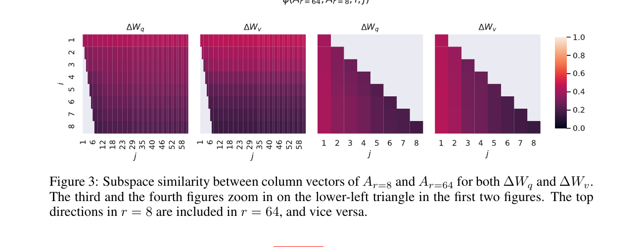
Source: LoRA, Figure 3. The source reports that the leading directions for the rank-8 and rank-64 factors overlap in the tested layer and that one shared direction has normalized similarity above 0.5 for the shown query/value cases. The paper also compares rank-64 runs across seeds and random Gaussian matrices. These are source-reported experiments, not reproduced measurements here.

The distinction between factor row space and update row space matters. If $B$ has full column rank, $\operatorname{row}(BA)=\operatorname{row}(A)$. If $B$ collapses rank, some directions in $A$ do not survive into $BA$. A modern replication should report both factor-space and reconstructed-update diagnostics rather than silently treating them as identical.

0x06K Executable Tensor Trace

def subspace_report(delta_left, delta_right, tolerance):
    # Both updates are [d_out, d_in] and share the same module identity.
    U_l, s_l, Vh_l = svd(delta_left, full_matrices=False)
    U_r, s_r, Vh_r = svd(delta_right, full_matrices=False)

    rank_l = count(s_l > tolerance * s_l[0])
    rank_r = count(s_r > tolerance * s_r[0])

    Qcol_l = U_l[:, :rank_l]                 # [d_out, rank_l]
    Qcol_r = U_r[:, :rank_r]                 # [d_out, rank_r]
    Qrow_l = Vh_l[:rank_l, :].T              # [d_in, rank_l]
    Qrow_r = Vh_r[:rank_r, :].T              # [d_in, rank_r]

    def compare(Q_l, Q_r):
        cross = Q_l.T @ Q_r                  # [rank_l, rank_r]
        cosines = svdvals(cross)              # length min(rank_l, rank_r)
        mass = sum(cosines * cosines)
        p = min(Q_l.shape[1], Q_r.shape[1])

        return {
            "principal_cosines": cosines,
            "principal_angles": arccos(clip(cosines, 0, 1)),
            "min_rank_overlap": mass / p,
            "left_covered_by_right": mass / Q_l.shape[1],
            "right_covered_by_left": mass / Q_r.shape[1],
            "chordal_squared": p - mass,
            "projector_distance_squared": (
                Q_l.shape[1] + Q_r.shape[1] - 2 * mass
            ),
        }

    return {
        "row": compare(Qrow_l, Qrow_r),
        "column": compare(Qcol_l, Qcol_r),
    }

Near one, clip principal cosines only after recording the unclipped floating-point excess. A value such as $1+10^{-7}$ is a numerical symptom, not a physical angle. Rank-zero updates need an explicit policy because min-rank normalization would divide by zero.

0x06L A Reproducible Subspace Protocol

1. Freeze base checkpoint, target module, factor orientation, adapter revision,
   dataset, seed, optimizer, step, and merge state.
2. Reconstruct the exact update matrix in a named accumulation dtype.
3. Select algebraic or numerical rank with an explicit threshold and tie rule.
4. Extract both row and column orthonormal bases.
5. Compute principal cosines from the small cross matrix.
6. Emit angles, projection mass, min-rank overlap, both directed coverages,
   chordal distance, and projector distance.
7. Add a rank- and ambient-dimension-matched random baseline.
8. Report matrix inner products and sampled-output interference separately.
9. Evaluate target, retention, and stress metrics before claiming compatibility.
10. Preserve all artifacts needed to rerun the decomposition.

The immutable Loop 2 protocol already required principal angles and normalized overlap. Loop 6 makes the basis, rank, side, coverage, and null-model fields executable instead of changing that historical contract.

0x06M What Similarity Does And Does Not Prove

observation	supported interpretation	unsupported leap
$\Omega_{min}=1$ at equal ranks	the two numerical subspaces coincide	the update magnitudes or task effects coincide
$\Omega_{min}=1$ at unequal ranks	the smaller span is contained in the larger	the larger has no additional directions
low row overlap	updates read different input directions	tasks cannot transfer
low column overlap	updates write different output directions	their end-to-end outputs never interfere
high overlap across stages	stages reuse directions	the matrix sum has identical coefficients or quality
high overlap across seeds	stable span under the tested protocol	universal intrinsic rank
low random-baseline-adjusted overlap	more separation than the chosen null	statistical significance without a sampling protocol

The original LoRA result does not establish that every task has rank one, every layer has the same useful rank, rank-64 tails are useless, another optimizer learns the same directions, or intrinsic dimension $d_{90}$ equals a shared matrix-subspace dimension. It supports a narrower source-reported conclusion: leading factor directions were shared across some tested ranks and seeds while low configured ranks remained competitive in those experiments.

0x07 Initialization Is An Optimization Contract, Not A Zero-Product Trick

M6.3 owns the implemented LoRA operator, its tensor shapes, and its local backward pass. This section consumes that closed contract and asks a different question:

Once two factors represent the same initial update, what motion does the optimizer induce in the represented matrix?

The answer requires freezing more than $\Delta W_0$. A reproducible dynamics statement must name:

product order and factor shapes
which factor entries are random, zero, or structured
factor-entry variance as width and rank change
adapter scale s
learning rate for each factor
simultaneous or sequential factor updates
optimizer state, epsilon, clipping, and decay
factor and optimizer-state dtypes

The exact Loop 7 fixture uses $d_{in}=d_{out}=r=2$, $\Delta=sBA$, one frozen dense gradient $G$, exact rational arithmetic, and simultaneous plain-SGD gradients evaluated at the same old factor state. It is a local algebra oracle, not a model-training experiment.

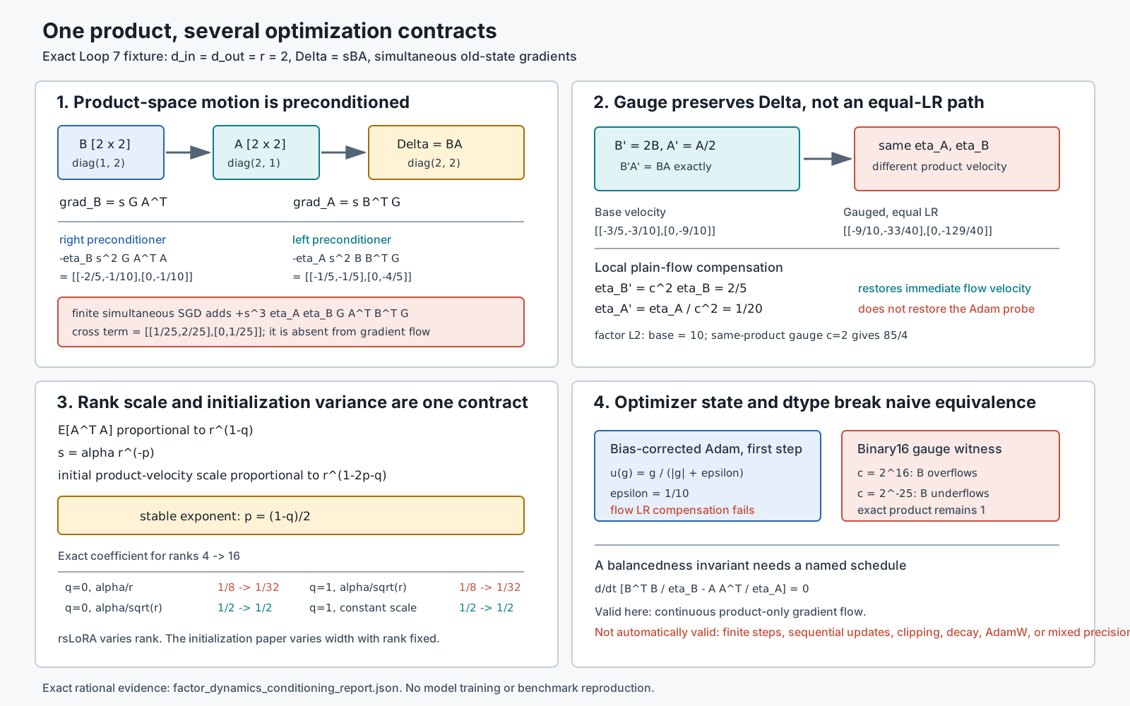
0x07A Derive The Factor Gradients From One Differential

Let:

$$W_{eff}=W+\Delta, \qquad \Delta=sBA$$

with:

$$B\in\mathbb{R}^{d_{out}\times r}, \qquad A\in\mathbb{R}^{r\times d_{in}}, \qquad G=\frac{\partial\mathcal{L}}{\partial W_{eff}} \in\mathbb{R}^{d_{out}\times d_{in}}.$$

The differential of the product is:

$$d\Delta=s\left(dB\,A+B\,dA\right).$$

Using the Frobenius inner product:

$$d\mathcal{L} = \langle G,d\Delta\rangle_F = s\langle GA^{\top},dB\rangle_F + s\langle B^{\top}G,dA\rangle_F.$$

Therefore:

$$\boxed{ \nabla_B\mathcal{L}=sGA^{\top} }$$

and:

$$\boxed{ \nabla_A\mathcal{L}=sB^{\top}G }.$$

The formulas are reciprocal. The current scale and orientation of $A$ determine the gradient seen by $B$; the current scale and orientation of $B$ determine the gradient seen by $A$.

0x07B Derive Motion In Product Space

Under continuous plain gradient flow with factor-specific rates $\eta_B$ and $\eta_A$:

$$\dot B=-\eta_B sGA^{\top}, \qquad \dot A=-\eta_A sB^{\top}G.$$

Differentiate the represented update rather than either factor:

$$\dot\Delta = s\left(\dot B A+B\dot A\right).$$

Substitution gives:

$$\boxed{ \dot\Delta = -s^2\left( \eta_B G A^{\top}A + \eta_A BB^{\top}G \right) }.$$

This is not ordinary dense gradient descent $-\eta G$ on $\Delta$. Factorization inserts two state-dependent operators:

Term	Acts on	Geometric role
$GA^{\top}A$	input side of $G$	right preconditioning by the row geometry of $A$
$BB^{\top}G$	output side of $G$	left preconditioning by the column geometry of $B$

At a zero-$B$ start only the right-preconditioned path exists. At a zero-$A$ start only the left-preconditioned path exists. Once both factors move, the two paths interact.

0x07C Exact Tensor Trace

Freeze:

$$G= \begin{bmatrix} 1&1\\ 0&1 \end{bmatrix}, \quad B= \begin{bmatrix} 1&0\\ 0&2 \end{bmatrix}, \quad A= \begin{bmatrix} 2&0\\ 0&1 \end{bmatrix},$$ $$s=1, \qquad \eta_B=\frac{1}{10}, \qquad \eta_A=\frac{1}{5}.$$

Then:

$$BA= \begin{bmatrix} 2&0\\ 0&2 \end{bmatrix}, \qquad \nabla_B\mathcal{L}= \begin{bmatrix} 2&1\\ 0&1 \end{bmatrix}, \qquad \nabla_A\mathcal{L}= \begin{bmatrix} 1&1\\ 0&2 \end{bmatrix}.$$

The two product-space contributions are:

$$-\eta_BGA^{\top}A = \begin{bmatrix} -2/5&-1/10\\ 0&-1/10 \end{bmatrix}$$

and:

$$-\eta_ABB^{\top}G = \begin{bmatrix} -1/5&-1/5\\ 0&-4/5 \end{bmatrix}.$$

Thus:

$$\dot\Delta= \begin{bmatrix} -3/5&-3/10\\ 0&-9/10 \end{bmatrix}.$$

The exact fixture recomputes every entry from the factors. The values are not copied from a paper table.

0x07D A Simultaneous Finite Step Has An Extra Product Term

For simultaneous old-state SGD:

$$B^+=B-\eta_BsGA^{\top}, \qquad A^+=A-\eta_AsB^{\top}G.$$

Expanding $sB^+A^+$ gives:

$$\boxed{ \Delta^+-\Delta = -\eta_Bs^2GA^{\top}A -\eta_As^2BB^{\top}G +\eta_A\eta_Bs^3GA^{\top}B^{\top}G }.$$

The first two terms are the Euler approximation to the continuous flow. The third is a finite-step multiplicative cross term. In the exact trace:

$$\eta_A\eta_BGA^{\top}B^{\top}G = \begin{bmatrix} 1/25&2/25\\ 0&1/25 \end{bmatrix}.$$

Therefore:

$$\Delta^+-\Delta = \begin{bmatrix} -14/25&-11/50\\ 0&-43/50 \end{bmatrix}.$$

An implementation that updates $B$, recomputes $\nabla_A$ from the new $B$, and then updates $A$ executes a different sequential algorithm. The distinction is not an implementation footnote: it changes the finite-step map.

0x07E Derive The Weighted Gram Invariant And Its Scope

Both $B^{\top}B$ and $AA^{\top}$ are $r\times r$ latent-coordinate Gram matrices. Under the frozen continuous flow above:

$$\frac{d}{dt}(B^{\top}B) = -\eta_Bs\left(AG^{\top}B+B^{\top}GA^{\top}\right)$$

and:

$$\frac{d}{dt}(AA^{\top}) = -\eta_As\left(B^{\top}GA^{\top}+AG^{\top}B\right).$$

Divide by the corresponding learning rates and subtract:

$$\boxed{ \frac{d}{dt} \left( \frac{B^{\top}B}{\eta_B} - \frac{AA^{\top}}{\eta_A} \right) =0 }.$$

For the exact trace, the conserved matrix is:

$$\frac{B^{\top}B}{\eta_B} - \frac{AA^{\top}}{\eta_A} = \begin{bmatrix} -10&0\\ 0&35 \end{bmatrix}.$$

This local derivation is related to the balancedness lineage for homogeneous factorizations in Du, Hu, and Lee (NeurIPS 2018). It does not establish that the same matrix is conserved by finite steps, sequential updates, clipping, factor decay, adaptive moments, stochastic rounding, or arbitrary mixed-precision LoRA code.

0x07F Four Zero-Product Mechanisms

The statement "$\Delta_0=0$" hides different derivative states.

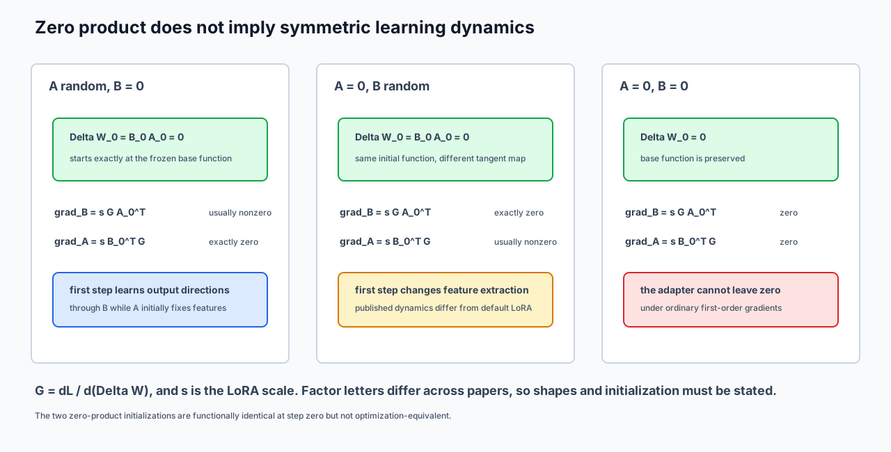
Standard: random $A_0$, zero $B_0$

$$\Delta_0=0, \qquad \nabla_B\mathcal{L}=sGA_0^{\top}, \qquad \nabla_A\mathcal{L}=0.$$

The first product motion is:

$$\dot\Delta_0=-\eta_Bs^2GA_0^{\top}A_0.$$

$A_0$ is initially a fixed input-side feature map. This is the initialization specified by the original LoRA paper: random Gaussian $A$, zero $B$, and therefore zero initial adapter output.

Reversed: zero $A_0$, random $B_0$

$$\Delta_0=0, \qquad \nabla_B\mathcal{L}=0, \qquad \nabla_A\mathcal{L}=sB_0^{\top}G,$$

with:

$$\dot\Delta_0=-\eta_As^2B_0B_0^{\top}G.$$

The initial function is identical to the standard start, but the first gradient is projected on the output side instead of the input side.

Both factors zero

$$A_0=B_0=0 \quad\Longrightarrow\quad \nabla_A\mathcal{L}=\nabla_B\mathcal{L}=0.$$

Ordinary first-order optimization cannot leave this point.

Both factors nonzero but $B_0A_0=0$

Zero product does not imply a zero factor. For example:

$$B_0= \begin{bmatrix} 1&0\\ 0&0 \end{bmatrix}, \qquad A_0= \begin{bmatrix} 0&0\\ 0&1 \end{bmatrix}$$

gives $B_0A_0=0$, yet the exact fixture obtains:

$$\nabla_B\mathcal{L}= \begin{bmatrix} 0&1\\ 0&1 \end{bmatrix}, \qquad \nabla_A\mathcal{L}= \begin{bmatrix} 1&1\\ 0&0 \end{bmatrix}.$$

Both factors can move immediately. A zero function perturbation, a zero factor, and a dead first-order state are three different claims.

0x07G The Initialization Paper Varies Width, Not Rank

The Impact of Initialization on LoRA Finetuning Dynamics compares two zero-product paths under a specific asymptotic contract:

Paper notation	Random factor	Zero factor	Asymptotic variable
Init[$A$]	$A$ with entry variance $\Theta(n^{-1})$	$B$	model width $n\to\infty$, rank fixed
Init[$B$]	$B$ with entry variance $\Theta(r^{-1})$	$A$	model width $n\to\infty$, rank fixed

Using the paper’s learning-rate exponent notation, its analysis reports:

Init[A]: stable when gamma[eta] <= -1/2
         efficient feature learning at gamma[eta] = -1/2

Init[B]: stable when gamma[eta] <= -1
         cannot efficiently train both factors in that asymptotic setup

Those are theorem-scoped statements. They do not establish a universal finite-width learning rate, optimizer-independent superiority, or a rank-scaling law.

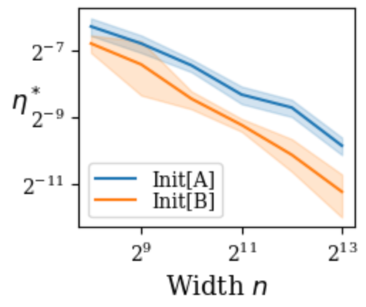
Source-reported evidence: Figure 2 from “The Impact of Initialization on LoRA Finetuning Dynamics,” arXiv:2406.08447v1, extracted without redrawing under the paper’s CC BY 4.0 license. The paper reports that the selected learning rate decreases with width and differs between Init[$A$] and Init[$B$] in its experiment. This repository did not reproduce the runs.

0x07H Tensor And Optimizer Trace

The gradient calculation and the factor update must be separate operations:

def factor_gradients(B, A, G, scale):
    grad_B = scale * (G @ A.T)
    grad_A = scale * (B.T @ G)
    return grad_B, grad_A


# Both gradients read the same old factor state.
grad_B, grad_A = factor_gradients(B, A, G, scale)

B_next = optimizer_B.step(B, grad_B)
A_next = optimizer_A.step(A, grad_A)

delta_before = scale * (B @ A)
delta_after = scale * (B_next @ A_next)
product_step = delta_after - delta_before

For diagnostics, record both the factor-space and product-space quantities:

diagnostics = {
    "norm_A": frobenius_norm(A),
    "norm_B": frobenius_norm(B),
    "norm_grad_A": frobenius_norm(grad_A),
    "norm_grad_B": frobenius_norm(grad_B),
    "norm_product": frobenius_norm(scale * (B @ A)),
    "norm_product_step": frobenius_norm(product_step),
    "right_gram": A.T @ A,
    "left_gram": B @ B.T,
    "latent_balance": B.T @ B / eta_B - A @ A.T / eta_A,
}

The final line is a diagnostic under a named plain-flow comparison. It is not an assertion that a practical optimizer must conserve it.

0x07I Factor Letters Are Not An Interface

Some papers and libraries swap the letters used for the down and up projections. A statement such as “initialize $A$ to zero” is therefore not portable. State the full ABI:

down factor: [r, d_in]
up factor: [d_out, r]
product order: up @ down
zero factor: up or down
random-factor distribution and variance
stored scaling and factor-specific optimizer groups

M6.3 owns the checkpoint and merge implementation of that ABI. M6.7 owns the consequence: changing any one field can change the trajectory even when the step-zero product is unchanged.

0x08 Factor Gauge, Scaling, Optimizers, And Conditioning

0x08A Feature Extractor And Output Builder Are Source-Scoped Roles

For $BAx$, $A$ maps an input into $r$ latent coordinates and $B$ maps those coordinates into the output space. Asymmetry in Low-Rank Adapters of Foundation Models studies this distinction and reports settings in which freezing a random projection factor while training the output-building factor remains competitive.

That result does not make one factor universally disposable. It depends on the paper’s random-feature assumptions, models, tasks, ranks, and optimization protocol. If the fixed input projection omits task-relevant directions, training only $B$ cannot create them.

0x08B Gauge-Equivalent Factors Need Not Follow Gauge-Equivalent Paths

For nonzero scalar $c$:

$$B'=cB, \qquad A'=\frac{A}{c}, \qquad B'A'=BA.$$

But the Gram operators become:

$$A'^{\top}A'=\frac{1}{c^2}A^{\top}A, \qquad B'B'^{\top}=c^2BB^{\top}.$$

With unchanged factor learning rates:

$$\dot\Delta' = -s^2\left( \frac{\eta_B}{c^2}GA^{\top}A + c^2\eta_ABB^{\top}G \right).$$

The exact fixture uses $c=2$. The product remains $\operatorname{diag}(2,2)$, but the equal-rate velocity changes from:

$$\begin{bmatrix} -3/5&-3/10\\ 0&-9/10 \end{bmatrix}$$

to:

$$\begin{bmatrix} -9/10&-33/40\\ 0&-129/40 \end{bmatrix}.$$

Loop 4 established that gauge-equivalent factors represent one matrix. Loop 7 establishes the complementary fact: Euclidean factor optimization is coordinate-dependent.

0x08C A Local Plain-Flow Gauge Compensation

To preserve the two coefficients in the immediate continuous flow after $B'=cB$, $A'=A/c$, choose:

$$\boxed{ \eta_B'=c^2\eta_B, \qquad \eta_A'=\frac{\eta_A}{c^2} }.$$

For $c=2$:

$$\eta_B'=\frac{2}{5}, \qquad \eta_A'=\frac{1}{20},$$

and the exact immediate product velocity matches the base velocity.

The compensation also holds for finite plain-SGD steps, not only for the immediate velocity. Under the gauge, $\nabla_{B'}\mathcal{L}=\nabla_B\mathcal{L}/c$ and $\nabla_{A'}\mathcal{L}=c\nabla_A\mathcal{L}$, so one simultaneous step with the compensated rates gives:

$$B'^+=cB-c^2\eta_B\frac{\nabla_B\mathcal{L}}{c}=cB^+, \qquad A'^+=\frac{A}{c}-\frac{\eta_A}{c^2}\,c\nabla_A\mathcal{L}=\frac{A^+}{c}.$$

The new factors are again gauge-equivalent, so $B'^+A'^+=B^+A^+$. The multiplicative cross term of 0x07D is included: $\eta_A'\eta_B'=\eta_A\eta_B$, and the $1/c$ and $c$ gradient scales cancel. In the exact trace both parameterizations reach:

$$\Delta^+= \begin{bmatrix} 36/25&-11/50\\ 0&57/50 \end{bmatrix}.$$

Because $G$ depends only on the product, the next gradient is the same in both runs, and the argument repeats at every step. Plain SGD with compensated rates therefore follows the same product trajectory; only operations that act on factor coordinates break the match:

factor clipping thresholds are coordinate-dependent
factor decay is coordinate-dependent
adaptive moments carry their own coordinate history
finite-precision range depends on factor magnitude

0x08D Why The Compensation Does Not Transfer To Adam

At the first bias-corrected Adam step from zero moments, ignoring weight decay:

$$\widehat m=g, \qquad \widehat v=g^2,$$

so each coordinate uses:

$$u(g)=\frac{g}{|g|+\epsilon}.$$

Under the scalar gauge, $\nabla_B$ scales by $1/c$ while $\nabla_A$ scales by $c$. The additive $\epsilon$ prevents these directions from being homogeneous rescalings. Even before later moment history appears, the plain-flow learning-rate compensation is no longer an optimizer equivalence.

With $\epsilon=1/10$, the exact oracle obtains:

$$\Delta^+_{base} = \begin{bmatrix} 380/231&-5/21\\ 0&17/11 \end{bmatrix}$$

but the compensated gauged factors produce:

$$\Delta^+_{gauge} = \begin{bmatrix} 120/77&-4325/18942\\ 0&407/246 \end{bmatrix}.$$

They are not equal. This one-step counterexample does not characterize long-run AdamW behavior; it disproves a simpler and commonly implied claim that a plain-SGD gauge compensation automatically transfers to an adaptive optimizer.

0x08E Factor Decay Is Not Product Decay

A factor penalty:

$$R(A,B)=\|A\|_F^2+\|B\|_F^2$$

becomes, under the scalar gauge:

$$R(A/c,cB) = c^{-2}\|A\|_F^2+c^2\|B\|_F^2.$$

Although $BA$ is unchanged, the penalty is not. Its balancing gauge satisfies:

$$c^4=\frac{\|A\|_F^2}{\|B\|_F^2}.$$

In the exact case, the base penalty is $10$ and the same-product $c=2$ penalty is $85/4$. Applying L2 regularization or decoupled weight decay to factors therefore chooses a factor gauge as well as constraining magnitude. It is not equivalent to regularizing $\|BA\|_F^2$.

0x08F Derive Rank Scaling Together With Initialization Variance

At the standard $B_0=0$ start:

$$\dot\Delta_0=-\eta_Bs^2GA_0^{\top}A_0.$$

Suppose the $r$ rows of $A_0$ are independent, zero mean, and have coordinate covariance:

$$\mathbb{E}[a_ia_i^{\top}]=\sigma_A^2I.$$

Then:

$$\mathbb{E}[A_0^{\top}A_0]=r\sigma_A^2I$$

and:

$$\boxed{ \mathbb{E}[\dot\Delta_0] = -\eta_Bs^2r\sigma_A^2G }.$$

The first $B$-gradient moment obeys the matching dependence:

$$\mathbb{E}\|\nabla_B\mathcal{L}\|_F^2 = s^2r\sigma_A^2\|G\|_F^2.$$

Parameterize both choices:

$$s=\alpha r^{-p}, \qquad \sigma_A^2=\kappa r^{-q}.$$

The rank exponent of the initial product velocity is:

$$s^2r\sigma_A^2 = \alpha^2\kappa r^{1-2p-q}.$$

Rank-independent scale requires:

$$\boxed{ p=\frac{1-q}{2} }.$$

This derivation explains why a scaling rule cannot be judged independently of factor initialization:

Initialization variance	$q$	Stable exponent $p$	Corresponding scale
factor-entry variance independent of rank	0	$1/2$	$\alpha/\sqrt r$
factor-entry variance proportional to $1/r$	1	0	constant $\alpha$

rsLoRA analyzes the first regime and motivates $\alpha/\sqrt r$ under its stated assumptions. The result is not assumption-free and does not say that every existing initialization must use the same scale.

0x08G Exact Rank Ledger

The exact fixture repeats rows $e_1,e_2$ and compares ranks $4$ and $16$. Its row-coordinate second moment is $1/2$.

Factor normalization	Scale	Coefficient at $r=4$	Coefficient at $r=16$	Trend
rank-independent rows, $q=0$	$\alpha/r$	$1/8$	$1/32$	shrinks
rank-independent rows, $q=0$	$\alpha/\sqrt r$	$1/2$	$1/2$	stable
rows divided by $\sqrt r$, $q=1$	$\alpha/\sqrt r$	$1/8$	$1/32$	shrinks
rows divided by $\sqrt r$, $q=1$	constant $\alpha$	$1/2$	$1/2$	stable

The table is not a quality benchmark. It verifies one initial product-velocity coefficient exactly.

0x08H Rank Asymptotics And Width Asymptotics Are Different Experiments

Two primary sources vary different axes:

Source	Varies	Holds fixed or assumes	Supports
initialization dynamics, arXiv:2406.08447v1	model width $n$	rank fixed; source-specific variance and LR exponents	width-dependent stability and feature-learning analysis
rsLoRA, arXiv:2312.03732v1	adapter rank $r$	source-specific initialization moments and optimization assumptions	rank-dependent adapter scaling

One cannot substitute $n$ for $r$ in either theorem. A practical sweep may vary both, but then it is a third protocol and must report both variance rules and both scale rules.

0x08I Dtype Feasibility Is Gauge-Dependent

In exact arithmetic:

$$1\cdot1 = 2^{16}\cdot2^{-16} = 2^{-25}\cdot2^{25} =1.$$

If those coordinates are stored directly in IEEE binary16:

largest finite value: 65504
smallest positive subnormal: 2^-24

c = 2^16:
    B' = 65536 is above the finite range

c = 2^-25:
    B' is below the smallest subnormal
    A' = 2^25 is above the finite range

The product is mathematically identical, but the factor representation is not equally storable. This is a coordinate witness, not a claim that every LoRA run stores master factors or optimizer state in binary16. M6.3 owns the actual mixed-precision state contract; M8 owns general numerical representation.

0x08J Alternative Factor-Training Designs

The derivations expose several genuinely different choices:

Design	Trainable state	Initial product path	Benefit sought	Main limitation
random $A$, zero $B$, train both	both factors	right-preconditioned first motion	standard zero-output start and later feature learning	asymmetric early dynamics
zero $A$, random $B$, train both	both factors	left-preconditioned first motion	reverse output-side start	narrower stable-rate regime in the cited width analysis
freeze random $A$, train $B$	output builder only	fixed right preconditioner	fewer trainable parameters and fixed random features	cannot change the input projection
train both with factor-specific rates	both factors plus two optimizer groups	rate-weighted left/right motion	rebalance factor movement	ratio is protocol-dependent
data- or weight-informed initialization	method-specific	structured initial subspace	align early motion with selected directions	changes state conversion and evidence contract
periodic rebalancing or refactorization	factors plus transformation state	product preserved at transform time	improve factor conditioning	optimizer moments must also be transformed or reset

M6.4 owns named variants such as LoRA+, rsLoRA, PiSSA, and LoRA-FA. This table explains the dynamical axes that those methods alter; it does not re-open their implementation catalog.

0x08K Training And Resume Integration

A trajectory-reproducible checkpoint needs more than a merged $W+sBA$:

base checkpoint identity
A and B tensors with shapes and dtypes
stored scale and rank
initialization family and random seed when relevant
optimizer class and per-factor parameter groups
optimizer moments, step counters, and epsilon
weight-decay and clipping policy
gradient-accumulation and loss-scaling state
factor rebalance or conversion history

Merging $BA$ into $W$ preserves the current function but destroys the factor gauge and generally cannot reconstruct optimizer moments. Resuming factor training from an arbitrary refactorization is a new optimization trajectory even if its first forward pass is identical.

For distributed training, factor ownership and optimizer-state sharding also matter. The mathematical gradients may be identical while reduction order, overflow handling, or per-shard clipping changes the realized step. Those are implementation claims and require runtime evidence rather than matrix algebra alone.

0x08L Failure Lab And Diagnostics

Failure	Observable symptom	Root cause	Corrective evidence
both factors initialized to zero	adapter remains exactly zero	both first-order gradients vanish	gradient-nonzero assertion after first backward
same $BA$, different training curve	factor norms or optimizer state differ	gauge-dependent gradients and optimizer coordinates	factor, moment, and product-step logs
high rank learns more slowly with $\alpha/r$	initial product step shrinks with rank	scale and initialization variance imply negative rank exponent	freeze $p$, $q$, and gradient-moment ledger
$\alpha/\sqrt r$ still shrinks	$A$ was already normalized by $1/\sqrt r$	scale and initialization both divide rank growth	derive $1-2p-q$ before the sweep
balancedness diagnostic drifts	finite step, clipping, decay, or Adam used	continuous-flow invariant applied outside contract	compare against named optimizer schedule
factor penalty changes after exact refactorization	same product receives different regularization	factor L2 is gauge-dependent	log factor penalty and product penalty separately
merged checkpoint cannot resume equivalently	loss jumps or path diverges after refactorization	factor and moment identity was discarded	preserve live factors and optimizer state
NaN, inf, or zero factor after rebalance	factor gauge exceeds storage range	exact product equivalence ignored dtype	pre-transform range and post-transform finite checks

The minimum diagnostic record for a rank or initialization comparison is:

step and tokens processed
loss and evaluation protocol
||A||_F, ||B||_F, ||sBA||_F
||grad_A||_F, ||grad_B||_F
||Delta_{t+1} - Delta_t||_F
singular values and numerical rank of Delta
factor-specific learning rates and update norms
optimizer moments or their summary statistics
overflow, clipping, and skipped-step counters

Without that record, a claim about “initialization” may actually be a claim about scale, optimizer grouping, factor gauge, or finite-precision behavior.

0x09 A Kernel Explanation Is A Conditional Trajectory Model

The owner question is not merely, “What is the NTK at initialization?” It is:

Under which parameter coordinates, optimizer metric, data split, scale, and training horizon does an initial tangent model predict the actual adaptation trajectory?

Loop 7 established that equal products need not have equal factor-coordinate dynamics. Loop 8 carries that result into function space. It owns the derivation from factor Jacobians to empirical kernels, the distinction between an instantaneous current-kernel identity and a frozen-kernel approximation, and the diagnostics that can falsify the approximation. It does not re-own the vanilla LoRA operator from M6.3, variant training recipes from M6.4, serving kernels from M6.5, routed composition from M6.9, or the expressive-power theorems in 0x0A.

0x09A Freeze The Function, Dataset, Axes, And Optimizer Metric

Let a fixed probe split contain $N$ examples and let the model expose $C$ measured outputs per example. Stack those outputs in a declared order:

$$F(\theta) = \begin{bmatrix} f(x_1;\theta)\\ \vdots\\ f(x_N;\theta) \end{bmatrix} \in\mathbb{R}^{NC}$$

and define the empirical Jacobian:

$$J(\theta) = \frac{\partial F(\theta)}{\partial\theta} \in\mathbb{R}^{NC\times P}$$

where $P$ is the number of trainable coordinates in the protocol being studied. Changing from full weights to LoRA factors changes $P$, the columns of $J$, and the optimizer state associated with those columns. Changing the output selection, example order, token mask, dropout state, or probe split changes the rows. A kernel comparison without these axes is not reproducible.

For a loss $\mathcal L(F)$, write the output gradient as:

$$g_F = \nabla_F\mathcal L \in\mathbb{R}^{NC}$$

Plain parameter gradient flow obeys:

$$\dot\theta = -\eta J(\theta)^{\top}g_F$$

The chain rule then gives an instantaneous exact identity:

$$\dot F = J(\theta)\dot\theta = -\eta \underbrace{J(\theta)J(\theta)^{\top}}_{K(\theta)} g_F$$

This statement does not freeze anything. The empirical tangent kernel $K(\theta)$ can change continuously with the parameters.

For a fixed symmetric positive-semidefinite parameter metric or preconditioner $M$:

$$\dot\theta = -\eta M J^{\top}g_F \quad\Longrightarrow\quad \dot F = -\eta \underbrace{J M J^{\top}}_{K_M} g_F$$

Thus even a local kernel is optimizer-coordinate dependent. $JJ^{\top}$ is the Euclidean plain-SGD metric, not an optimizer-independent property of the function.

0x09B A Frozen Kernel Adds Two Approximations

Taylor-expand around the pretrained or adapter initialization $\theta_0$:

$$F(\theta_0+\delta) = F_0+J_0\delta+R_2(\delta)$$

where $R_2$ is the nonlinear remainder. The corresponding linearized model is:

$$F_{\mathrm{lin}}(\delta) = F_0+J_0\delta$$

Training that linearized model with plain gradient flow gives:

$$\dot F_{\mathrm{lin}} = -\eta K_0\nabla_F\mathcal L, \qquad K_0=J_0J_0^{\top}$$

Calling the nonlinear run “fixed kernel” therefore makes two claims:

1. linearization: $R_2(\theta_t-\theta_0)$ remains small on the measured outputs;
2. fixed features: $J_t$ remains close enough to $J_0$ under the relevant optimizer metric.

Malladi et al. use these as separate parts of their kernel-behavior definition. The distinction matters: one finite step can have zero Taylor remainder while still activating a factor Jacobian that changes all later tangent features.

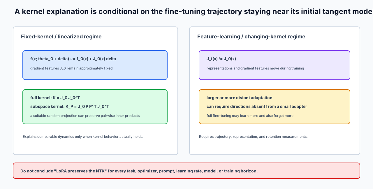
The original NTK paper proves a constant limiting kernel for specific infinite-width networks under its parameterization, initialization, and gradient-flow assumptions. It does not define every finite empirical kernel to be constant. Chizat, Oyallon, and Bach further show that lazy behavior depends on scaling. Yang and Hu construct different infinite-width parameterizations that retain feature learning. Width alone is therefore not the contract; parameterization and update scaling are part of it.

0x09C Restricting Coordinates Produces A Metric, Not Automatically A Projector

Suppose full parameters are restricted through fixed coordinates:

$$\theta = \theta_0+Pu, \qquad P\in\mathbb{R}^{P\times d}$$

The Jacobian with respect to $u$ is:

$$J_u = J_0P$$

Euclidean gradient flow in $u$ induces:

$$K_P = J_0PP^{\top}J_0^{\top}$$

If $P^{\top}P=I_d$, then $PP^{\top}$ is the orthogonal projector onto the chosen parameter subspace. If columns are merely scaled, structured, or non-orthogonal, $PP^{\top}$ also contains that coordinate metric. Calling every such object “the projected full kernel” hides a consequential design choice.

For scalar output rows $j_i^{\top}$ of $J_0$:

$$(K_P)_{ij} = \langle P^{\top}j_i,P^{\top}j_j\rangle$$

A Johnson—Lindenstrauss argument can preserve these pairwise inner products for a finite set of gradient features with high probability when the normalized random projection is sufficiently wide. The rank depends logarithmically on the number of protected pairs and inversely on the requested error. This is a probabilistic finite-dataset statement. It does not guarantee preservation for all inputs, all checkpoints, or a factor map that later changes.

0x09D Derive The Two LoRA Factor Jacobians

Consume M6.3’s orientation:

$$W_{\mathrm{eff}} = W_0+sBA, \qquad B\in\mathbb{R}^{m\times r}, \quad A\in\mathbb{R}^{r\times n}$$

For a batch matrix $X\in\mathbb{R}^{n\times N}$, isolate one linear layer:

$$Y = (W_0+sBA)X \in\mathbb{R}^{m\times N}$$

With column-major vectorization, use the identity $\operatorname{vec}(LZR)=(R^{\top}\otimes L)\operatorname{vec}(Z)$:

$$\operatorname{vec}(BAX) = \big((AX)^{\top}\otimes I_m\big)\operatorname{vec}(B)$$

and also:

$$\operatorname{vec}(BAX) = \big(X^{\top}\otimes B\big)\operatorname{vec}(A)$$

Therefore:

$$J_B = s\big(X^{\top}A^{\top}\otimes I_m\big) \in\mathbb{R}^{mN\times mr}$$ $$J_A = s\big(X^{\top}\otimes B\big) \in\mathbb{R}^{mN\times rn}$$

The concatenated factor Jacobian and its plain-SGD empirical kernel are:

$$J_{\mathrm{LoRA}} = \begin{bmatrix}J_B&J_A\end{bmatrix}$$ $$K_{\mathrm{LoRA}} = J_BJ_B^{\top}+J_AJ_A^{\top}$$

Expanding the Kronecker products gives:

$$K_{\mathrm{LoRA}} = s^2 \left[ \big(X^{\top}A^{\top}AX\big)\otimes I_m + \big(X^{\top}X\big)\otimes BB^{\top} \right]$$

For full-weight coordinates:

$$J_W = X^{\top}\otimes I_m, \qquad K_W = \big(X^{\top}X\big)\otimes I_m$$

At the usual $B_0=0$ start, $J_{A,0}=0$. Only the random $A_0$ path contributes:

$$K_{\mathrm{LoRA},0} = s^2 \big(X^{\top}A_0^{\top}A_0X\big)\otimes I_m$$

This is the tensor-level form of the random-projection explanation. In a deep network, the layer’s upstream output sensitivities multiply this input Gram term. Malladi et al.’s Appendix D writes the resulting layer kernel as the Hadamard product of an output-sensitivity Gram and the projected input Gram. Their theorem then applies a finite-set random-projection bound under a named SGD and kernel-behavior contract.

0x09E Initialization-Time Preservation Is Not Trajectory Preservation

The exact fixture chooses:

$$m=n=r=N=2, \qquad X=I_2, \qquad s=1, \qquad A_0=I_2, \qquad B_0=0$$

This deliberately uses full rank so the initialization algebra is transparent; it is not a compression result. Under the declared parameter order $[\operatorname{vec}(B);\operatorname{vec}(A)]$:

$$J_0 = \begin{bmatrix}I_4&0\end{bmatrix}$$

and:

$$K_{\mathrm{LoRA},0} = I_4 = K_W$$

Use target:

$$T = \begin{bmatrix} 1&1\\ 0&2 \end{bmatrix}$$

and loss $\mathcal L=\frac12\lVert Y-T\rVert_F^2$. With simultaneous plain SGD and $\eta=1/4$:

$$\nabla_B\mathcal L\big|_0 = -T, \qquad \nabla_A\mathcal L\big|_0 = 0$$

so:

$$B_1 = \frac14T = \begin{bmatrix} 1/4&1/4\\ 0&1/2 \end{bmatrix}, \qquad A_1=I_2$$

The first output step is exactly tangent because $A$ did not move. But now:

$$J_{A,1} = I_2\otimes B_1 \neq0$$

and the kernel becomes two copies of:

$$\begin{bmatrix} 9/8&1/8\\ 1/8&5/4 \end{bmatrix}$$

The fixture reports:

relative Jacobian drift squared = 3/16
relative kernel drift squared   = 7/128
kernel alignment squared        = 361/366

High alignment does not mean equality, and exact first-step linearization does not imply fixed features.

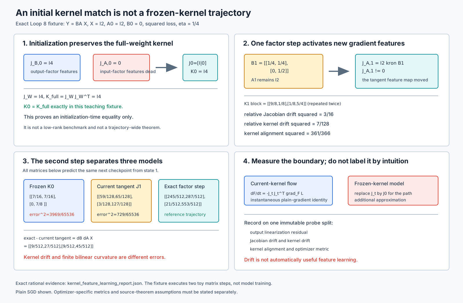
0x09F The Second Step Separates Current Tangent, Frozen Kernel, And Exact Factors

At state one, the old-state gradients are:

$$\nabla_B\mathcal L = \begin{bmatrix} -3/4&-3/4\\ 0&-3/2 \end{bmatrix}$$ $$\nabla_A\mathcal L = \begin{bmatrix} -3/16&-3/16\\ -3/16&-15/16 \end{bmatrix}$$

For simultaneous changes $dB,dA$, the exact finite update is:

$$(B+dB)(A+dA)X = BAX+dBAX+BdAX+dBdAX$$

The current-tangent model includes the middle two terms. The last term is finite bilinear curvature. The frozen-kernel model additionally replaces $J_1$ by $J_0$. The three state-two outputs are:

$$Y_{2,\mathrm{frozen}} = \begin{bmatrix} 7/16&7/16\\ 0&7/8 \end{bmatrix}$$ $$Y_{2,\mathrm{tangent\ at\ }1} = \begin{bmatrix} 59/128&65/128\\ 3/128&127/128 \end{bmatrix}$$ $$Y_{2,\mathrm{exact}} = \begin{bmatrix} 245/512&287/512\\ 21/512&553/512 \end{bmatrix}$$

Their exact difference exposes the finite factor cross term:

$$Y_{2,\mathrm{exact}} - Y_{2,\mathrm{tangent\ at\ }1} = \begin{bmatrix} 9/512&27/512\\ 9/512&45/512 \end{bmatrix}$$

The squared errors are:

$$\left\lVert Y_{2,\mathrm{exact}}-Y_{2,\mathrm{tangent\ at\ }1} \right\rVert_F^2 = \frac{729}{65536}$$ $$\left\lVert Y_{2,\mathrm{exact}}-Y_{2,\mathrm{frozen}} \right\rVert_F^2 = \frac{3969}{65536}$$

The frozen-kernel discrepancy is larger because it combines feature drift with finite bilinear curvature. Reporting only one aggregate error cannot identify which approximation failed.

0x09G A Smaller Rank Can Delete Probe Directions

Now set $r=1$, $A_0=[1\;0]$, and $B_0=0$ on the same $X=I_2$ fixture. Then:

$$J_{\mathrm{LoRA},0} = \begin{bmatrix} 1&0&0&0\\ 0&1&0&0\\ 0&0&0&0\\ 0&0&0&0 \end{bmatrix}$$

so:

$$K_{\mathrm{LoRA},0} = \operatorname{diag}(1,1,0,0), \qquad K_W=I_4$$

The projected kernel has rank two while the full kernel has rank four, with squared Frobenius discrepancy two. This deterministic case does not contradict the random-projection theorem. It shows why the theorem needs randomness, normalization, a sufficiently large projection dimension, a finite protected set, and a probability statement.

0x09H The Optimizer Changes The Kernel Analog

For plain SGD, the tangent metric is:

$$K_{\mathrm{SGD}} = JJ^{\top}$$

For a fixed preconditioner, it is $JMJ^{\top}$. Adaptive moments make $M_t$ depend on coordinate history, data order, clipping, epsilon, and decay. There need not be one fixed symmetric matrix that describes the full trajectory.

Malladi et al. analyze an early-stage SignGD approximation to Adam and define an asymmetric kernel analog:

$$K_{\mathrm{A\text{-}Sign}}(x,x') = \left\langle \nabla_\theta f(x;\theta_0), \operatorname{sign}\big(\nabla_\theta f(x';\theta_0)\big) \right\rangle$$

For the exact probe:

$$J = \begin{bmatrix} 1&2\\ 3&4 \end{bmatrix}$$

the three candidate objects are:

$$JJ^{\top} = \begin{bmatrix} 5&11\\ 11&25 \end{bmatrix}$$ $$J\operatorname{sign}(J)^{\top} = \begin{bmatrix} 3&3\\ 7&7 \end{bmatrix}$$ $$\operatorname{sign}(J)\operatorname{sign}(J)^{\top} = \begin{bmatrix} 2&2\\ 2&2 \end{bmatrix}$$

The asymmetric analog is visibly not $JJ^{\top}$ and not symmetric. The source paper also studies a symmetric sign-feature variant for kernel regression. Neither object licenses replacing a general late-stage AdamW run with the plain-SGD NTK.

0x09I What The Source Experiment Actually Shows

Malladi et al. compare a pretrained model, its initial linearization, and the actual fine-tuned model across their task and prompt protocols. The gap varies substantially across tasks and between SGD and Adam. That is evidence that kernel behavior must be measured under the protocol rather than presumed from model size.

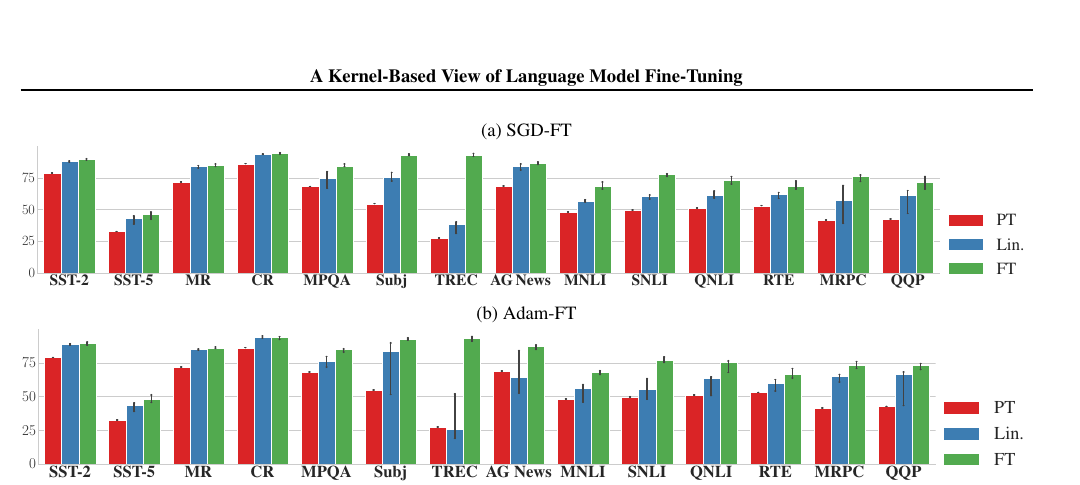
The image is a crop of Figure 2 from A Kernel-Based View of Language Model Fine-Tuning, reproduced without redrawing under CC BY 4.0. It reports the authors’ experiments on their selected tasks, prompts, optimizers, splits, and hyperparameters. It is not a result of the exact fixture and not a universal comparison between LoRA and full fine-tuning.

The paper’s LoRA preservation argument has an explicit implication order:

full fine-tuning exhibits kernel behavior under the named protocol
    plus
the normalized random LoRA projection preserves finite-set gradient inner products
    implies
the LoRA kernel analog is close on that protected set

Reversing that implication is invalid. A close initialization kernel does not prove that the nonlinear full-fine-tuning or LoRA trajectory stays in the kernel regime.

0x09J Diagnostics Must Separate Three Residuals

On an immutable probe split, record at every diagnostic checkpoint:

$$R_{\mathrm{lin}}(t) = \frac{ \left\lVert F_t-F_0-J_0(\theta_t-\theta_0) \right\rVert_2 }{ \max\big(\lVert F_t-F_0\rVert_2,\epsilon\big) }$$ $$D_J(t) = \frac{\lVert J_t-J_0\rVert_F}{\max(\lVert J_0\rVert_F,\epsilon)}$$ $$D_K(t) = \frac{\lVert K_t-K_0\rVert_F}{\max(\lVert K_0\rVert_F,\epsilon)}$$

and a scale-insensitive kernel alignment:

$$A_K(t) = \frac{ \langle K_t,K_0\rangle_F }{ \max\big(\lVert K_t\rVert_F\lVert K_0\rVert_F,\epsilon\big) }$$

These answer different questions:

Diagnostic	Detects	Does not prove
$R_{\mathrm{lin}}$	failure of the initialization Taylor model on selected outputs	that the kernel itself is stable
$D_J$	coordinate-level gradient-feature drift	useful learned representations; it is gauge and parameterization sensitive
$D_K$	drift of the chosen tangent metric on the probe split	low drift off the probe split or under another optimizer metric
$A_K$	directional agreement after discarding overall scale	equal convergence rate or equal kernel magnitude
task and retention metrics	operational learning and forgetting	mechanism without the trajectory diagnostics

Parameter distance alone is insufficient. Loop 7 showed that an exact factor gauge can make $A$ and $B$ arbitrarily large or small while preserving $BA$; conversely, a modest parameter move can materially change selected function outputs.

0x09K Do Not Materialize A Production-Scale Kernel

For large models, use Jacobian-vector and vector-Jacobian products. For random output probes $z_q$:

$$K_tz_q = J_t\big(J_t^{\top}z_q\big)$$

and estimate kernel-difference energy with:

$$\lVert K_t-K_0\rVert_F^2 \approx \frac1Q \sum_{q=1}^{Q} \left\lVert (K_t-K_0)z_q \right\rVert_2^2$$

The probe distribution, count $Q$, seed, output stacking, dtype, and estimator uncertainty are part of the result.

probe = freeze_probe_split(
    examples=probe_examples,
    output_selector=selected_logits,
    dropout=False,
    order="example_then_output",
)

theta0 = load_adapter_initial_state()
F0 = forward(theta0, probe)

for checkpoint in checkpoints:
    theta_t = load(checkpoint)
    Ft = forward(theta_t, probe)
    F_linear = F0 + jvp_at(theta0, theta_t - theta0, probe)

    for z in fixed_random_output_probes:
        K0_z = jvp_at(theta0, vjp_at(theta0, z, probe), probe)
        Kt_z = jvp_at(theta_t, vjp_at(theta_t, z, probe), probe)
        accumulate_kernel_drift(Kt_z - K0_z)

    record(
        output_linearization_residual=relative_error(Ft, F_linear, F0),
        kernel_drift_estimate=finalize_probe_estimator(),
        optimizer=optimizer_state_contract(checkpoint),
        task_metrics=evaluate_target(checkpoint),
        retention_metrics=evaluate_retention(checkpoint),
    )

If the optimizer metric is $M_t$, compute $J_tM_tJ_t^{\top}z$ instead of silently using $J_tJ_t^{\top}z$. For AdamW this requires a declared approximation to moment state and decoupled decay; there is no automatic fixed-kernel shortcut.

0x09L Training And Runtime Integration

A defensible experiment runs at least three matched paths:

1. the nonlinear LoRA model with both factors trainable;
2. the initialization-linearized LoRA model under the same declared optimizer analog;
3. a fixed-random-feature path that freezes the initially nonzero factor.

Optionally add full fine-tuning, but match data order, tokens, batch construction, checkpoint selection, output definition, and evaluation cadence. “Same learning rate” is not automatically a fair comparison when parameter coordinates and optimizer metrics differ.

Checkpoint state must include:

base checkpoint and tokenizer identity
adapter factor tensors, scale, orientation, and target modules
optimizer moments, step counters, clipping, decay, and scheduler
probe-split identity and selected output coordinates
dropout/eval state and numeric precision
JVP/VJP estimator seeds and probe vectors
linearization base point and checkpoint distance
target, validation, and retention measurements

Kernel diagnostics are offline evidence. They do not change the merge or serving ABI owned by M6.3 and M6.5. A deployment still serves the nonlinear adapter unless a separate release explicitly packages a linearized surrogate.

0x09M Design Alternatives Expose Different Assumptions

Design	Moving features?	Kernel object	What it isolates	Main limitation
initialization linearization	no	$J_0J_0^{\top}$ or declared optimizer metric	frozen-kernel prediction	omits feature drift and finite curvature
freeze $A_0$, train $B$	no factor-feature change in this linear-layer path	projected random-feature kernel	random projection adequacy	cannot rotate the input factor
train both $A,B$	yes after the zero factor moves	$K(A_t,B_t)$	bilinear feature adaptation	kernel and factor gauge evolve
fixed orthonormal subspace $P$	no	$J_0PP^{\top}J_0^{\top}$	global coordinate restriction	not layer-local low-rank geometry
plain full fine-tuning	model dependent	full empirical NTK	unrestricted tangent features	highest trainable state and forgetting risk
fixed preconditioned flow	maybe	$J_tMJ_t^{\top}$	optimizer metric sensitivity	fixed $M$ does not model adaptive history
SignGD analog	source-contract dependent	asymmetric sign kernel	early normalized-gradient behavior	not a general AdamW trajectory theorem
feature-learning parameterization	yes by construction in the cited limit	evolving/data-adapted features	rich-regime alternative	theorem assumptions differ from finite LoRA

0x09N Paper-By-Contract Comparison

Source	Frozen object	Main result consumed here	Required boundary
Jacot, Gabriel, and Hongler	limiting NTK under their infinite-width setup	function-space kernel gradient and constant limiting kernel	finite LoRA empirical kernels need not be constant
Chizat, Oyallon, and Bach	initialization linearization under lazy scaling	lazy behavior is scaling-induced and paths can be bounded near linearization	laziness is not synonymous with overparameterization alone
Yang and Hu	parameterization-dependent infinite-width limit	feature learning can survive a different infinite-width scaling	not a direct finite-LLM LoRA guarantee
Malladi et al.	optimizer-specific initialization kernel analog	kernel-behavior definition, LoRA projected-kernel formula, finite-set preservation, task evidence	meaningful only when the underlying fine-tuning protocol exhibits kernel behavior
Jang, Lee, and Ryu	an NTK-regime affine prediction problem	low-rank solution and landscape theorems	owned by 0x0A; not evidence that a practical run remains in the NTK regime

0x09O Kernel-Regime Failure Lab

Failure	Hidden collapse	Observable consequence
$\dot F=-K_tg$ quoted as fixed-kernel proof	current kernel vs $K_0$	an exact chain-rule identity is misread as a lazy-training theorem
initial kernel equality treated as trajectory equality	initialization vs path	activated $J_A$ columns and later drift are ignored
first-step Taylor equality treated as long-run linearization	one zero gradient vs persistent fixed features	second-step bilinear cross term appears unexplained
$PP^{\top}$ called a projector without $P^{\top}P=I$	subspace vs coordinate metric	scaling changes the apparent kernel
random projection theorem applied to deterministic rank one	probabilistic finite-set guarantee omitted	protected directions disappear
layer-local input Gram treated as the whole network kernel	local Jacobian vs upstream sensitivity	output-gradient geometry is absent
$JJ^{\top}$ used for AdamW	plain SGD metric vs adaptive history	kernel prediction follows the wrong update direction
low $D_J$ alone called kernel behavior	fixed features vs output linearization	nonlinear remainder can still be large
high kernel alignment called equality	angle vs magnitude	learning rates and convergence times disagree
Jacobian drift called beneficial feature learning	motion vs utility	features move while target and retention quality worsen
parameter distance used without gauge normalization	factor coordinates vs function	exact refactorization looks like large learning
probe split reused for model selection without disclosure	diagnostic vs selection data	optimistic kernel-fit evidence
source Figure 2 treated as a LoRA benchmark	full-fine-tuning source protocol vs local fixture	unrelated methods and tasks are conflated

0x09P Loop 8 Handoff

Loop 8 establishes what a kernel explanation can and cannot claim. Loop 9 may now study expressive-power and NTK-regime optimization theorems, but it must consume this boundary: a theorem stated inside an NTK model does not prove that an observed nonlinear training run entered or remained inside that model.

0x0A Expressive Power, Optimization Geometry, And Deep Composition

The phrase “rank $r$ is enough” is incomplete. Enough to represent one matrix? Enough for a constructive deep-network existence theorem? Enough to remove spurious second-order stationary points in a perturbed linearized objective? Enough to compress one gradient-descent trajectory?

Those are different questions with different mathematical objects. Loop 8 already established another boundary: a theorem inside an NTK model does not prove that an observed nonlinear run entered or stayed in that model. This section consumes that boundary rather than silently discarding it.

0x0AA Owner Contract: Carry The Quantifiers With The Rank

Every claim in this section must declare six coordinates:

Coordinate	Question that must be answered
Object	One matrix, a product of matrices, a ReLU FNN, a Transformer, a linearized empirical loss, or a training trajectory?
Quantifier	Does the result say “there exists,” “for every target,” “with probability one,” or “almost every perturbation”?
Architecture	Width, depth, residual path, weight shapes, biases, target modules, and nonlinearities?
Optimization	No optimizer, gradient descent, second-order stationary points, or an optimizer-specific trajectory?
Rank statement	Necessary, sufficient, an upper bound, an approximation tail, or a configured factor width?
Exclusion	Which practical conclusion is not proved?

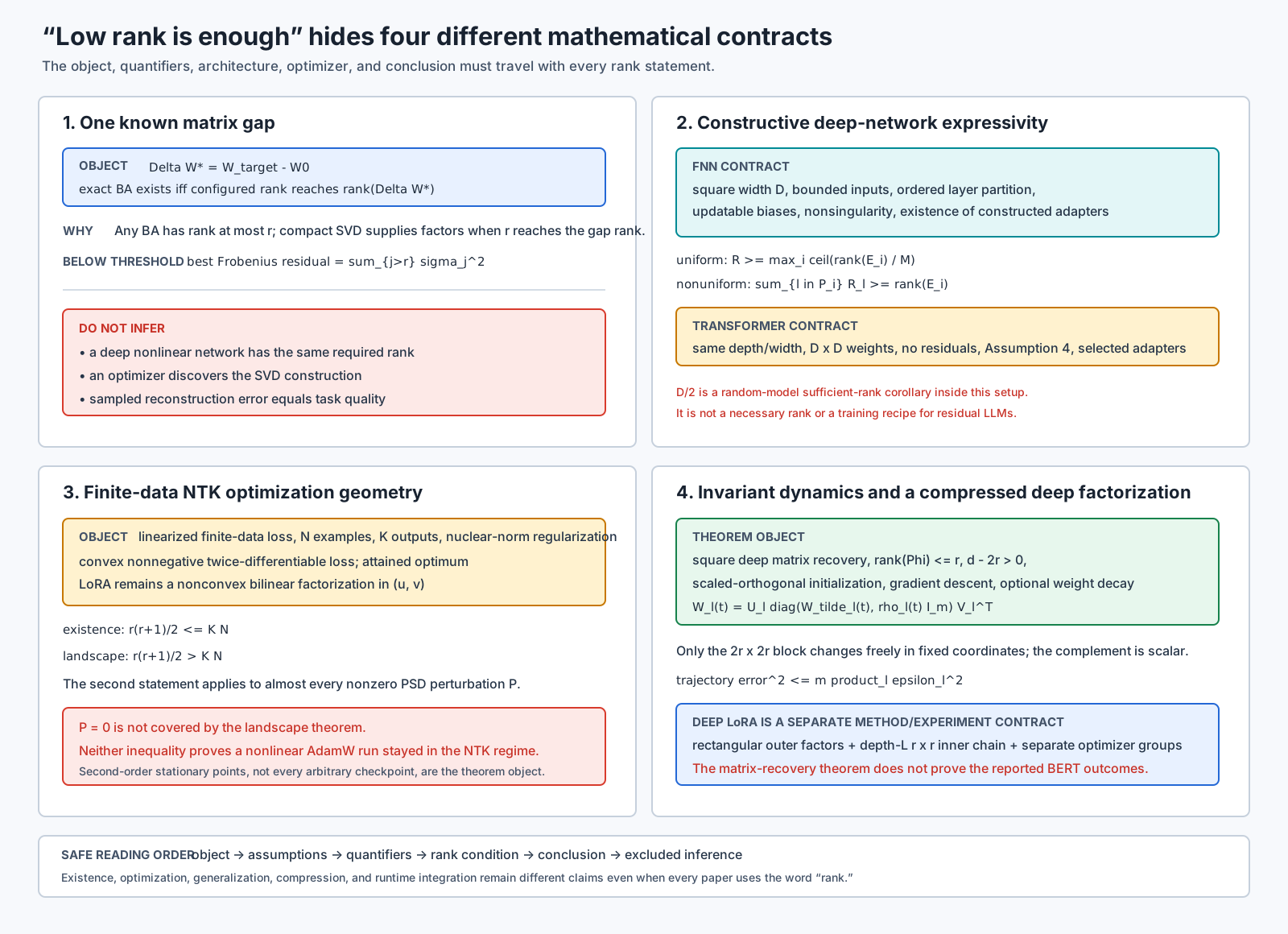
The section owns theorem assumptions, proof structure, exact finite counterexamples, and diagnostics. It does not reopen M6.3’s vanilla operator, M6.4’s variant catalog, M6.5’s multi-tenant serving state, or M6.9’s routed composition system.

0x0AB One Known Matrix: Exact Rank Is Necessary And Sufficient

Freeze one matrix $W_0\in\mathbb{R}^{m\times n}$ and one target matrix $W_*$. Their additive functionality gap is

$$E=W_*-W_0.$$

An adapter with configured rank $r$ writes

$$\Delta W=BA, \qquad B\in\mathbb{R}^{m\times r}, \quad A\in\mathbb{R}^{r\times n}.$$

Necessity is one line:

$$\operatorname{rank}(BA)\leq r.$$

If $BA=E$, then necessarily

$$r\geq\operatorname{rank}(E).$$

Sufficiency comes from the compact SVD. If

$$E=U_q\Sigma_qV_q^{\top}, \qquad q=\operatorname{rank}(E),$$

then for any $r\geq q$ one valid padded factorization is

$$B= \begin{bmatrix} U_q\Sigma_q^{1/2}&0 \end{bmatrix}, \qquad A= \begin{bmatrix} \Sigma_q^{1/2}V_q^{\top}\\ 0 \end{bmatrix}.$$

Therefore, for one known additive matrix gap,

$$\min\{r:\exists A,B,\ BA=E\}=\operatorname{rank}(E).$$

Below that threshold, Eckart—Young gives a different statement:

$$\min_{\operatorname{rank}(X)\leq r}\|E-X\|_F^2 = \sum_{j>r}\sigma_j(E)^2.$$

That is an optimal post-hoc matrix approximation. It does not say factor training finds the truncation, nor that a small weight residual preserves task behavior. Loop 5 owns those reconstruction and output-weighted distinctions.

Exact $3\times3$ Trace

The Loop 9 fixture freezes

$$W_0=I_3, \qquad W_*=\operatorname{diag}(5,3,1),$$

so

$$E=\operatorname{diag}(4,2,0), \qquad \operatorname{rank}(E)=2.$$

A rank-two factorization is

$$B= \begin{bmatrix} 4&0\\ 0&2\\ 0&0 \end{bmatrix}, \qquad A= \begin{bmatrix} 1&0&0\\ 0&1&0 \end{bmatrix},$$

and $BA=E$ exactly. The residual ledger is

Configured rank	Best squared Frobenius residual
$0$	$4^2+2^2=20$
$1$	$2^2=4$
$2$	$0$

No deep-network rank has been inferred. The fixture has proved only what it computed.

0x0AC A Product Of Adapted Matrices Has A Telescoping Rank Budget

Depth changes the object. Let the frozen linear map be

$$F_0=W_LW_{L-1}\cdots W_1$$

and the adapted map be

$$F_{\Delta} = (W_L+\Delta W_L)\cdots(W_1+\Delta W_1).$$

Do not expand all $2^L-1$ interaction terms. Insert and subtract one partially adapted product at a time:

$$F_{\Delta}-F_0 = \sum_{\ell=1}^{L} \left(\prod_{i=\ell+1}^{L}W_i\right) \Delta W_{\ell} \left(\prod_{i=1}^{\ell-1}(W_i+\Delta W_i)\right).$$

Each summand has rank at most $\operatorname{rank}(\Delta W_\ell)$. Therefore,

$$\operatorname{rank}(F_{\Delta}-F_0) \leq \sum_{\ell=1}^{L}\operatorname{rank}(\Delta W_\ell) \leq LR$$

when every layer uses rank at most $R$.

This derivation supplies a necessary rank budget for the product gap. It does not yet establish that every rank-at-most-$LR$ gap can be allocated to valid layer updates. The constructive reverse direction needs the invertibility conditions in Zeng and Lee’s product lemma: left and right context products must remain invertible while the low-rank pieces are assigned sequentially.

Why Allocation Matters

Take two frozen identity layers and target product

$$F_*=\operatorname{diag}(2,3,1).$$

One allocation puts the complete gap in the first layer:

$$W_1'=\operatorname{diag}(2,3,1), \qquad W_2'=I_3,$$

with update ranks $[2,0]$. Another distributes the gap:

$$W_1'=\operatorname{diag}(2,1,1), \qquad W_2'=\operatorname{diag}(1,3,1),$$

with update ranks $[1,1]$. Both satisfy

$$W_2'W_1'=\operatorname{diag}(2,3,1).$$

For the distributed case, the telescoping terms are

$$W_2\Delta W_1 = \operatorname{diag}(1,0,0),$$

and

$$\Delta W_2(W_1+\Delta W_1) = \operatorname{diag}(0,2,0).$$

Their sum is the rank-two product gap. Depth reduced the maximum per-layer update rank from two to one without changing the end-to-end function.

This does not make rank additive in general. Loop 6 already showed that low-rank sums can align, cancel, or grow. Here the point is narrower: one end-to-end function can admit multiple layerwise allocations.

0x0AD From Product Algebra To ReLU FNN Expressivity

Zeng and Lee study whether adapters exist. Their paper explicitly excludes optimization and generalization from the expressive-power question.

Use separate notation for the two depths:

target FNN:
    depth L_target
    square width-D weights W_bar_i

frozen/adapted FNN:
    depth L_frozen >= L_target
    square width-D weights W_l + Delta W_l

The input domain is bounded, biases may be changed, and an ordered partition

$$\mathcal{P}=\{P_1,\ldots,P_{L_{target}}\}$$

assigns consecutive frozen layers to each target layer. For one partition block, define its matrix functionality gap

$$E_i = \overline W_i - \prod_{\ell\in P_i}W_{\ell}.$$

Why Bias Updates Appear

A product lemma alone is linear. To make a block of ReLU layers implement one target ReLU layer, the construction uses biases in the earlier layers of the block to keep their preactivations positive over the bounded input set. Those ReLUs then act linearly. The final layer in the block restores the target preactivation and target bias before the remaining ReLU.

So the proof does not say arbitrary intermediate ReLUs disappear during ordinary training. It constructs biases that linearize selected intermediate layers over the theorem’s bounded domain.

This yields an immediate scope requirement:

theorem construction allows bias updates
!=
bias-frozen LoRA implementation

If a practical setup freezes all biases, this proof cannot be imported unchanged.

0x0AE Uniform Partition And Uniform Rank

For a uniform partition, let

$$M=\left\lfloor\frac{L_{frozen}}{L_{target}}\right\rfloor$$

be the number of adapted layers assigned to each target layer. The telescoping argument gives each block an aggregate rank budget $MR$. Under the paper’s Assumption 1, a sufficient exact-recovery condition is

$$R \geq \left\lceil \frac{ \max_i\operatorname{rank}(E_i) }{M} \right\rceil.$$

The denominator $M$ is not magic. It comes from distributing a partition gap across $M$ rank-$R$ layer updates:

$$\sum_{\ell\in P_i}\operatorname{rank}(\Delta W_\ell) \leq MR.$$

The nonsingularity assumption is what makes the constructive sequential allocation feasible. For independently sampled continuous random weights, the paper proves its assumption holds with probability one and derives the generic sufficient threshold

$$R\geq\frac{D}{M}.$$

“With probability one” applies to the random matrix model in the corollary. It is not a frequency claim about pretrained checkpoints, and $D/M$ is not a recommended sweep endpoint.

0x0AF General Partitions And Nonuniform Ranks

Uniform allocation can waste rank. If the first target layer already matches its assigned frozen block, its gap rank is zero. Giving that block the same rank as a difficult block spends parameters without improving the theorem’s coverage.

The nonuniform theorem assigns rank $R_\ell$ per adapted layer and requires, for every partition block,

$$\sum_{\ell\in P_i}R_\ell \geq \operatorname{rank}(E_i).$$

This is a partition coverage condition. It is not a claim that only the scalar sum matters during training. Location, conditioning, activation patterns, and optimizer state can still make two equal-budget allocations behave differently.

The theorem also separates two design choices that benchmarks often collapse:

Choice	Changed object
Partition $\mathcal P$	Which frozen depth composes to approximate each target layer
Rank vector $(R_1,\ldots,R_L)$	How much rank budget each adapted matrix receives

M6.4 owns named adaptive-rank algorithms. M6.7 owns the theoretical reason nonuniform allocation can matter.

0x0AG Below Exact Recovery: Propagated Singular Tails

When a partition does not have enough aggregate rank, define

$$\varepsilon_i = \sigma_{\sum_{\ell\in P_i}R_\ell+1}(E_i).$$

This is the first omitted singular value of the $i$-th partition gap, not the task loss. Zeng and Lee’s approximation theorem propagates these local approximation terms through the target network. In structural form,

$$\mathbb{E}\|\widehat f(x)-f(x)\|_2^2 \leq \beta \sum_{i=1}^{L_{target}} \left( \max_k\|\overline W_k\|_F+\varepsilon_k \right)^{L_{target}-i} \varepsilon_i,$$

where $\beta$ collects the paper’s input-covariance and target-weight/bias magnitude terms.

The shape of the bound matters:

1. a discarded singular tail enters locally;
2. later target layers can amplify that local error;
3. input covariance and parameter magnitudes are part of the contract;
4. the result is an existence bound for constructed adapters.

A small $\varepsilon_i$ alone is not enough to claim a small final function error. A small theorem bound still does not establish optimizer reachability or held-out task quality.

0x0AH Transformer Expressivity: Reconstruct The Architecture Before The Headline

The paper’s Transformer result is not stated for an ordinary residual LLM block. Its formal setup freezes these coordinates:

target and frozen network:
    same number L of Transformer blocks
    same embedding dimension D
    every weight matrix represented as D x D
    multi-head self-attention followed by tokenwise FFN
    skip connections excluded for analytical feasibility

adaptation:
    attention K/Q/V/O adapters
    final block's second FFN matrix adapter
    output-matrix adapter
    updated bias vectors
    other low-rank adapters set to zero in the construction

The no-residual choice is not cosmetic. Residual addition changes the block function and the algebra by which an adapted block is matched to a target block.

Why The Rank Bound Contains A Division By Two

Attention exposes matrix products, not isolated weights. Score logits depend on a product like

$$W_K^{\top}W_Q.$$

Adapting both factors changes that product by

$$(W_K+\Delta W_K)^{\top}(W_Q+\Delta W_Q)-W_K^{\top}W_Q$$ $$= W_K^{\top}\Delta W_Q + \Delta W_K^{\top}(W_Q+\Delta W_Q).$$

Each term has rank at most $R$, so the product gap has rank at most $2R$. The value/output path has the same structure through products involving $W_O$ and $W_V$, with FFN bridge matrices entering after the first block.

The paper defines a block functionality-gap rank $G_i$ from these score and value-path product gaps, and an output-layer gap $G_{L+1}$. Under Assumption 4, its sufficient condition is

$$R \geq \max_{i\in[L+1]} \left\lceil\frac{G_i}{2}\right\rceil.$$

The proof aligns attention scores before softmax, aligns the first FFN output before ReLU, and then chooses the output path to finish the equality. Under that construction,

$$\widehat f(X)=f(X) \qquad \text{for every }X\in\mathbb{R}^{D\times N}.$$

For independently drawn continuous random weights, the paper’s corollary yields the headline sufficient rank $D/2$. The full statement is therefore:

D/2 is sufficient with probability one
for the paper's random same-size, D x D, no-residual Transformer model,
under its nonsingularity assumption and constructive adapter/bias placement.

It does not say:

rank D/2 is necessary for pretrained residual LLMs
rank D/2 is the best benchmark rank
gradient training will find the constructed adapters
smaller ranks cannot solve structured downstream tasks

0x0AI Expressivity Does Not Imply Trainability

An existence proof answers

$$\exists(A,B):\widehat f_{A,B}=f_*.$$

Training asks whether a declared optimizer, initialization, data order, regularizer, and finite precision trajectory reaches a useful solution. Those questions are not logically equivalent:

$$\text{representable} \nRightarrow \text{reachable by the chosen optimizer}.$$

The constructive adapters can depend on target weights that are not available in downstream fine-tuning. That is acceptable for an expressivity theorem and unusable as a direct training algorithm unless those objects can be estimated.

This is where the NTK paper enters. It does not strengthen the same theorem. It changes the object from a deep-network function class to a finite-data linearized optimization problem.

0x0AJ The NTK Problem Is A Linearized Full-Update Object

Jang, Lee, and Ryu select $T$ pretrained weight matrices

$$W^{(i)}_0\in\mathbb{R}^{m_i\times n_i}, \qquad i=1,\ldots,T,$$

and stack their updates into one matrix variable

$$\delta=uv^{\top}, \qquad u\in\mathbb{R}^{m\times r}, \quad v\in\mathbb{R}^{n\times r},$$

where $m=\sum_i m_i$ and $n=\sum_i n_i$. The Jacobian feature object $G(X)$ is block diagonal across the selected matrices.

For $N$ examples and $K$ output coordinates, the nonlinear network is replaced by its first-order model:

$$f_{W_0+\delta}(X_i) \approx f_{W_0}(X_i) + \langle G(X_i),\delta\rangle.$$

The loss is assumed convex, nonnegative, and twice differentiable in the model output. Cross entropy and mean squared error fit that loss-side assumption; the network linearization remains a separate regime assumption.

The empirical linearized loss is

$$\widehat{\mathcal L}(\delta) = \frac{1}{N} \sum_{i=1}^{N} \ell\left( f_{W_0}(X_i)+\langle G(X_i),\delta\rangle, Y_i \right).$$

This function is convex in the full matrix $\delta$ but nonconvex in the factors $(u,v)$.

0x0AK Why Factor Weight Decay Becomes A Nuclear Norm

The factor identity

$$\|\delta\|_* = \frac{1}{2} \min_{uv^{\top}=\delta} \left( \|u\|_F^2+\|v\|_F^2 \right)$$

connects factor weight decay to the nuclear-norm-regularized full-update problem

$$\widehat{\mathcal L}_{\lambda}(\delta) = \widehat{\mathcal L}(\delta) + \lambda\|\delta\|_*.$$

This identity requires a compatible regularizer on both factors. It does not mean arbitrary decoupled AdamW, per-factor learning rates, clipping, or exclusion rules optimize the same matrix objective. Loop 7 already showed that factor-coordinate optimizer choices change product dynamics.

0x0AL Low-Rank Existence Comes From A PSD Lift And Dimension Counting

Introduce

$$Q= \begin{bmatrix} u\\v \end{bmatrix}, \qquad Z=QQ^{\top}\succeq0.$$

The update $\delta=uv^{\top}$ is an off-diagonal block of $Z$. The lifted objective depends on $Z$ through at most $KN$ scalar linearized predictions plus the trace regularizer.

If a rank-$s$ optimum $Z_*$ has a nonzero symmetric direction inside its column space that is invisible to all $KN$ prediction constraints, one can move along that direction while preserving the objective until an eigenvalue reaches zero. The rank falls. Repeat until no such direction remains.

The symmetric matrices supported on an $s$-dimensional range have dimension

$$\dim\mathcal S(Z_*) = \frac{s(s+1)}{2}.$$

The measurement operator has rank at most $KN$. At the terminal low-rank optimum, dimension counting gives

$$\frac{s(s+1)}{2} \leq KN.$$

The theorem therefore says: if the nuclear-norm-regularized linearized full-update problem has a global minimizer, there exists at least one global minimizer whose rank obeys this bound.

It does not say every minimizer is low rank. It does not say the original nonlinear full-fine-tuning update has that rank. It does not say a rank-$s$ factor optimizer reaches that minimizer.

0x0AM The Landscape Theorem Uses The Opposite Strict Inequality

The no-spurious-second-order-stationary-point result requires the configured factor rank $r$ to satisfy

$$\frac{r(r+1)}{2} > KN.$$

This is not a contradiction. The two inequalities answer different questions:

Inequality	Rank variable	Conclusion
$s(s+1)/2\leq KN$	rank of at least one full-update optimum	a low-rank optimum exists
$r(r+1)/2>KN$	configured factor width	generic perturbed factorized landscape has no nonglobal SOSPs

The landscape objective is also perturbed:

$$\widehat{\mathcal L}_{\lambda,P}(u,v) = \widehat{\mathcal L}(uv^{\top}) + \frac{\lambda}{2} \left(\|u\|_F^2+\|v\|_F^2\right) + \langle P,QQ^{\top}\rangle,$$

where $P\succeq0$. For almost every nonzero $P$, all second-order stationary points are global minimizers of this perturbed objective.

Three qualifiers are load-bearing:

1. almost every nonzero perturbation is not deterministic $P=0$;
2. second-order stationary point is not every first-order stationary point or arbitrary stopped checkpoint;
3. linearized loss is not the original nonlinear network objective.

The paper explicitly notes that its theorem does not apply directly to the practical deterministic choice $P=0$. Its corollary instead bounds how far a minimizer of a sufficiently small random perturbation can be from the optimum value of the unperturbed objective.

Exact Triangular-Number Trace

For $N=3$ and $K=2$,

$$KN=6.$$

The largest rank satisfying the existence inequality is $s=3$ because

$$\frac{3(3+1)}{2}=6.$$

The smallest configured rank satisfying the landscape inequality is $r=4$ because

$$\frac{4(4+1)}{2}=10>6.$$

Writing only "$r\sim\sqrt{N}$" erases $K$, the triangular count, strictness, the change of rank variable, and the perturbation.

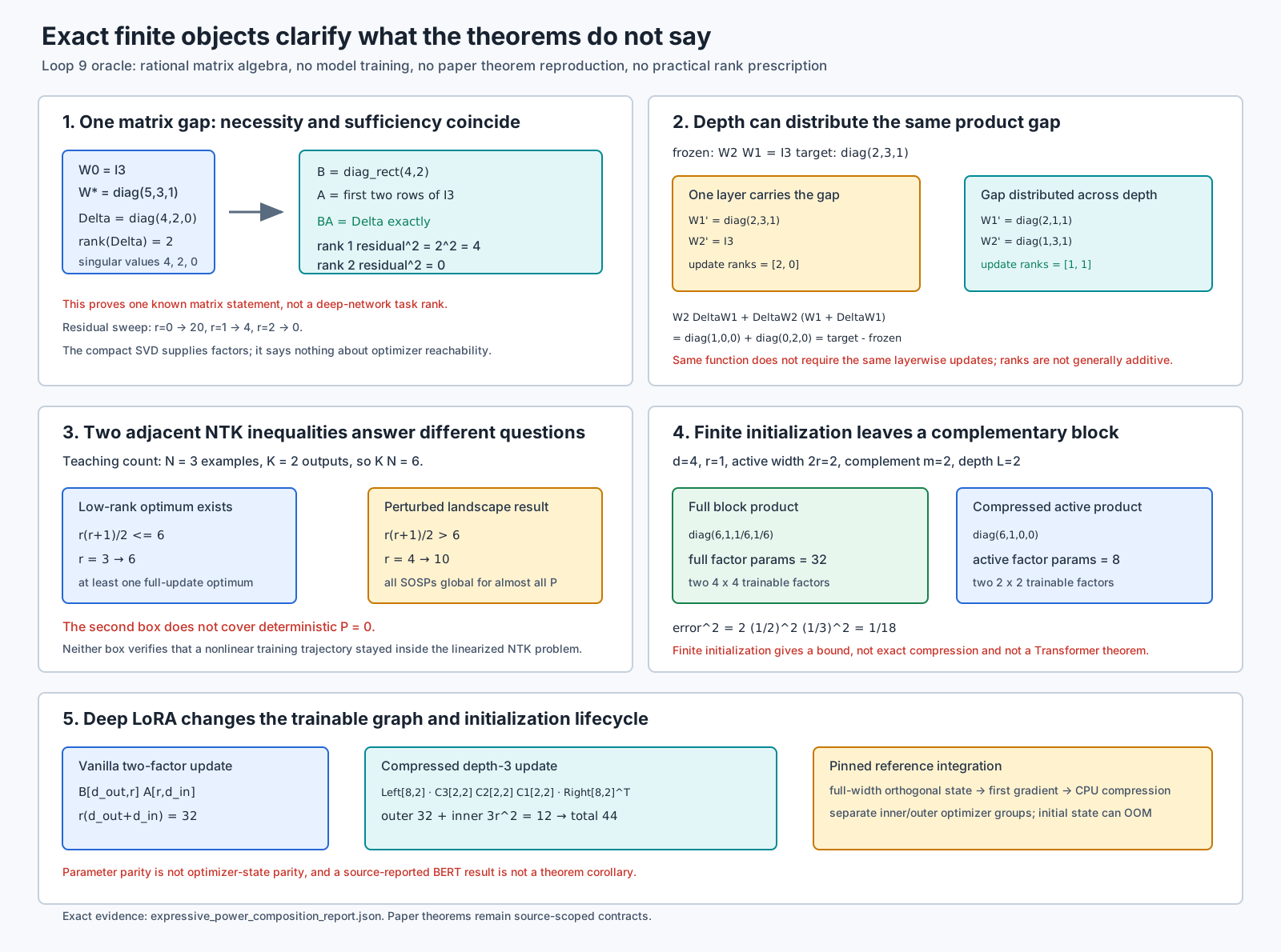
0x0AN Source Geometry: Constraint Count Versus Low-Rank Surface

Jang et al.’s Figure 1 uses a $2\times2$ matrix and a rank-one surface to visualize the existence theorem. As the number of scalar constraints increases from one to three, the affine set of global minima shrinks. At $N=3$ in that toy setup, the global-minimum set no longer intersects the rank-one surface, although a rank-two optimum remains.

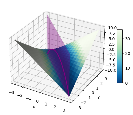
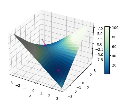
These are the unmodified plot panels extracted from Jang et al., Figure 1, under the PMLR CC BY 4.0 publication agreement. They are source-reported geometric evidence, not a repository reproduction. The surfaces illustrate one theorem’s dimension count; they do not establish an LLM rank rule.

0x0AO What The NTK Experiments Do And Do Not Validate

The source experiment uses a linearized RoBERTa-base model, prompt-based fine-tuning, $N=32$ examples, and $K=2$ labels on six NLP tasks. For that count,

$$\frac{r(r+1)}{2}>64$$

first holds at $r=11$. The paper compares training curves under its declared setup and reports convergence behavior consistent with the analyzed landscape.

That experiment is not a test of nonlinear production LoRA with arbitrary AdamW settings. It does not validate a universal square-root rank rule. A practical nonlinear run needs the Loop 8 diagnostics: linearization residual, Jacobian drift, kernel drift, optimizer metric, and probe-split discipline.

The paper also gives a generalization bound under additional assumptions, including bounded Jacobian-feature norms, an attained nonzero population optimum, a declared regularization choice, and the perturbed-objective setup. “No spurious SOSPs” and “generalizes well” remain separate theorems even inside the same paper.

0x0AP Deep Factorization Changes The Trajectory Object Again

Yaras et al. begin with deep square matrix factorization, not Transformer fine-tuning. Freeze

$$f(\Theta)=W_LW_{L-1}\cdots W_1$$

and solve

$$\min_{\Theta} \frac{1}{2} \|f(\Theta)-\Phi\|_F^2,$$

where

$$W_\ell\in\mathbb{R}^{d\times d}, \qquad \operatorname{rank}(\Phi)\leq r, \qquad d-2r>0.$$

Initialization is scaled orthogonal:

$$W_\ell(0)W_\ell(0)^{\top} = W_\ell(0)^{\top}W_\ell(0) = \epsilon_\ell^2I_d.$$

Gradient descent with optional weight decay follows

$$W_\ell(t+1) = (1-\eta\lambda)W_\ell(t) - \eta\nabla_{W_\ell}\mathcal L(\Theta(t)).$$

These coordinates are part of the theorem. Replacing squared matrix-recovery loss by cross entropy, GD by AdamW, square factors by arbitrary Transformer projections, or scaled-orthogonal initialization by standard LoRA initialization changes the problem.

0x0AQ The Invariant Block Has Width $2r$, Not $r$

Let

$$m=d-2r>0.$$

The source theorem constructs fixed orthogonal matrices $U_\ell,V_\ell$ with $V_{\ell+1}=U_\ell$ such that every iterate has block form

$$W_\ell(t) = U_\ell \begin{bmatrix} \widetilde W_\ell(t)&0\\ 0&\rho_\ell(t)I_m \end{bmatrix} V_\ell^{\top},$$

where

$$\widetilde W_\ell(t)\in\mathbb{R}^{2r\times2r}.$$

The complement does not have arbitrary matrix dynamics. It remains one repeated scalar whose recurrence is

$$\rho_\ell(t) = \rho_\ell(t-1) \left( 1-\eta\lambda - \eta\prod_{k\neq\ell}\rho_k(t-1)^2 \right).$$

Why $2r$? The first gradient can involve both the target’s rank-$r$ row/column directions and their images through the initialized factors. Bounding the union of those active directions yields a $2r$ coordinate block; the orthogonal complement is invariant under the paper’s updates.

This is a trajectory theorem under a highly structured matrix-recovery setup. It is stronger than observing a low numerical rank at one checkpoint and narrower than claiming every language-model update follows the same invariant coordinates.

0x0AR Compression Drops A Small But Nonzero Complement

Write $U_{\ell,1},V_{\ell,1}$ for the first $2r$ active columns. Because adjacent bases match, the product becomes

$$f(\Theta(t)) = U_{L,1}\widetilde W_{L:1}(t)V_{1,1}^{\top} + \left(\prod_{\ell=1}^{L}\rho_\ell(t)\right) U_{L,2}V_{1,2}^{\top}.$$

The first term is the compressed active product. The second is the complementary block. At small initialization it is small, not identically zero.

The source proposition bounds the squared difference by

$$\left\| f(\Theta(t))-f_C(\widetilde\Theta(t),U_{L,1},V_{1,1}) \right\|_F^2 \leq m\prod_{\ell=1}^{L}\epsilon_\ell^2.$$

The optimized active factors use

$$L(2r)^2=4Lr^2$$

parameters instead of $Ld^2$, while the outer bases are fixed by the compression construction.

Exact Finite-Initialization Trace

Take $d=4$, $r=1$, $L=2$, and

$$W_1=\operatorname{diag}\left(2,1,\frac12,\frac12\right),$$ $$W_2=\operatorname{diag}\left(3,1,\frac13,\frac13\right).$$

Then

$$W_2W_1 = \operatorname{diag}\left(6,1,\frac16,\frac16\right).$$

Keeping only the active $2\times2$ block gives

$$\operatorname{diag}(6,1,0,0),$$

with exact squared error

$$2\left(\frac16\right)^2 = \frac1{18}.$$

The source bound gives the same fixture value:

$$m\epsilon_1^2\epsilon_2^2 = 2\left(\frac12\right)^2\left(\frac13\right)^2 = \frac1{18}.$$

This exact block calculation illustrates the bound. It does not reproduce the source dynamics theorem.

0x0AS The Language-Model Observation Is Empirical Evidence

Yaras et al. also measure deep overparameterized updates while adapting BERT on STS-B. Their source Figure 2 reports three different observables: singular-value spectra across adapted layers, alignment between current and final top-right-singular-vector subspaces, and training loss.

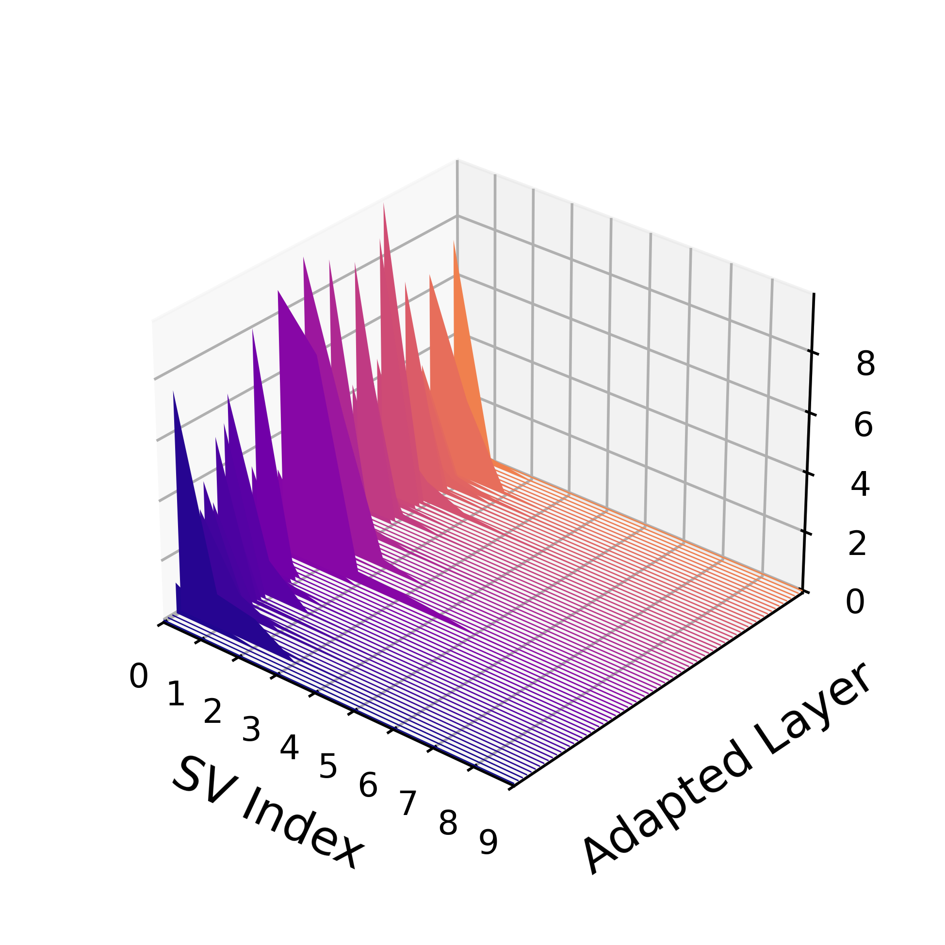
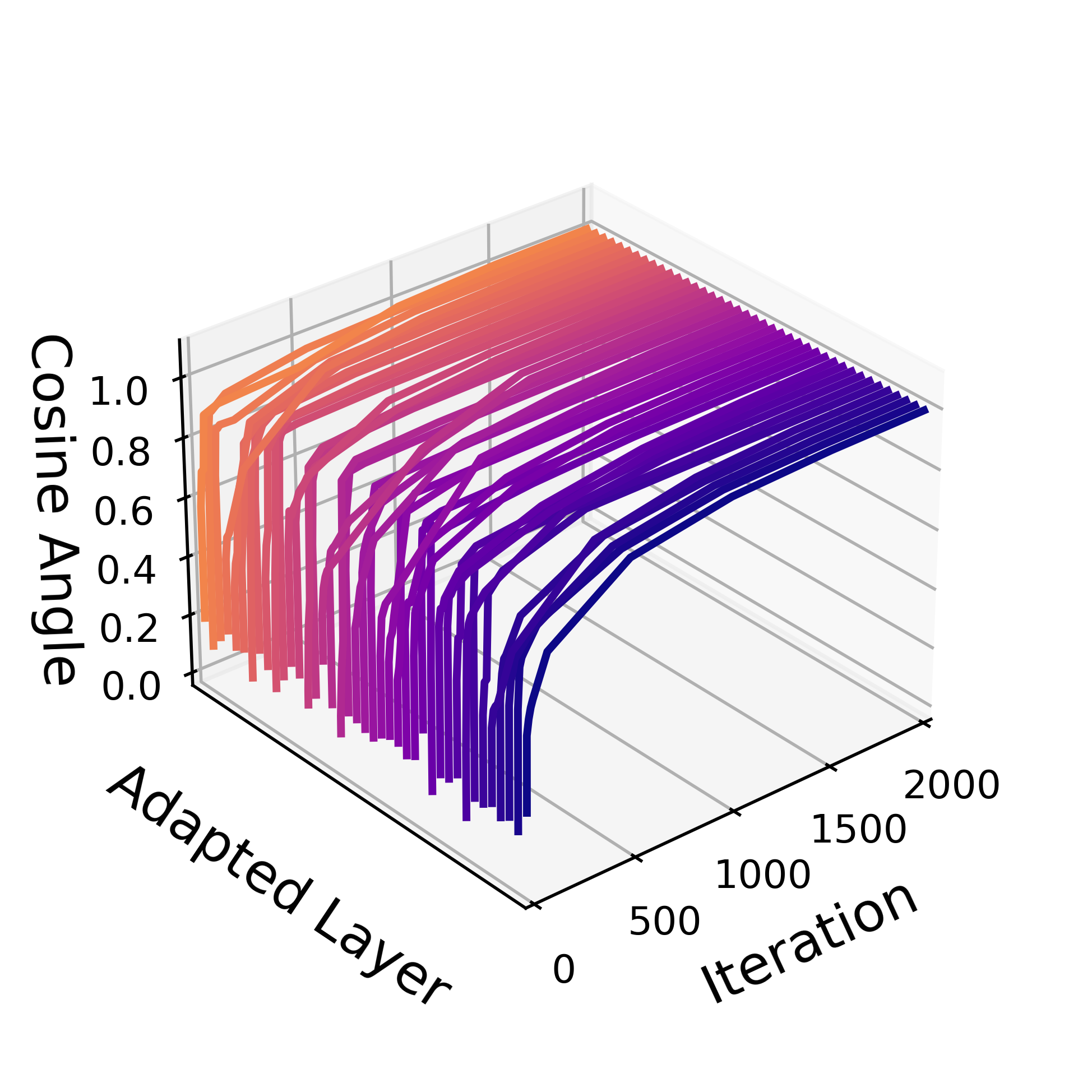
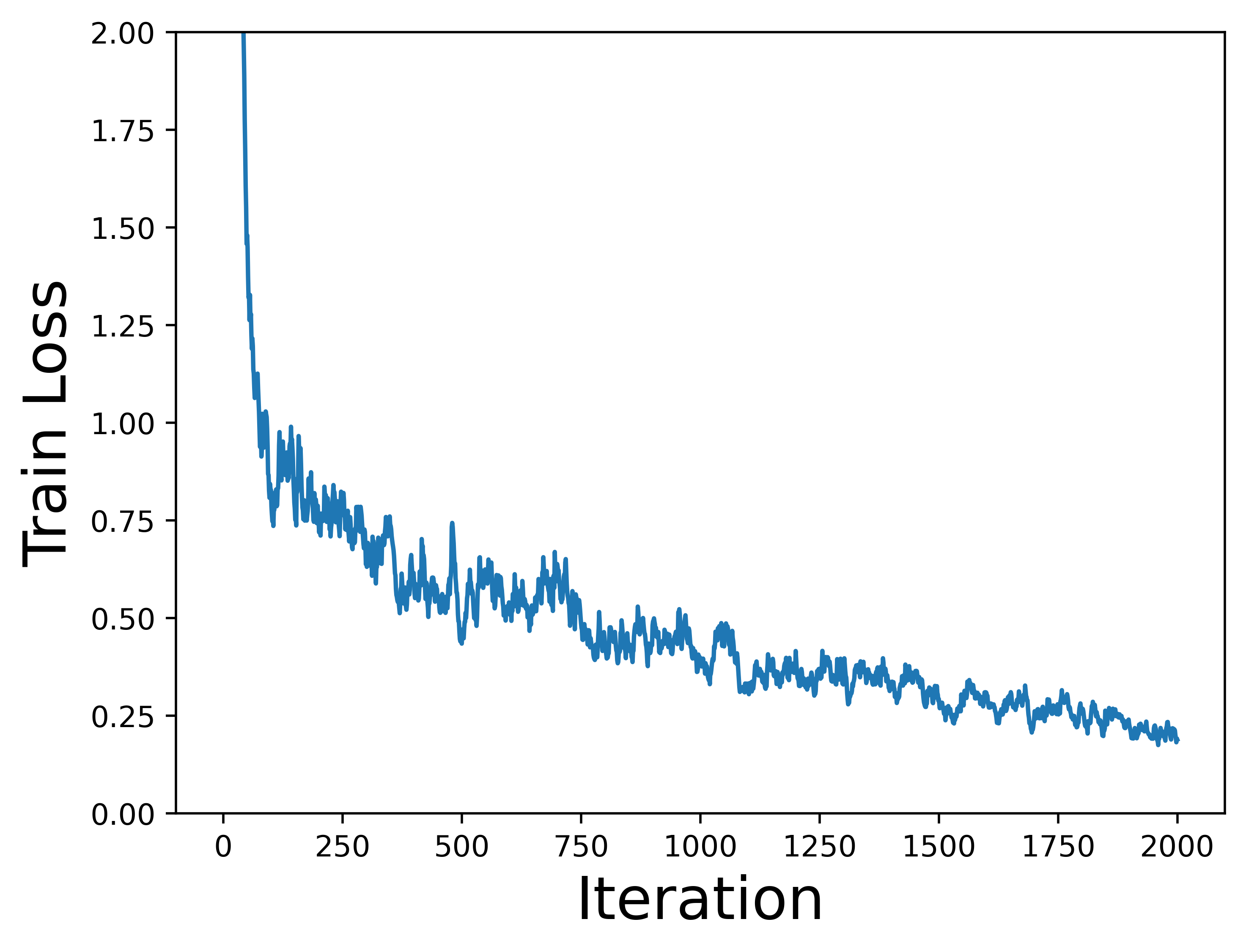
These unmodified panels were extracted from Yaras et al., Figure 2, under the PMLR CC BY 4.0 publication agreement. They are source-reported evidence, not a repository reproduction.

The three panels should not be collapsed:

small later singular values:
    numerical low-rank observation

high current-to-final subspace alignment:
    trajectory-direction observation under one metric

loss still decreasing:
    objective progress after alignment

The paper uses that observation to motivate Deep LoRA. The matrix-recovery theorem does not prove these BERT trajectories satisfy its exact block decomposition.

0x0AT Deep LoRA: From Full-Width Initialization To A Compact Trainable Graph

The paper’s method starts conceptually with a deeper update

$$\Delta W_k = W_k^{(L)}W_k^{(L-1)}\cdots W_k^{(1)}$$

whose uncompressed factors are full width. The pinned JAX/Flax reference implementation then constructs a compact module with

$$\Delta W = L_{out} \left( C_LC_{L-1}\cdots C_1 \right) R_{in}^{\top},$$

where

$$L_{out}\in\mathbb{R}^{d_{out}\times r}, \qquad R_{in}\in\mathbb{R}^{d_{in}\times r}, \qquad C_\ell\in\mathbb{R}^{r\times r}.$$

Its parameter ledger is

$$P_{Deep} = r(d_{out}+d_{in}) + Lr^2.$$

For the source’s usual depth $L=3$, this is vanilla LoRA’s two rectangular factors plus

$$3r^2$$

additional trainable parameters per adapted matrix.

For $d_{in}=d_{out}=8$ and $r=2$:

State	Parameters
Vanilla outer factors	$2(8)(2)=32$
Deep LoRA outer factors	$32$
Three $2\times2$ inner factors	$3(4)=12$
Deep LoRA total	$44$

That is parameter efficiency, not state equivalence. The deeper graph carries more activations, gradients, and optimizer tensors than vanilla LoRA.

0x0AU Pinned Code Trace: Compression Is An Initialization Pipeline

The reference code’s compressed path is not “instantiate a narrow deep factorization at random.” It performs a source-specific pipeline:

def initialize_compressed_deep_lora(base_model, first_batch, rank, depth):
    # 1. Materialize full-width, depth-L orthogonal factors.
    wide = build_full_width_deep_factors(depth=depth, scale=epsilon)

    # 2. Evaluate their end-to-end updates and one batch gradient.
    wide_update = multiply_factors(wide)
    wide_grad = grad(task_loss)(wide, first_batch)

    # 3. Move parameters, updates, and gradients to CPU/NumPy.
    left_basis, right_basis = gradient_informed_compression(
        wide, wide_grad, wide_update, rank
    )

    # 4. Keep rectangular outer factors and initialize each inner factor.
    compact.outer_left = left_basis            # [d_out, r]
    compact.outer_right = right_basis          # [d_in, r]
    compact.inner = [epsilon * I_r for _ in range(depth)]

    # 5. Use separate optimizer groups for outer and inner factors.
    return compact, multi_transform(inner_optimizer, outer_optimizer)

The implementation explicitly moves compression work to CPU to reduce GPU pressure. It also warns that creating the uncompressed factors can itself run out of memory before compression. Therefore the runtime contract includes a transient initialization peak:

$$M_{peak,init} \geq M_{base} + M_{wide\ factors} + M_{wide\ gradients} + M_{compression\ workspace}.$$

Only after compression does the steady trainable state become compact.

The code assigns a scaled learning rate to the outer factors and the main optimizer to the inner factors. Loop 7’s lesson applies directly: optimizer-group identity is part of the method, not incidental plumbing.

0x0AV Training And Runtime Integration Contracts

The source Deep LoRA experiment adapts all attention and feedforward weights in BERT-base, reports 72 adapted matrices, usually uses $r=8$, uses Adam, and compresses from a full-width depth-three orthogonal initialization with scale $10^{-3}$. Its limited-data experiments select learning rates under a declared protocol and train to convergence in training loss.

Those are source-reported choices, not defaults for another model. A faithful implementation record needs:

architecture state:
    exact adapted parameter paths and matrix orientations
    depth L, configured rank r, outer/inner shapes

compression state:
    first batch identity and preprocessing
    full-width initialization seed and epsilon
    gradient snapshot and compression code revision
    resulting outer bases and inner factors

optimizer state:
    inner and outer optimizer groups
    learning rates, decay, moments, step counters

checkpoint state:
    compact factors and group labels
    compression metadata and source revision
    base-model identity

serving state:
    materialized Delta W or live deep factor chain
    merge dtype and accumulation order
    latency measured separately from parameter count

M6.5 owns serving many adapters. This section only states why a deeper factor graph changes load, merge, and checkpoint semantics.

0x0AW Design Alternatives Answer Different Questions

Alternative	What changes	What it can answer	What it cannot inherit automatically
One matrix adapter	One additive gap	Exact rank and SVD tail	Deep function expressivity
Final-layer tuning	Dense freedom at the end	Whether one late map is enough	Distributed product budget
Uniform LoRA ranks	Same $R$ at every selected layer	Simple capacity ledger	Efficient allocation when gaps differ
Nonuniform ranks	Rank vector and partition	Coverage of heterogeneous gaps	Optimizer success
Constructive FNN/TFN adapters	Specific weights and biases	Existence under theorem assumptions	Reachability from LoRA initialization
NTK factorization	Linearized finite-data loss	Low-rank optimum and perturbed SOSP geometry	Unrestricted nonlinear training
Vanilla LoRA	Two-factor update	Low-state adaptation	Deep-factor implicit bias
Deep LoRA	Outer factors plus inner chain	Source method’s depth/compression tradeoff	Universal generalization gain

Final-layer tuning is especially instructive. Zeng and Lee show a random one-layer target cannot generically be matched by tuning only the final $L-1$ layers of their deeper frozen FNN, while distributed LoRA can meet their constructive conditions. The comparison is about where trainable changes enter the composition, not merely the count of scalar parameters.

0x0AX Paper-By-Contract Comparison

Paper	Mathematical object	Core rank statement	Optimization object	Strongest safe conclusion
Zeng—Lee expressive power	Product/FNN/TFN function equality	Gap rank distributed across layers; TFN bound through $G_i/2$	None	Constructed adapters exist under architecture and nonsingularity assumptions
Jang—Lee—Ryu NTK	Finite-data linearized loss	low-rank optimum with triangular count $\leq KN$; factor width with count $>KN$	Perturbed bilinear objective and SOSPs	A low-rank optimum exists and almost every declared perturbation removes nonglobal SOSPs
Yaras et al. matrix recovery	Deep square matrix product trajectory	active coordinate block width $2r$	GD from scaled-orthogonal initialization	The structured trajectory is compressible up to a finite-initialization bound
Yaras et al. Deep LoRA	Compressed deep adapter method	outer rank $r$ plus depth-$L$ inner chain	Source JAX/Flax training protocol	Source-reported limited-data behavior under one implementation and experiment

The papers are complementary because they study different missing links:

expressivity:
    can suitable adapters exist?

NTK optimization geometry:
    can a factorized linearized objective avoid bad SOSPs under a perturbation?

compressible dynamics:
    can one structured overparameterized GD trajectory be represented in fewer coordinates?

No row subsumes the others.

0x0AY Expressivity And Deep-Composition Failure Lab

Failure	Collapsed objects	Observable contradiction
$\operatorname{rank}(W_*-W_0)$ called the required LLM rank	one matrix vs deep function	another layer allocation reaches the same function with smaller per-layer rank
rank budgets called additive	upper bound vs equality	aligned terms fail to grow rank or cancel
FNN theorem applied with frozen biases	theorem construction vs implementation	intermediate ReLUs cannot be forced into the proof’s linear region
$D/2$ quoted without architecture	random no-residual theorem vs residual pretrained model	skip path and matrix shapes violate the formal setup
existence called trainability	representation vs optimizer trajectory	constructed solution exists but training does not reach it
$r=\lceil\sqrt N\rceil$ used as a recipe	asymptotic shorthand vs exact inequalities	$K$, triangular count, strictness, and perturbation disappear
P=0 called covered	perturbed theorem vs practical loss	theorem explicitly quantifies almost every nonzero PSD $P$
every stationary point called global	SOSP vs FOSP	negative-curvature first-order points are outside the conclusion
NTK theorem applied after large drift	linearized model vs nonlinear trajectory	Loop 8 linearization/Jacobian diagnostics fail
$2r$ invariant block called rank $r$	target rank vs active coordinate width	source decomposition has a $2r\times2r$ trainable block
compression called exact	small finite complement vs zero complement	residual equals $m\prod\epsilon_\ell^2>0$
BERT observation called theorem proof	source experiment vs matrix recovery	loss, optimizer, architecture, and initialization differ
compact parameters called low peak memory	steady state vs initialization lifecycle	full-width factors and gradients exist before compression
Deep LoRA merged like vanilla without metadata	two factors vs deep chain	checkpoint and optimizer-group state cannot be reconstructed

0x0AZ Loop 9 Handoff

Loop 9 closes four theorem boundaries:

1. a single matrix gap has an exact rank characterization;
2. depth can distribute a product gap under feasibility assumptions;
3. NTK low-rank existence and perturbed-landscape coverage use different inequalities and quantifiers;
4. invariant deep matrix dynamics and Deep LoRA language-model experiments are different evidence classes.

Loop 10 may now build the composite rank, reconstruction, kernel, and retention oracle. It must not convert theorem-sufficient rank into a practical selector, use the NTK result without Loop 8’s regime diagnostics, or treat source-reported Deep LoRA behavior as a local reproduction.

0x0B Rank, Reconstruction, Kernel, And Retention Oracle

The preceding loops deliberately refused to answer a deceptively simple question:

What LoRA rank should this product use?

That refusal was necessary. A singular-value tail answers a matrix approximation question. Principal angles answer a subspace question. Factor norms and gradients answer a trajectory question. A kernel comparison answers a conditional function-space question. An expressivity theorem answers an existence question under its assumptions. None of those objects, alone, selects a deployable rank.

Loop 10 joins them only after the training, validation, retention, stress, cost, checkpoint, and test contracts are immutable.

0x0BA Owner Contract: Select A Candidate, Not A Universal Rank

This section owns one bounded decision protocol:

input:
    a frozen candidate set
    matched training budgets
    validation-only checkpoint identities
    target, retention, and stress measurements
    reconstruction and trajectory diagnostics
    declared product constraints

output:
    one candidate selected for one release contract

not output:
    a universal LoRA rank
    a theorem-derived deployment recipe
    a reproduced paper benchmark
    a claim that low reconstruction error implies quality

The exact local oracle is synthetic. It validates the accounting and selection logic with rational values; it does not train a model. The Biderman et al. results remain source-reported empirical evidence.

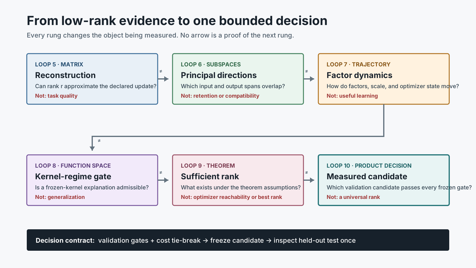
The ladder is intentionally not an implication chain. A candidate can have a small reconstruction residual and fail retention. It can remain near its initial kernel and fail to learn. It can satisfy a theorem’s sufficient rank and still be unnecessarily expensive or unreachable by the chosen optimizer.

0x0BB Why Rank Adequacy Is A Product Decision

Let candidate $i$ have validation target score $S_i$, retained base score $R_i$, stress score $U_i$, and cost $C_i$. Assume all three quality metrics are higher-is-better. Relative to the frozen base candidate $0$, define target gain

$$G_i = S_i-S_0$$

and forgetting

$$F_i = R_0-R_i.$$

This sign convention matters. Positive $F_i$ means the adapted candidate retained less of the measured base behavior. If a retention metric is lower-is-better, it must first be oriented or normalized; silently mixing directions makes the tradeoff plot meaningless.

A low-rank run can therefore occupy at least four distinct states:

Target gain	Forgetting	Interpretation
high	low	strong candidate under the measured axes
high	high	useful adaptation with a retention cost
low	low	constrained movement; possibly underfitting
low	high	dominated failure

“Forgets less” is not automatically a success. If $G_i$ does not meet the product floor, low forgetting describes failure to adapt, not an efficient release.

0x0BC Reconstruct The Source Experiment Before Quoting It

Biderman et al. compare LoRA with full fine-tuning for Llama-2-7B across two domains and two training regimes:

Axis	Source contract
domains	programming and mathematics
regimes	continued pretraining and instruction fine-tuning
continued-pretraining data	StarCoder-Python and OpenWebMath, up to 20B training tokens
instruction data	Magicoder-Evol-Instruct-110K and MetaMathQA, about 100K prompt-response pairs
LoRA ranks	16, 64, and 256
scale	$\alpha=2r$, so $\alpha/r=2$ across the rank sweep
dropout	’lora_dropout = 0.05’
adapted module families	query, key, value, output, gate, up, and down projections
code target metric	HumanEval pass@1 under the paper’s generation protocol
mathematics target metric	GSM8K pass@1 under the paper’s prompting protocol
retention metrics	HellaSwag, WinoGrande, and ARC-Challenge accuracies

This matrix blocks several invalid summaries. The paper did not test every model family, every rank, every adaptation surface, every domain distance, or every serving constraint. Its CPT and IFT conclusions are not interchangeable.

0x0BD The Source Tradeoff Is Empirical, Not An Algebraic Consequence

The paper reports that standard low-rank LoRA often learned less of the target domain than full fine-tuning in the studied settings, while retaining more out-of-domain behavior. Higher rank generally increased target learning and also changed forgetting. The exact tradeoff depended on domain and training regime.

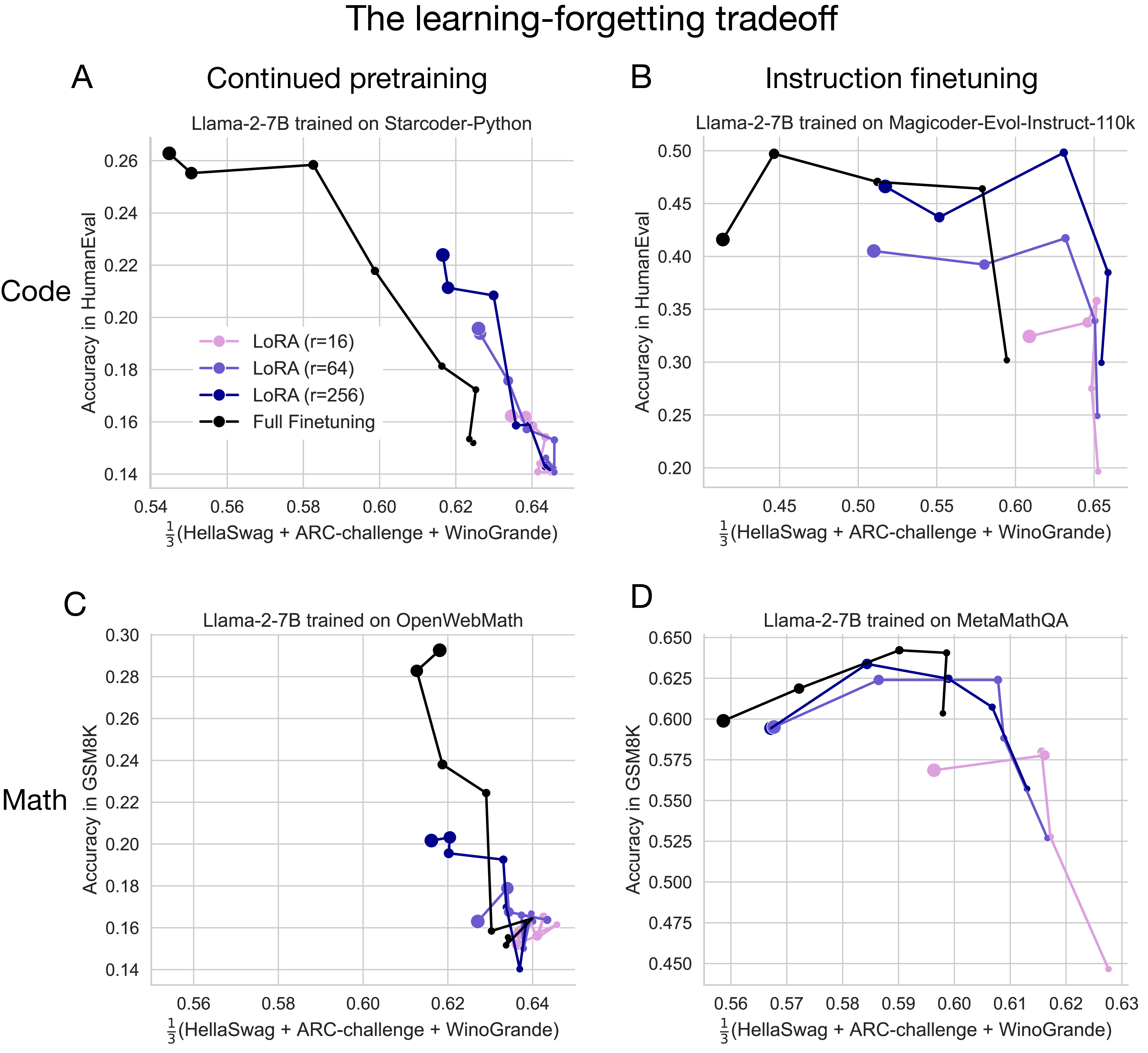
Source-reported Biderman et al. Figure 3, extracted from the version-2 paper image stream under CC BY 4.0. The repository did not digitize the plotted values or reproduce the training runs.

The four panels are important because there is no single “LoRA frontier.” Code CPT, code IFT, mathematics CPT, and mathematics IFT place the same method names on different surfaces. Some high-rank instruction-tuning runs approach or match the target score of full fine-tuning while retaining more base behavior; some continued-pretraining settings preserve a substantial target gap.

0x0BE Derive The Full-Update Rank Measurement

For one frozen weight $W_0$ and its full-fine-tuned checkpoint $W_{ft}$, define

$$\Delta W_{ft}=W_{ft}-W_0.$$

If

$$\Delta W_{ft}=U\operatorname{diag}(\sigma_1,\ldots,\sigma_q)V^{\top}, \qquad \sigma_1\ge\cdots\ge\sigma_q\ge 0,$$

then the smallest rank explaining fraction $\rho$ of squared Frobenius energy is

$$r_{\rho} = \min\left\{ r: \frac{\sum_{j=1}^{r}\sigma_j^2} {\sum_{j=1}^{q}\sigma_j^2} \ge \rho \right\}.$$

The source uses $\rho=0.9$ for its layerwise full-update analysis. This is an energy-prefix rank, not algebraic rank, numerical rank, stable rank, configured LoRA rank, or the smallest rank that reaches a task score. Loop 5 derived those policies separately because their values need not agree.

0x0BF Full-Update Rank Varies Across Layer, Module, And Time

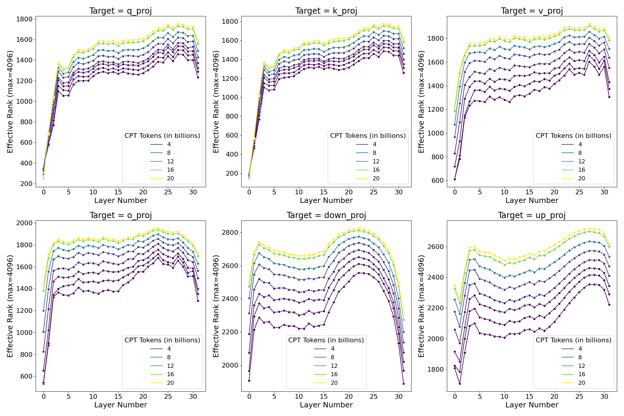
Source-reported Biderman et al. Figure 6, extracted from the version-2 paper image stream under CC BY 4.0. The y-axis is the rank needed to explain at least 90% of full-update variance; it is not a recommended LoRA rank.

The source reports three patterns in its code continued-pretraining run:

1. measured full-update rank grows over training;
2. MLP updates generally have higher energy ranks than attention updates; and
3. middle layers often have higher ranks than boundary layers.

The earliest analyzed checkpoint already has 90%-energy ranks far above common LoRA configurations. That observation can explain a capacity gap, but it does not prove that no lower-rank task-sufficient solution exists. The full-update optimizer found one high-rank path. A different parameterization can reach a different update with similar outputs.

0x0BG The Immutable Run Manifest

Before training, freeze a row for every candidate:

candidate_id
base_model_id / tokenizer_id
method / configured rank / target-module surface
alpha / dropout / initialization
optimizer / schedule / precision / clipping
train dataset payload hash / sample order / token budget
seed / world size / gradient accumulation
checkpoint cadence / selection rule
target-validation split and metric revision
retention-validation split and metric revision
stress-validation split and metric revision
held-out test split identities
diagnostic probe identities
trainable-state and peak-memory accounting

Rank without surface is incomplete. Rank 16 on query and value projections is not the same capacity, cost, or function class as rank 16 on all attention and MLP projections. M6.4 owns the variant mechanisms; this loop records their changed objects as candidate metadata.

0x0BH Run And Artifact Identity Must Survive Resume

One logical run produces many artifacts:

run identity
    -> training configuration
    -> optimizer and scheduler state
    -> candidate checkpoints
    -> validation score records
    -> full-update deltas and spectra
    -> subspace / factor / kernel diagnostics
    -> selected release checkpoint
    -> held-out test report

The checkpoint selected on validation must retain the exact optimizer, dataset, seed, and metric lineage that produced it. A filename such as ‘lora_rank_16_final.pt’ is not enough. If a resumed run changes sample order, precision, target surface, or checkpoint-selection code, it is a new candidate identity.

0x0BI Checkpoint Selection Is Nested Inside Rank Selection

Let $\mathcal{C}_i$ be the checkpoints for candidate $i$. A predeclared validation rule chooses

$$c_i^* = \operatorname{SelectCheckpoint} \left( \{c\in\mathcal{C}_i\}; S_{i,c}^{val},R_{i,c}^{val},U_{i,c}^{val} \right).$$

Only then may ranks be compared:

$$i^* = \operatorname{SelectCandidate} \left( \{c_i^*\}_i; \text{frozen validation policy} \right).$$

Using test performance to choose either $c_i^*$ or $i^*$ leaks the final evaluation into model selection. “We only looked once” is still leakage if the result changes the chosen rank.

0x0BJ One Candidate Record Joins, But Does Not Collapse, The Evidence

The candidate record is a typed product:

Field family	Consumed result	Forbidden inference
reconstruction	Loop 5 rank, singular tail, sampled-output residual	low task loss
subspace	Loop 6 row/column angles and directed coverage	retention
trajectory	Loop 7 factor norms, gradients, scale, optimizer, dtype state	useful feature learning
function space	Loop 8 Jacobian, kernel, and linearization diagnostics	generalization
theorem scope	Loop 9 assumptions and sufficient-rank statements	practical optimum
operational scores	target, retention, stress, cost, uncertainty	universal rank

Joining means every field shares one candidate identity. It does not mean the fields are interchangeable.

0x0BK Seed Aggregation And Uncertainty Are Part Of The Metric

For $n$ declared seeds and score $S_{i,s}$,

$$\bar S_i=\frac{1}{n}\sum_{s=1}^{n}S_{i,s},$$

with sample variance

$$s_{S_i}^2 = \frac{1}{n-1} \sum_{s=1}^{n} \left(S_{i,s}-\bar S_i\right)^2.$$

When seeds or evaluation items are paired, compare paired differences

$$d_s=S_{i,s}-S_{j,s}, \qquad \bar d=\frac{1}{n}\sum_s d_s$$

rather than pretending two independent error bars describe the difference. Publish a confidence or bootstrap interval whose resampling unit matches the actual dependence structure. Three seeds with a narrow observed range are not proof of a narrow population interval.

The exact oracle reports mean, minimum, maximum, and range only. Those are deterministic fixture summaries, not confidence intervals.

0x0BL Forgetting Must Name A Baseline And A Metric Direction

For higher-is-better retention score $R$, the oracle uses

$$F_i=R_0-R_i.$$

If the base scores 90 and a candidate scores 85, forgetting is 5 points. For a lower-is-better loss $L$, the oriented degradation would instead be

$$F_i^{loss}=L_i-L_0.$$

Do not average raw heterogeneous metrics. The Biderman paper’s plotted retention axis averages three accuracies with the same direction. A product suite mixing accuracy, toxicity, latency, and calibration error needs separate units or an explicitly frozen normalization.

0x0BM Reconstruction Is A Gate, Not The Objective

Loop 5’s exact matrix has Frobenius tail squares

$$30,\ 14,\ 5,\ 1,\ 0$$

at ranks $0,1,2,3,4$. Under its identity-input probe, mean output residuals are

$$5,\ \frac{7}{3},\ \frac{5}{6},\ \frac{1}{6},\ 0.$$

Loop 10 consumes those values by digest and object identity. It does not recompute them under a new convention. In the fixture, a reconstruction gate requires

$$\left\|\Delta W-\Delta W_r\right\|_F^2\le 5.$$

Rank 2 passes exactly. That still does not select rank 2: target, retention, stress, budget, and diagnostic gates must also pass.

0x0BN Subspace, Dynamics, And Kernel Checks Are Admissibility Checks

A candidate may be compared in subspace only after rank-revealing orthonormalization and gauge removal. A candidate may be interpreted through a fixed kernel only if the frozen probe, output coordinates, optimizer metric, Jacobian drift, kernel drift, alignment, and output linearization residual are all recorded.

The oracle therefore evaluates

kernel_gate = (
    not candidate.kernel_interpretation_requested
    or candidate.kernel_bundle_complete
)

It contains no universal “small drift” threshold. The threshold, horizon, probe, and estimator belong to the study manifest. A missing kernel bundle invalidates the kernel explanation; it does not automatically invalidate the candidate’s measured target score.

0x0BO Theorem Rank Cannot Enter The Tie-Breaker

Loop 9 produced sufficient-rank statements for specific matrix, FNN, Transformer, and linearized NTK contracts. Those ranks cannot be inserted into the candidate selector because they answer different objectives and may not prove reachability by the actual optimizer.

The fixture requires

theorem_rank_used_as_selector = false

for every candidate. Theorems can motivate sweep boundaries or explain a result after assumptions are checked. They cannot replace measurement.

0x0BP Pareto Dominance Preserves The Tradeoff Geometry

With target, retention, and stress higher-is-better and cost lower-is-better, candidate $i$ weakly dominates $j$ when

$$S_i\ge S_j,\qquad R_i\ge R_j,\qquad U_i\ge U_j,\qquad C_i\le C_j,$$

and at least one inequality is strict. The Pareto set is

$$\mathcal{P} = \left\{ i: \nexists j\text{ that dominates }i \right\}.$$

This operation needs no arbitrary conversion between “one retention point” and “one megabyte.” It removes strictly inferior candidates while preserving the remaining product tradeoffs.

0x0BQ A Constrained Selector Makes Product Requirements Explicit

Let the validation floors be $\tau_S,\tau_R,\tau_U$, let the maximum reconstruction residual be $\tau_E$, and let $D_i$ mean all required diagnostic and budget checks pass. The feasible set is

$$\mathcal{F} = \left\{ i: S_i\ge\tau_S,\ R_i\ge\tau_R,\ U_i\ge\tau_U,\ E_i\le\tau_E,\ D_i=1 \right\}.$$

The exact fixture then applies a lexicographic rule:

$$i^* = \arg\min_{i\in\mathcal{F}} \left(C_i,r_i,\operatorname{id}_i\right).$$

This means: meet quality first, then choose the least costly eligible candidate, then the smaller configured rank, then a deterministic identifier. It does not reward exceeding one quality floor enough to compensate for violating another.

0x0BR Exact Validation Oracle

The local fixture freezes

$$\tau_S=72,\qquad \tau_R=84,\qquad \tau_U=88,\qquad \tau_E=5.$$

Its validation means are:

Candidate	Rank	Target	Retention	Stress	Forgetting	Cost	Tail $E_i$	Feasible
base	n/a	50	90	78	0	0	30	no
LoRA r1	1	62	88	82	2	8	14	no
LoRA r2	2	74	85	89	5	16	5	yes
LoRA r3	3	73	82	88	8	24	1	no
LoRA r4	4	82	74	90	16	32	0	no
full FT	n/a	88	65	93	25	120	0	no

The numbers are pedagogical inputs. Their value is that the decision can be audited exactly:

1. rank 1 fails target, stress, and reconstruction;
2. rank 2 passes every gate;
3. rank 3 has a better matrix residual but fails retention and lacks the requested kernel bundle;
4. rank 4 and full fine-tuning improve target score but violate retention; and
5. therefore only rank 2 is feasible under this product contract.

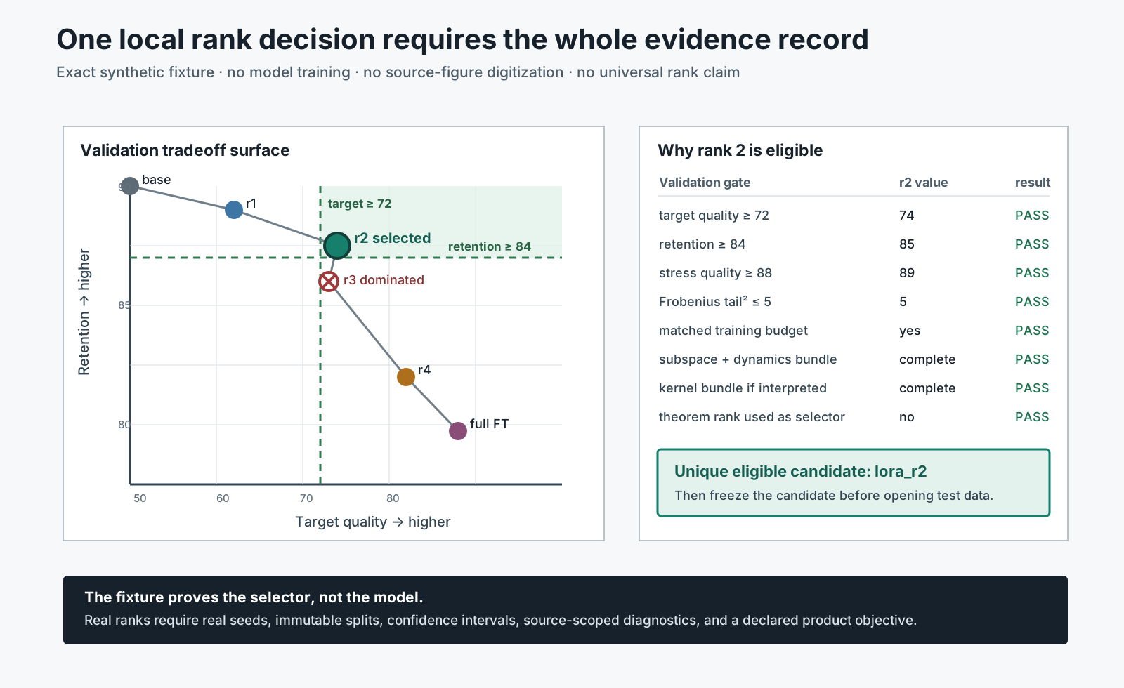
0x0BS The Frontier And The Feasible Set Are Different

The exact four-objective frontier is

base
lora_r1
lora_r2
lora_r4
full_ft

‘lora_r3’ is dominated by ‘lora_r2’: it has lower target, retention, and stress means while costing more. The other candidates remain Pareto-relevant because each preserves a different extreme. Yet only ‘lora_r2’ belongs to the feasible set.

This distinction prevents two common errors:

Pareto-optimal
    does not mean deployable

constraint-feasible
    does not mean globally best under another product contract

Changing the retention floor can change the selection without changing any model. That is policy sensitivity, not model instability.

0x0BT Held-Out Test Is A Report, Not Another Selection Round

After selecting ‘lora_r2’, the fixture opens the held-out test report:

Candidate	Test target	Test retention	Test stress
base	49	90	78
selected LoRA r2	73	85	88
full-FT reference	87	64	92

The selector does not run again. If the selected candidate fails a predeclared release gate on test, the outcome is no release or a new versioned study, not “pick the runner-up using test.”

0x0BU Executable Selection Trace

manifest = load_immutable_manifest()
assert disjoint(manifest.validation_splits, manifest.test_splits)
assert not test_store.was_opened()

records = []
for candidate in manifest.candidates:
    checkpoints = train_or_load(candidate)
    chosen = select_checkpoint(checkpoints, candidate.validation_rule)

    record = {
        "candidate_id": candidate.id,
        "checkpoint_id": chosen.id,
        "target": evaluate(chosen, manifest.target_validation),
        "retention": evaluate(chosen, manifest.retention_validation),
        "stress": evaluate(chosen, manifest.stress_validation),
        "cost": account_trainable_and_runtime_state(chosen),
        "reconstruction": run_reconstruction_protocol(chosen),
        "subspace": run_subspace_protocol(chosen),
        "dynamics": load_training_trajectory(chosen),
        "kernel": run_kernel_bundle_if_requested(chosen),
    }
    records.append(record)

frontier = pareto_frontier(records, manifest.objective_directions)
feasible = [row for row in records if passes_every_gate(row, manifest)]
if not feasible:
    # No candidate passes every gate: fail closed with no release.
    # Nothing is frozen and the held-out test store stays closed.
    record_no_release(manifest.digest)
    raise SystemExit("no release: the feasible set is empty")
selected = min(feasible, key=lambda row: (
    row["cost"],
    configured_rank_or_infinity(row),
    row["candidate_id"],
))

freeze(selected["candidate_id"], selected["checkpoint_id"], manifest.digest)
assert not test_store.was_opened()
test_report = evaluate_frozen_release(selected, test_store.open_once())

Production code should fail closed on missing metrics, mixed revisions, NaNs, unknown directions, duplicate candidate IDs, or a test-store access event.

0x0BV Artifact And Runtime Integration

The release candidate needs more than adapter tensors:

selection manifest digest
base model and tokenizer identity
adapter checkpoint and target-module map
optimizer/checkpoint lineage
validation score records with raw per-seed outputs
retention and stress suite revisions
reconstruction/subspace/kernel diagnostic artifacts
trainable-state, peak-memory, and wall-time ledgers
selected candidate and tie-break trace
held-out test access record
rollback candidate identity

M6.5 owns multi-adapter serving and M6.9 owns routed composition. Loop 10 only requires that any runtime state used as a cost or release gate be measured under a pinned deployment contract rather than inferred from rank alone.

0x0BW Alternative Decision Designs

Design	Useful when	Main risk
hard constraints then minimum cost	product floors are real requirements	feasibility can be sensitive near thresholds
Pareto frontier plus human choice	tradeoffs cannot be scalarized honestly	decision may be hard to automate
weighted utility	units and business weights are stable	hidden weights can manufacture a winner
knee-point selection	smooth frontier has a meaningful curvature	scaling and normalization change the knee
confidence-bound selection	uncertainty is material	interval and dependence assumptions must be valid
sequential racing	large candidate grid is expensive	early noisy metrics can eliminate the best run

This article uses hard constraints because every pass/fail condition is visible. It refuses an undeclared scalar score such as

$$S_i+R_i+U_i-C_i$$

because the units and weights have no natural equality.

0x0BX Paper-By-Contract Comparison

Evidence	Object	What it supports	What remains unproved
LoRA	learned low-rank perturbations on selected matrices	low-rank adaptation can be competitive in tested tasks	universal adequate rank
Biderman et al.	Llama-2-7B LoRA/full-FT learning and forgetting experiments	source-scoped target/retention tradeoffs and full-update spectra	that high full-update rank is necessary for task success
Loop 5 / Eckart—Young	one declared matrix and norm	best post-hoc rank-$r$ approximation	LoRA optimizer convergence or task quality
Loop 6	update row/column spaces	gauge-invariant subspace comparison	retention or compatibility
Loop 7	factor-coordinate dynamics	exact local trajectory and conditioning facts	general AdamW behavior without its state
Loop 8 / kernel sources	finite-data Jacobian and kernel objects	conditional fixed-kernel interpretation	useful feature learning or generalization
Loop 9 theorem sources	source-specific existence and landscape statements	sufficient ranks under quantified assumptions	practical candidate selection
Loop 10 exact fixture	declared validation measurements and policy	deterministic selector and failure rejection	any paper benchmark or universal rank

0x0BY Rank And Retention Failure Lab

Failure	Hidden collapse	Consequence
choose rank from $r_{0.9}$ alone	full-update reconstruction vs task solution	excessive or insufficient adapter
praise low forgetting without target floor	retention vs underfitting	product learns too little
select best test score	evaluation vs model selection	optimistic final estimate
compare ranks with different surfaces	rank vs trainable function class	capacity and cost are confounded
pick best checkpoint independently on test	checkpoint vs rank nesting	double selection leakage
average metrics with mixed directions	score orientation omitted	reversed Pareto relation
use one aggregate without units	tradeoff vs arbitrary scalarization	invisible product weights
call overlap retention	update geometry vs behavior	false compatibility claim
call kernel alignment quality	mechanism vs utility	stable but poor model accepted
use theorem rank as tie-breaker	sufficient existence vs measurement	assumptions replace evidence
omit failed or missing diagnostics	unknown vs pass	incomplete candidate enters release
rerun selection after test failure	test report vs new study	held-out set becomes validation
ignore seed or item dependence	variation vs independent evidence	confidence is overstated
promote one fixture rank	local oracle vs empirical law	rank 2 becomes a false recipe

0x0BZ Loop 10 Handoff

The fixture proves the selector, not the model.

Loop 10 closes the rank-selection algebra:

1. five predecessor reports are consumed by immutable digest rather than reinterpreted;
2. target learning and retention use explicit baselines and directions;
3. checkpoint selection is nested inside candidate selection;
4. Pareto and constraint feasibility remain different objects;
5. test data cannot alter the selected rank;
6. the exact fixture rejects every one-field contract mutation; and
7. source figures remain empirical evidence rather than local reproduction.

Loop 11 may now expand the failure lab, complete source and visual provenance, add responsive variants, and turn the experimental protocol into release-facing checklists. It must not reopen test data as a selector or convert the exact fixture’s rank 2 into advice.

0x0C Failure Closure, Complete Evidence, And Experimental Design

Loop 10 proved that a frozen policy can join heterogeneous diagnostics without turning any one diagnostic into the objective. It did not establish that a real rank comparison has been designed correctly. A candidate table can be algebraically valid while its runs differ in data order, initialization, checkpoint opportunity, target modules, failed-run handling, or test exposure. Those differences can dominate the rank coordinate that the table claims to study.

Loop 11 therefore closes two different surfaces:

1. every mechanism failure from Loops 2—10 receives a typed detector, consequence, and recovery owner; and
2. a future empirical rank study receives an immutable design whose units, treatments, blocks, nuisance variables, estimands, stopping rules, and release decisions are fixed before outcomes are inspected.

The local fixture remains synthetic. It validates the design transaction; it does not execute the proposed training runs or supply evidence that one rank is best.

0x0CA Owner Contract: Close Evidence Without Inventing A Rank Benchmark

M6.7 owns the relation between a low-rank claim and the evidence needed to test it. In this loop that includes:

typed failure identity and bounded recovery
experiment unit, treatment, block, nuisance coordinate, and estimand
paired candidate comparison and incomplete-pair policy
seed, data-order, split, checkpoint, and evaluator provenance
validation-only selection and held-out-test isolation
static source, local-link, figure, visual, and negative-test closure

It still does not own adapter runtime residency, learned adapter routing, generic deployment packaging, or general scaling-law extrapolation. Those remain M6.5, M6.9, M8, and M4.7—M4.9 respectively. A failure record can hand an issue to those owners; it cannot absorb their mechanisms into this article.

0x0CB A Failure Record Needs Seven Coordinates

A prose warning such as “rank may be too small” cannot be tested or recovered. The machine-readable failure manifest gives each failure seven coordinates:

failure id and alarm family:
    stable identity plus the class of state or claim that became unsafe

origin loop and invariant:
    the first mechanism contract that must remain true

perturbation:
    one concrete drift that can violate the invariant

detector:
    an equality, digest, rank check, directional derivative, split audit,
    completeness test, or bounded discrepancy

consequence:
    the first derived result that can no longer be trusted

recovery owner:
    the only article, experiment stage, or release gate allowed to repair it

evidence limit:
    what a successful detector still does not prove

The final coordinate prevents a common escalation error. Exact finite-matrix parity proves an algebraic identity, not language-model quality. A complete source manifest proves provenance, not live network availability. A green static SVG audit proves structure, not mobile legibility.

0x0CC Six Alarm Families Must Remain Distinct

The closure manifest has four failures for each mechanism loop from Loop 2 through Loop 10. Its thirty-six records belong to six alarm families:

Alarm family	Representative invariant	Detector	Typical recovery
identity and protocol	base, tensor, split, rank policy, and protocol IDs denote the same study objects	manifest digest, axis, split, and object-join audit	reject the run or rebuild the manifest before execution
geometry and reconstruction	rank, tangent, SVD, covariance support, and subspace metrics use their declared objects and thresholds	exact rank/projector/residual oracle	recompute the diagnostic; never relabel it
optimization and numerics	factor gauge, initialization, scaling, optimizer metric, and dtype path match the derived dynamics	gradient, product-velocity, range, and resume checks	restore factors/optimizer state or narrow the claim
function space and theorem	Jacobian, kernel, linearization horizon, theorem assumptions, and practical decision remain separate	current-versus-frozen trajectory and assumption ledger	invalidate the explanation, not the observed score
experimental design and statistics	candidate cells are paired, complete, validation-only, and direction-aware	design-cell, checkpoint, estimand, and test-access audit	no selection; version a new study if policy changes
evidence, publication, and release	sources, figures, URLs, artifacts, and evidence classes are complete and correctly scoped	provenance, digest, route, and claim-firewall audit	repair metadata or block publication/release

No alarm substitutes for another. A passed SVD residual cannot repair a split leak. A paired score interval cannot establish a tangent-space theorem. A source-reported paper figure cannot validate the local selection oracle.

0x0CD Same Shape, Same Mean, And Same Seed Count Are Not Same Evidence

Several dangerous substitutions preserve the headline dimensions:

Superficially equal object	Hidden mismatch	Required check
two $d_{out}\times d_{in}$ deltas	different base checkpoint or tensor orientation	base/tensor identity plus executable output trace
two rank-$r$ products	different row/column spaces or numerical rank	spectrum and separate row/column projectors
two candidate means	different seed tuples, missing runs, or checkpoint opportunity	paired-cell completeness and attempt lineage
two four-seed studies	one varies initialization, the other data order	explicit nuisance-coordinate manifest
two retention scores	different base metric or higher/lower-is-better convention	baseline and metric-direction record
two validation tables	one chose hyperparameters after viewing test	access log and frozen-candidate transaction
two successful reruns	one silently dropped an earlier failed attempt	immutable run ID with every attempt and termination reason

Even output equality at one probe is insufficient. Gauge-equivalent factors can compute the same product and take different optimizer steps. Two kernels can have high normalized alignment and different scale. A base model and an untrained zero-product LoRA branch can emit the same tensor while owning different gradients and artifact state.

0x0CE Define Unit, Treatment, Block, Nuisance, And Estimand First

The word “run” is too vague for an experimental record. One training unit is:

$$u_{c,b,s,j} = (c, b, s_{init}, s_{order}, s_{dropout}, j),$$

where $c$ is the candidate pipeline, $b$ is a frozen experimental block, $s=(s_{init},s_{order},s_{dropout})$ is a nuisance tuple, and $j$ is a predeclared checkpoint step. The block includes domain, training regime, data budget, target-module surface, tokenizer/data revisions, base checkpoint, and evaluator revision.

The candidate is not “rank” unless every other treatment coordinate is fixed. If rank 16 also uses another target-module set, scale rule, optimizer schedule, or quantized base, the treatment is the whole pipeline:

$$c=(r,\mathcal{T},s(r),\mathcal{O},\mathcal{I},\mathcal{Q}),$$

with target set $\mathcal{T}$, branch scale $s(r)$, optimizer $\mathcal{O}$, initialization $\mathcal{I}$, and base representation $\mathcal{Q}$. Calling the resulting contrast a pure rank effect would be wrong.

For one outcome $Y$, a bookkeeping model can expose the design coordinates:

$$Y_{c,b,s} = \mu+\tau_c+\beta_b+\gamma_{s_{init}}+\delta_{s_{order}} +\zeta_{s_{dropout}}+\iota_{c,b,s}.$$

This equation is an index decomposition, not an assertion that the effects are additive or Gaussian. Interactions remain in $\iota$. Its purpose is to stop a nuisance change from being silently attributed to $\tau_c$.

0x0CF Pair Candidates Across Nuisance Coordinates

When two candidate pipelines can share a nuisance tuple, the primary contrast should preserve that pairing:

$$D_{c,c',b,s}=Y_{c,b,s}-Y_{c',b,s}, \qquad \widehat{\Delta}_{c,c',b} = \frac{1}{|S_b|}\sum_{s\in S_b}D_{c,c',b,s}.$$

The paired contrast removes variation common to the same block and nuisance tuple. It does not remove interactions between candidate and seed. If one side is missing, that pair is incomplete; substituting another seed breaks the pairing. A missing-cell policy must be frozen before outcomes are visible.

The base checkpoint is a deterministic baseline record rather than a fake training replicate. Full fine-tuning and LoRA can share data order, dropout, and optimizer RNG identities even though their trainable state differs. Any coordinate that cannot be meaningfully paired is named and analyzed as an unpaired source of variation.

Fine-tuning variance is not hypothetical. Dodge et al. varied weight initialization and data order across 2,100 BERT fine-tuning trials and reported that both contributed materially to outcome variation. Reimers and Gurevych showed in sequence tagging that one selected random seed could change the apparent method ranking and argued for score distributions rather than one score. These are source-reported results on their tasks, not variance estimates for this proposed study.

0x0CG A Seed Range Is Not A Confidence Interval

There are at least three sampling levels:

training-run level:
    initialization, data order, dropout, kernels, and optimizer trajectory

evaluation-item level:
    prompts, examples, tasks, users, domains, or generated samples

study-design level:
    split construction, data budget, hyperparameter search, checkpoint grid,
    candidate family, and evaluator revision

For paired candidate differences $D_s$, the run-level sample variance is:

$$\widehat{V}_{run} = \frac{1}{S-1}\sum_{s=1}^{S}(D_s-\bar D)^2.$$

It estimates dispersion over the declared nuisance-tuple population only when those tuples were sampled under the stated design. The minimum and maximum of four seeds are descriptive endpoints, not a confidence interval. Treating thousands of test items from one trained checkpoint as thousands of independent training runs is pseudoreplication.

If a metric has valid item-level contributions, an item bootstrap should keep candidate predictions paired on the same resampled items. To combine item and run variation, a hierarchical procedure first resamples nuisance tuples and then paired items within the chosen tuple. Metrics such as pass@$k$, correlated task suites, or judge-based scores need estimator-specific resampling; the article does not prescribe one universal bootstrap.

Bouthillier et al. model benchmarking as a pipeline with variation from data sampling, initialization, and hyperparameter choice. Their result supports exposing multiple variation sources; it does not prove that the additive bookkeeping equation above is a correct stochastic model for LoRA ranks.

0x0CH Selection Creates Multiplicity And Optimism

Rank, checkpoint, target modules, scale, and optimizer settings form a search family. Reporting the best validation value as if it were one prespecified measurement ignores selection. The immutable protocol therefore records:

1. the candidate and checkpoint family before training;
2. the metric directions and product gates before selection;
3. the tuning budget allocated to every candidate;
4. the selection rule, tie-breaker, and missing-run policy;
5. the single frozen candidate identity before test access.

Comparing many ranks may require simultaneous intervals, a family-wise error procedure, false-discovery control, or an explicitly descriptive decision analysis. The correct method depends on the hypothesis, paired structure, metric distribution, and number of comparisons. Dror et al. make the same general point for NLP significance testing: test choice depends on the experimental setup and evaluation measure. A star beside one metric is not a universal evidence contract.

Test failure does not authorize selecting the validation runner-up. The valid outcomes remain release or no release. Changing the candidate family, gates, test interpretation, or retry policy creates a new versioned study with new held-out data.

0x0CI Early Stopping, Missing Runs, And Retries Need Attempt Lineage

Early stopping can save compute, but it is part of the candidate pipeline. The monitor, direction, patience, minimum delta, checkpoint cadence, warmup, and maximum step must be predeclared and validation-only. A rule cannot inspect a test metric, and failed candidates cannot be removed merely because they lower the mean.

Every training unit owns one immutable run_id and one or more attempt IDs:

run_id:
    candidate + block + nuisance tuple

attempt_id:
    run_id + retry ordinal + environment digest

termination class:
    completed, validation-stopped, numerical failure,
    infrastructure failure, admission failure, or operator cancellation

retry rule:
    infrastructure-only under the same semantic run identity;
    preserve the failed attempt and never choose the better retry by score

A numerical divergence is an outcome of the pipeline, not an infrastructure retry. An interrupted run may resume only from an exact state bundle whose optimizer, scheduler, scaler, RNG, sampler, counters, and data position restore before the next stochastic event.

0x0CJ Immutable Experimental-Design Manifest

Before the first outcome is observed, freeze:

question, primary estimands, secondary diagnostics, and non-claims
base checkpoint, tokenizer, data, split, contamination, and evaluator revisions
candidate family and every rank, target, scale, initialization, and optimizer coordinate
block definitions and which conclusions may pool across blocks
nuisance-tuple generation and pairing policy
training, checkpoint, early-stop, retry, and missing-cell policies
metric implementations, directions, aggregation levels, and uncertainty procedures
Pareto objectives, product gates, tie-breakers, and tuning budgets
test-access authority, audit log, frozen-candidate transaction, and no-release rule
artifact schemas, environment, code, dependency, kernel, and hardware identities
planned tables, figures, exclusions, deviations, and evidence-class labels

Pineau et al. describe code submission, reproducibility challenges, and a machine-learning reproducibility checklist as complementary mechanisms. The manifest above is this article’s synthesis for a rank-retention study. It is not claimed to be the NeurIPS checklist or a guarantee that another environment will reproduce every floating-point value.

0x0CK Exact Teaching Design And Publication Oracle

The exact fixture expands five trainable candidate pipelines across two blocks and four paired nuisance tuples:

$$5\ \text{candidates}\times2\ \text{blocks}\times4\ \text{tuples} =40\ \text{training units}.$$

Three predeclared checkpoints per unit create:

$$40\times3=120\ \text{validation evaluation records}.$$

Two separate base-baseline records are block-specific and are not counted as training units. The candidate set, nuisance tuples, checkpoint steps, metric directions, missing-run policy, and test fence are generated without outcomes. The fixture also consumes the Loop 10 report and freezes its synthetic selected candidate only to test transaction identity.

The exact oracle checks cross-product completeness, pairing, checkpoint grids, split disjointness, attempt policy, source coverage, local links, A22 figure disposition, visual provenance, SVG accessibility structure, failure records, and all prior one-field-invalid families. It executes no training and computes no empirical rank effect.

0x0CL Execution Trace: Freeze, Run, Select, Then Test

design = load_and_validate_immutable_design()
assert design.test_access == "closed"

for block in design.blocks:
    evaluate_base_once(block)
    for nuisance in design.paired_nuisance_tuples:
        for candidate in design.trainable_candidates:
            run_id = derive_run_id(candidate, block, nuisance)
            attempt = execute_or_exactly_resume(run_id, design)
            record_every_attempt(attempt)
            if attempt.is_semantically_complete:
                evaluate_predeclared_validation_checkpoints(attempt)

assert complete_or_apply_predeclared_missing_cell_policy(design)
candidate_records = aggregate_validation_only(design)
selected = apply_frozen_pareto_constraints_and_tie_break(candidate_records)
freeze_candidate_and_artifact_identity(selected)

open_test_once(selected)
report_test_without_reselection(selected)
archive_design_runs_attempts_artifacts_and_deviations()

The order is the contract. Opening test before freeze_candidate invalidates the study. Aggregating before attempt classification can hide divergence. Dropping an incomplete pair after seeing its direction changes the estimand.

0x0CM Reproducibility Is A Chain, Not A Seed Field

A replayable claim joins:

study manifest
  -> run-cell manifest
  -> immutable attempt log
  -> exact-resume checkpoints
  -> prediction and diagnostic artifacts
  -> validation aggregation
  -> frozen decision report
  -> one held-out-test report
  -> release or no-release record

The chain carries content hashes and parent identities. A checkpoint without its base, factors, optimizer, RNG, data cursor, and code/environment revision is not an exact-resume artifact. Predictions without evaluator and dataset IDs are not reusable metric evidence. A figure without a source or fixture is not a reproducible claim.

0x0CN Complete Static Source, Link, Figure, And Visual Surface

Loop 11 closes the current static surface exactly:

32 source records
    3 digest-pinned local inputs
    29 version-pinned external primary sources

29 external URLs published in the article
7 normalized local article routes
53 A22 figure dispositions in source order
30 rendered visual elements and 32 desktop/mobile asset routes
36 typed failures across Loops 2-10
9 prior invalid-fixture families with 1,472 one-field mutations
24 new one-field design/publication mutations

Every external URL has one source record and every source record appears in the article. Every image route resolves and has cumulative provenance. Every SVG exposes role="img", a viewBox, <title>, and <desc>. These checks prove static identity and accessibility structure. They do not prove live URL availability, completed MathJax layout, theme contrast, mobile legibility, or absence of browser-console errors. Loop 12 owns normalized whole-article browser and final publication acceptance.

0x0CO Release-Facing Checklist

Stage	Required evidence	Fail-closed outcome
design admission	immutable sources, blocks, candidates, nuisance tuples, estimands, budgets, stopping and retry rules	do not start training
run admission	semantic run ID, environment, artifact parents, exact target and optimizer state	reject the attempt
validation close	complete cells or predeclared missingness action, checkpoint lineage, all metric directions	no candidate selection
decision close	Pareto set, product gates, deterministic tie-break, frozen artifact identity	no test access
test close	one candidate, one access transaction, uncertainty and deviations reported without reselection	release or no release
archive close	manifests, code/environment, attempts, checkpoints, predictions, reports, figures, and provenance	claim remains non-replayable

0x0CP Experimental-Design Sources By Contract

Source	What it contributes here	What it does not establish
Reimers and Gurevych (EMNLP 2017)	source-reported seed sensitivity and motivation to report distributions	LoRA-specific variance or a universal number of seeds
Dodge et al. (2020)	source-reported separation of weight-initialization and data-order variation in BERT fine-tuning	the variance components of this rank-retention design
Bouthillier et al. (MLSys 2021)	whole-pipeline sources of benchmark variation and comparison-design motivation	validity of one additive random-effects model here
Dror et al. (ACL 2018)	test selection depends on hypothesis, setup, and evaluation metric	one mandatory test for every generative or retention metric
Pineau et al. (JMLR 2021)	reproducibility mechanisms and checklist lineage	bitwise cross-platform reproducibility or empirical replication
Loop 11 exact fixture	cross-product, pairing, transaction, source, visual, and failure closure	any trained model, empirical effect, paper reproduction, or release quality

0x0CQ Loop 11 Handoff

Loop 11 freezes the typed failure surface, experimental-design transaction, source and link closure, A22 disposition, cumulative visual provenance, responsive source structure, and negative-test inventory. Loop 12 may now audit final formulas, sources, browser rendering, accessibility, and cross-article boundaries. It must not modify the frozen candidate family after outcomes, reinterpret a seed range as a confidence interval, or claim that a static SVG check proves responsive legibility.

Loop 12 closes that handoff against the unchanged mechanism and experiment contracts. Its normalized browser profiles must render every MathJax source, select the intended desktop or mobile asset in each responsive pair, resolve every body image and local article route, preserve heading and anchor identity, and report no article-local horizontal overflow. Completed upstream owners are digest-pinned; unfinished M6.5 and M6.9 owners remain route-checked and duplication-checked without pretending that their current prose is immutable.

0x0D Alternatives And Design Choices

Choice	What it restricts	Advantage	Failure mode
global random subspace	full parameter vector to $d$ coordinates	measures objective compressibility	projection-dependent and expensive to measure
vanilla LoRA	each selected matrix to rank $r$	structured, mergeable, efficient	local rank may miss required directions
fixed random down factor	train output factor only	lower parameter and activation state	random features can be insufficient
spectral initialization	initial factor subspaces	aligns trainable directions with chosen spectrum	chosen spectrum may not match downstream need
adaptive rank allocation	per-layer rank budget	spends parameters where evidence suggests	importance estimator and pruning schedule add state
repeated merge/reinitialize	accumulated update rank	can expand beyond one stage rank	new stages can relearn old directions
full fine-tuning	no local low-rank constraint	maximum adaptation freedom	memory, storage, and forgetting cost

The correct choice follows from the target/retention objective and measured bottleneck, not from the phrase “low intrinsic rank.”

0x0E Failure Lab

Failure	Conflated concept	Symptom
$d_{90}$ called the LoRA rank	global subspace dimension vs matrix rank	unsupported rank recommendation
configured $r$ called effective rank	upper bound vs learned spectrum	hidden rank collapse
factor parameter count called manifold dimension	gauge redundancy ignored	overcounted degrees of freedom
LoRA treated as a fixed linear subspace	bilinear tangent geometry ignored	wrong optimization explanation
truncated SVD used as proof LoRA training will converge	approximation vs optimization	unexplained performance gap
weight Frobenius error used as task quality	input covariance omitted	low matrix error but high output error
$\Delta W C_X$ decomposed for the sampled-output objective	covariance vs covariance square root	wrong direction weighting and no derivation from the declared loss
singular covariance treated as a unique global reconstruction	observed support vs covariance nullspace	zero calibration error hides unconstrained off-support behavior
singular-value mass called squared energy	$\sum\sigma_i$ vs $\sum\sigma_i^2$	irreproducible rank threshold
numerical rank reported without scale, tolerance, or comparison	algebraic vs thresholded rank	backend- or dtype-dependent rank drift
randomized SVD reported as an exact spectrum	approximation vs exact decomposition	missing seed, residual, convergence, and oversampling evidence
$A$ and $B$ both zero initialized	bilinear gradient path ignored	no learning
reversed zero initialization treated as identical	first-step asymmetry ignored	unstable or slower training
same $BA$ treated as the same optimizer state	product gauge vs factor coordinates conflated	identical forward pass but different next product step
continuous balancedness invariant applied to AdamW	gradient flow vs finite adaptive optimization conflated	unexplained invariant drift
factor decay called product decay	gauge-dependent factor penalty ignored	exact refactorization changes regularization
width asymptotic substituted for rank asymptotic	$n\to\infty$ vs $r\to\infty$ conflated	unsupported scale or learning-rate rule
rank scale changed without initialization variance	$p$ changed while $q$ is hidden	high-rank gradient shrinkage or growth
exact factor gauge assumed dtype-safe	product equality vs coordinate range conflated	overflow, underflow, or zeroed factor
raw $A$ factors compared across runs	gauge invariance ignored	false subspace difference
only min-rank overlap reported for unequal ranks	containment vs equality ignored	a larger space’s unmatched directions disappear
row-space overlap used as column-space overlap	input features vs output directions conflated	one side appears stable while the other changed
unaligned orthonormal bases compared entrywise	basis coordinates vs subspace conflated	rotated coordinates look different despite identical projectors
stage count used as accumulated rank	subadditivity treated as equality	shared spans or cancellation hide rank stagnation
static adapter sum used for a dynamic gate	fixed matrix vs input-dependent operator conflated	merged release cannot reproduce routed outputs
$1/r$ and $1/\sqrt{r}$ scaling treated as cosmetic	rank-dependent variance ignored	high-rank gradient collapse
NTK result generalized to every fine-tuning run	fixed-feature assumptions omitted	theory contradicts observed feature learning
current-kernel flow called frozen-kernel training	$K_t$ vs $K_0$ omitted	exact chain rule is mistaken for a trajectory approximation
initial kernel equality called path equality	initialization vs later factors omitted	newly active factor features are invisible
first exact tangent step used as long-horizon evidence	zero initial factor gradient vs future movement omitted	finite bilinear curvature appears on the next step
deterministic narrow factor called a JL projection	finite-set probability and width omitted	dataset gradient directions are deleted
$JJ^{\top}$ used as an AdamW kernel	plain-SGD metric vs adaptive history omitted	predicted function update has the wrong direction
high kernel alignment called equal kernels	angular similarity vs magnitude omitted	rates and convergence times differ
Jacobian drift called useful feature learning	motion vs task utility omitted	target or retention quality can degrade
dense kernel materialized without axes or estimator state	output ordering, probe split, and metric omitted	irreproducible or infeasible diagnostic
sufficient universal rank used as practical minimum	theorem objective misunderstood	excessive adapter cost
low target learning praised as retention	product objective omitted	underfit deployment
one task/seed rank sweep generalized	source scope omitted	rank fails on distant domains

0x0F Claim Status And Evidence

Claim	Status	Qualification
pretrained language-model fine-tuning can succeed in low-dimensional random subspaces	externally verified	Aghajanyan et al.; result depends on model, task, protocol, and threshold
$d_{90}$ is the rank required by LoRA	false	different object and parameterization
$BA$ has rank at most $r$	mathematical fact	exact over the stated shapes
generic rank-$r$ matrices have dimension $r(d_{in}+d_{out}-r)$	mathematical fact	excludes lower-rank singular points
the fixed-rank tangent projector is $P_UZ+ZP_V-P_UZP_V$	externally verified and exactly checked	applies at an exact-rank point with the stated row/column projectors
the $r^2$ factor redundancy is the full differential kernel everywhere	false if generalized	exact at full-rank factors; lower-rank strata can have larger kernel and smaller Jacobian image
truncated SVD gives the best rank-at-most-$r$ Frobenius approximation	externally verified theorem and exact local derivation	uniqueness at an interior truncation requires $\sigma_r>\sigma_{r+1}$; it does not characterize LoRA optimization
output-weighted rank-$r$ reconstruction is obtained by truncating $\Delta W^*C_X^{1/2}$	mathematical fact under the derived sampled linear-layer objective	invertible covariance maps back with $C_X^{-1/2}$; singular covariance identifies only observed support
configured, algebraic, numerical, stable, energy, and entropy ranks are interchangeable	false	each policy has a distinct definition, threshold, and operational question
CorDA’s context-oriented decomposition is the sampled-output optimum derived here	false	CorDA decomposes a different object for a method-specific adapter construction
low ranks were competitive in original LoRA experiments	externally verified, source-reported	specific tasks, matrices, model, and training setup
singular values of $Q_S^{\top}Q_T$ are principal cosines	externally verified definition and exact local check	bases must be rank-revealed and orthonormal; the result compares spans, not task quality
min-rank-normalized projection overlap proves two unequal-rank spaces are equal	false	score one proves only that the smaller space is contained in the larger
orthogonal Procrustes makes raw LoRA factors identifiable	false	it aligns already-orthonormal basis coordinates, not arbitrary $GL(r)$ factor gauges
adding $J$ rank-$r$ adapters yields rank $Jr$	false if generalized	$Jr$ is an upper bound; shared row/column spans and cancellation can reduce the sum
every input-dependent adapter mixture can be merged into one matrix	false	the exact quadratic gate counterexample violates linear homogeneity
LoRA can preserve a full-fine-tuning kernel under suitable random-projection and kernel-regime assumptions	externally verified	Malladi et al.; conditional, not universal
plain parameter gradient flow moves outputs through the current empirical kernel $J_tJ_t^{\top}$	mathematical chain-rule fact and externally verified lineage	current-kernel flow is not the same claim as freezing $K_t$ at $K_0$
a fixed-kernel model requires both output linearization and sufficiently fixed gradient features	externally verified and locally derived	both properties are protocol-, output-, optimizer-, and horizon-dependent
the linear-layer LoRA kernel is the sum of $J_BJ_B^{\top}$ and $J_AJ_A^{\top}$	mathematical fact and exact local check	uses the declared factor orientation, output stacking, and plain-SGD metric
equality between $K_{\mathrm{LoRA},0}$ and $K_W$ guarantees equal later trajectories	false	the exact fixture begins with equality and has nonzero Jacobian and kernel drift after one step
a sufficiently wide normalized random LoRA projection can preserve finite training-set kernel entries	externally verified theorem contract	high-probability finite-set claim under Malladi et al.’s assumptions, not every deterministic factor or later checkpoint
$JJ^{\top}$ is the kernel analog for every optimizer	false	fixed preconditioners give $JMJ^{\top}$; adaptive history requires an optimizer-specific contract
Jacobian drift, kernel drift, and output linearization residual are interchangeable	false	each diagnoses a different approximation boundary
Jacobian or kernel drift proves useful feature learning	false if generalized	movement must be connected to target and retention outcomes under a controlled experiment
LoRA has universal Transformer adaptation power at very small practical ranks	not supported	expressive-power sufficient ranks can be much larger
standard $A$-random/$B$-zero and reversed initialization have different dynamics	externally verified and directly derived	performance conclusion remains source-scoped
factor gradient flow induces left- and right-preconditioned motion in $\Delta=sBA$	mathematical fact and exact local check	stated for the frozen product-only gradient-flow contract
simultaneous finite factor SGD equals one Euler step in product space	false	it also contains the exact $s^3\eta_A\eta_BGA^{\top}B^{\top}G$ cross term
$B^{\top}B/\eta_B-AA^{\top}/\eta_A$ is conserved by every LoRA optimizer	false if generalized	exactly conserved only by the stated continuous factor-gradient flow; practical optimizer extensions require separate proof
gauge-equivalent factors have the same equal-learning-rate trajectory	false	the exact $c=2$ probe preserves $BA$ and changes product velocity
factor-specific learning rates can locally compensate a scalar gauge under plain flow	mathematical fact and exact local check	the compensation is not an AdamW, clipping, decay, or dtype equivalence
$\alpha/\sqrt r$ is rank-stable independent of initialization	false if generalized	the derived exponent is $1-2p-q$; the variance exponent $q$ must be fixed
the initialization-dynamics and rsLoRA papers prove the same asymptotic statement	false	the former varies width with rank fixed; the latter studies rank scaling under its own assumptions
factor L2 or decoupled decay is product regularization	false	the factor penalty changes under an exact product-preserving gauge
LoRA always matches full fine-tuning while forgetting less	false if generalized	Biderman et al. report target gaps and retention tradeoffs in studied regimes
Biderman et al. define one universal LoRA learning-forgetting frontier	false	domain, continued-pretraining versus instruction-tuning regime, rank, data, metric, and checkpoint all change the reported surface
full-update 90%-energy rank is the required LoRA rank	false	it measures one optimizer’s dense checkpoint delta under one spectral policy, not the minimum task-sufficient adapter
the exact Loop 10 fixture recommends rank 2	false	rank 2 is uniquely feasible only under the fixture’s synthetic scores and declared validation gates
a Pareto-optimal candidate is automatically deployable	false	Pareto membership removes strict domination but does not enforce product floors
held-out test can choose the runner-up after a failed release	false	that reuses test as validation; the outcome is no release or a new versioned study
one random seed is enough to compare non-deterministic fine-tuning pipelines	not supported	seed, data order, dropout, and pipeline-search variation require a declared repeated-run design
the range across four seeds is a confidence interval	false	it is a descriptive range unless a valid sampling and interval procedure is declared
pairing candidates on nuisance tuples removes all training variation	false	pairing removes shared variation but candidate-by-seed interactions and unpaired coordinates remain
one significance test is valid for every NLP metric and study design	false	the hypothesis, metric, dependence, pairing, and comparison family determine the test contract
early stopping is only a compute optimization	false	monitor, cadence, patience, and checkpoint opportunity change the candidate pipeline
the exact Loop 11 design fixture reproduces an empirical rank study	false	it checks cells, identities, provenance, and transaction order without training a model

0x10 Handoffs

• How should one train, initialize, scale, or quantize one adapter? See M6.3 and M6.4.
• How are many adapters resident and batched at inference? See M6.5.
• How are adapters routed, shared, composed, and retained across tasks? See M6.9.
• How should a general scaling law be fitted and extrapolated? See M4.7.
• How does low-bit training change adaptation state? See M8.7.

0x11 Publish Gate

Check	Status
Ambient dimension, objective intrinsic dimension, matrix rank, LoRA rank, and feature dimension are separate	pass
Direct and structure-aware intrinsic-dimension protocols are derived	pass
$d_{90}$ is presented as protocol-dependent evidence, not a universal constant	pass
LoRA row space, column space, rank bound, and tensor path are explicit	pass
Exact-rank manifold, rank-at-most variety, and factor-coordinate space are separate	pass
$r(m+n-r)$ is independently derived from Grassmann charts, the $GL(r)$ quotient, and differential rank	pass
Factor-map differential, adjoint, gauge kernel, tangent/normal spaces, and orthogonal projector are explicit	pass
Lower-rank initialization is not assigned the generic exact-rank tangent dimension	pass
LoRA is not mislabeled as one fixed linear subspace	pass
Compact-SVD shapes, Frobenius and spectral lower bounds, residuals, uniqueness, and factor reconstruction are derived	pass
Sampled-output error is derived through trace and covariance-square-root forms	pass
Full-rank whitening, singular-support pseudoinverse, and covariance-nullspace non-identifiability are explicit	pass
Exact weight-space and output-weighted rank-one candidates disagree in a checked sensitivity probe	pass
Configured, algebraic, numerical, stable, energy, and both entropy-rank conventions remain separate	pass
SVD backend, tolerance, tie, dtype, and randomized-approximation state are implementation requirements	pass
Reconstruction, expansion, and composition are separate operations	pass
Original LoRA subspace evidence is source-scoped	pass
Raw factors, orthonormal bases, update projectors, and aligned bases remain distinct	pass
Principal-angle, projection-overlap, chordal, projector, and directed-coverage identities are derived	pass
Row-space and column-space similarity are computed and interpreted separately	pass
Unequal-rank containment and the Haar random-subspace baseline are explicit	pass
Static factor concatenation, exact rank outcomes, cancellation, and dynamic non-mergeability are checked	pass
Factor gradients are derived from the product differential and reconciled in exact tensors	pass
Continuous product velocity, simultaneous finite-step cross term, and weighted Gram invariant are derived	pass
Four zero-product mechanisms are separated, including nonzero-factor cancellation	pass
Scalar gauge, local rate compensation, Adam counterexample, factor decay, and binary16 range are checked	pass
Rank scaling is derived jointly with initialization variance and kept separate from width asymptotics	pass
Factor alternatives, checkpoint/resume state, diagnostics, and failure recovery are explicit	pass
Current-kernel function-space flow and frozen-kernel training are algebraically separate	pass
Restricted-coordinate kernels distinguish orthogonal projectors from general coordinate metrics	pass
LoRA factor Jacobians, Kronecker shapes, and the exact initialization kernel are derived	pass
The exact two-step fixture separates kernel drift, current-tangent error, and finite bilinear curvature	pass
Rank-one projection failure and finite-set random-projection preservation are not conflated	pass
Plain-SGD, fixed-preconditioner, asymmetric SignGD, and general AdamW contracts remain distinct	pass
Linearization residual, Jacobian drift, kernel drift, and kernel alignment have separate definitions	pass
Production-scale diagnostics use declared JVP/VJP estimators rather than requiring dense kernels	pass
Source-reported linearization evidence is licensed, attributed, and not presented as local reproduction	pass
NTK/subspace kernel preservation is derived and assumption-scoped	pass
Expressive-power and NTK optimization theorems are not converted into universal rank recipes	pass
Full fine-tuning and LoRA learning/forgetting tradeoffs are explicit	pass
Rank adequacy protocol includes spectra, outputs, end-to-end quality, overlap, and dynamics	pass
The Biderman source experiment is reconstructed by model, domain, regime, rank, scale, surface, data, and metric	pass
Full-update energy-prefix rank is derived and kept separate from task-sufficient and configured rank	pass
Target gain and forgetting have explicit baselines and metric directions	pass
Candidate checkpoint selection is nested inside validation-only rank selection	pass
Reconstruction, subspace, trajectory, kernel, theorem, operational quality, and cost fields remain typed rather than interchangeable	pass
Seed summaries are not mislabeled as confidence intervals	pass
Pareto dominance, constraint feasibility, and lexicographic tie-breaking are separately derived	pass
The exact candidate oracle consumes Loops 5-9 by immutable digest and selects only from validation	pass
Held-out test is opened only after candidate identity is frozen and cannot trigger runner-up selection	pass
Source figures are licensed, attributed, and explicitly not digitized or reproduced	pass
Thirty-six typed failures cover every mechanism loop from Loop 2 through Loop 10	pass
Experiment units, candidate pipelines, blocks, nuisance tuples, checkpoints, and estimands are distinct	pass
Candidate comparisons preserve declared nuisance pairing and incomplete-pair policy	pass
Run-level and item-level uncertainty are not collapsed into one sample count	pass
Early stopping, retries, missing runs, and exact resume have immutable attempt lineage	pass
Candidate multiplicity and checkpoint selection remain validation-only	pass
Test failure yields release or no release rather than runner-up selection	pass
All sources, external URLs, local routes, A22 figures, visuals, and negative fixtures are statically reconciled	pass
Responsive desktop/mobile assets have equivalent semantics and accessible SVG structure	pass
Static closure is not mislabeled as browser or empirical validation	pass
All 356 displayed formulas match the source-ordered formula registry	pass
All 32 source records, 29 external URLs, 32 visual routes, and seven local article routes reconcile exactly	pass
Desktop/mobile and light/dark browser profiles render all MathJax sources, images, responsive pairs, and tables	pass
Browser evidence has no article-local overflow, broken image, empty alternative, duplicate heading id, broken anchor target, console error, or page error	pass
Completed M6.3, M6.4, and M4.7—M4.9 owners are digest-pinned while unfinished M6.5 and M6.9 owners remain dynamic	pass
All eleven historical loop contracts and their required artifacts replay against the final article	pass
Alternatives and failure modes remain visible	pass

0xFF References

• Transformer Series A22 - LoRA
• M6.3 - LoRA Foundations and Training Mechanics
• M6.4 - Low-Rank Adaptation Design Space
• M6.5 - Multi-Adapter Serving Runtime
• M6.9 - Routed, Shared, and Continual Adapters
• M4.7 - Empirical Training Scaling Laws
• M8.7 - Quantization-Aware Training and Low-Bit Optimization
• Measuring the Intrinsic Dimension of Objective Landscapes
• Intrinsic Dimensionality Explains the Effectiveness of Language Model Fine-Tuning
• LoRA: Low-Rank Adaptation of Large Language Models
• Low-rank matrix completion by Riemannian optimization---extended version
• Principal bundle structure of matrix manifolds
• The Approximation of One Matrix by Another of Lower Rank
• The Effective Rank: A Measure of Effective Dimensionality
• CorDA: Context-Oriented Decomposition Adaptation of Large Language Models for Task-Aware Parameter-Efficient Fine-tuning
• Numerical Methods for Computing Angles Between Linear Subspaces
• A Generalized Solution of the Orthogonal Procrustes Problem
• See Further for Parameter Efficient Fine-tuning by Standing on the Shoulders of Decomposition
• A Kernel-Based View of Language Model Fine-Tuning
• Neural Tangent Kernel: Convergence and Generalization in Neural Networks
• On Lazy Training in Differentiable Programming
• Tensor Programs IV: Feature Learning in Infinite-Width Neural Networks
• The Expressive Power of Low-Rank Adaptation
• Asymmetry in Low-Rank Adapters of Foundation Models
• The Impact of Initialization on LoRA Finetuning Dynamics
• A Rank Stabilization Scaling Factor for Fine-Tuning with LoRA
• Algorithmic Regularization in Learning Deep Homogeneous Models: Layers are Automatically Balanced
• LoRA Training in the NTK Regime has No Spurious Local Minima
• LoRA Learns Less and Forgets Less
• Compressible Dynamics in Deep Overparameterized Low-Rank Learning and Adaptation
• Reporting Score Distributions Makes a Difference
• Fine-Tuning Pretrained Language Models: Weight Initializations, Data Orders, and Early Stopping
• Accounting for Variance in Machine Learning Benchmarks
• The Hitchhiker’s Guide to Testing Statistical Significance in Natural Language Processing
• Improving Reproducibility in Machine Learning Research